Author Contributions
Conceptualization, M.A.N. and K.S.; methodology, M.A.N.; software, M.A.N. and K.S.; validation, M.A.N., X.H. and M.T.I.; formal analysis, M.A.N., K.S., M.T.I. and X.H.; investigation, M.A.N. and K.S.; data curation, M.A.N., M.T.I. and X.H; visualization, M.A.N., X.H. and M.T.I.; writing—original draft, M.A.N.; writing—review and editing, M.A.N., K.S., M.T.I. and X.H.; supervision, M.G.; project administration, M.G.; founding acquisition, M.G. All authors have read and agreed to the published version of the manuscript.
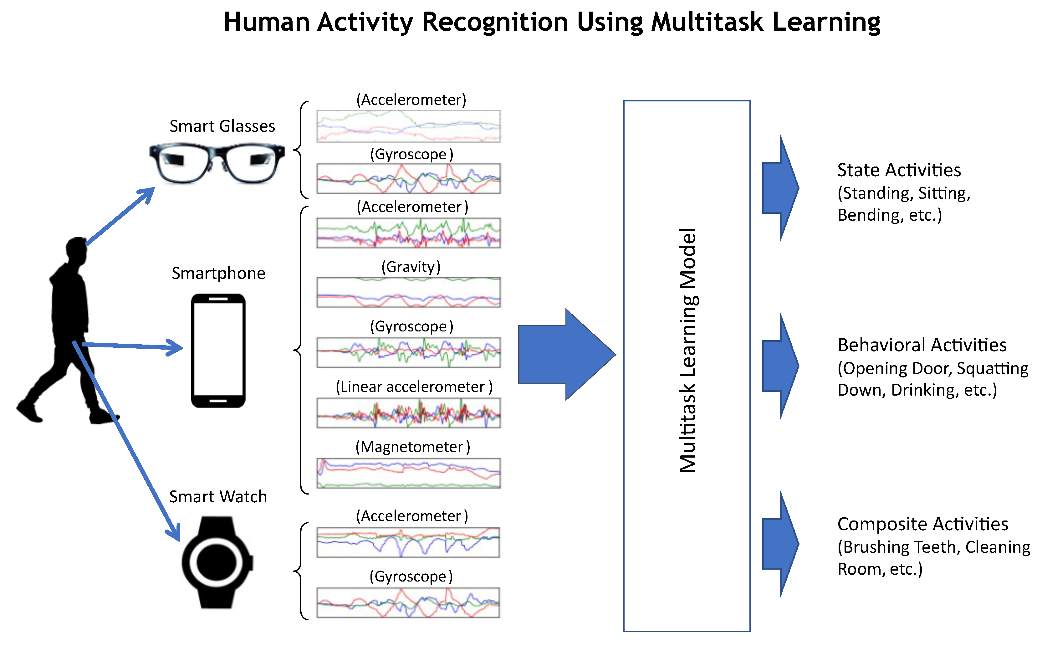
Figure 1.
A multitask learning approach for human activity recognition using multimodal sensor data acquired from wearable devices.
Figure 1.
A multitask learning approach for human activity recognition using multimodal sensor data acquired from wearable devices.
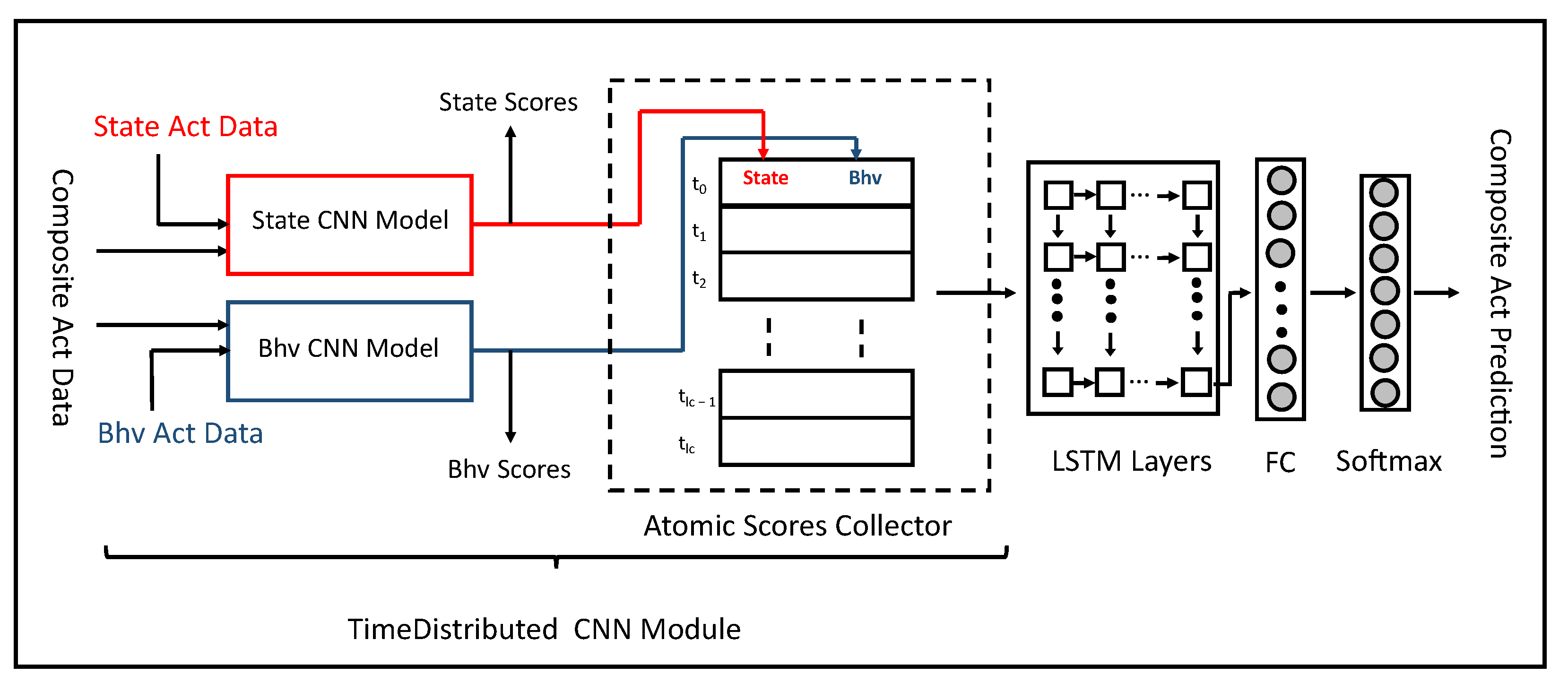
Figure 2.
Overview of the multitask learning architecture to learn state, behavioral, and composite activities together.
Figure 2.
Overview of the multitask learning architecture to learn state, behavioral, and composite activities together.
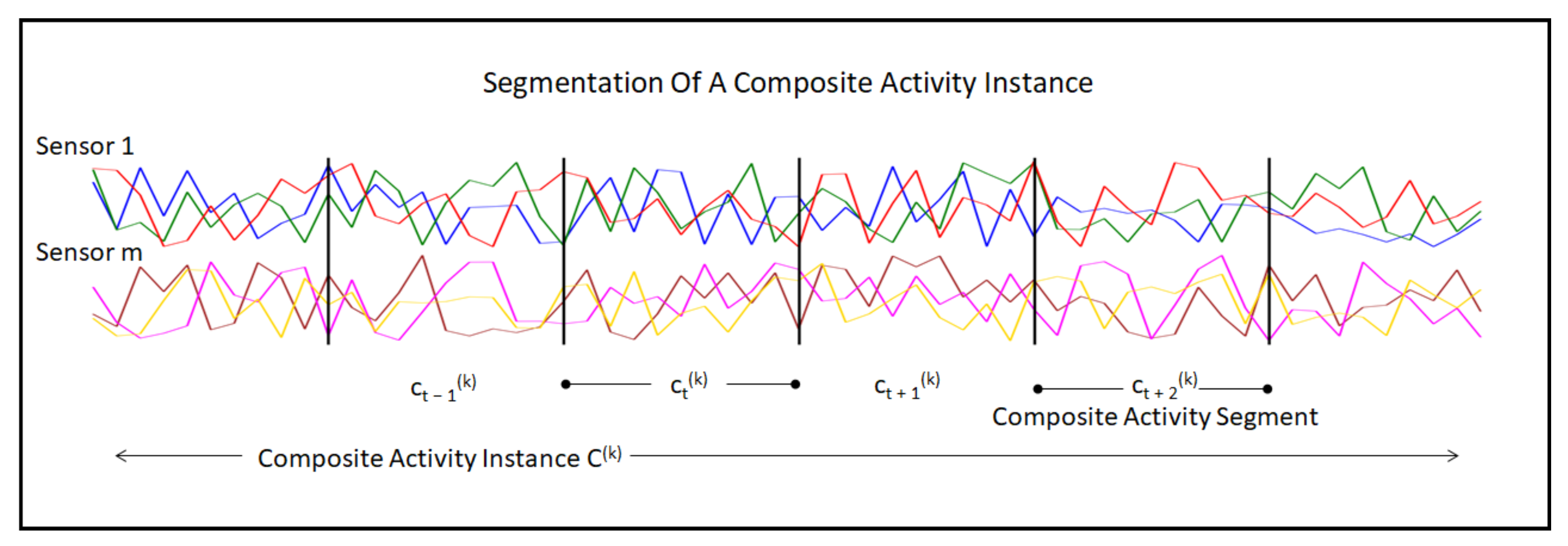
Figure 3.
The figure shows the segmentation of a composite activity instance . Two of the sensor modalities and are shown in the figure. The horizontal axis of the graph represents the time. The equal-size segments of the composite activity instance are represented by .
Figure 3.
The figure shows the segmentation of a composite activity instance . Two of the sensor modalities and are shown in the figure. The horizontal axis of the graph represents the time. The equal-size segments of the composite activity instance are represented by .
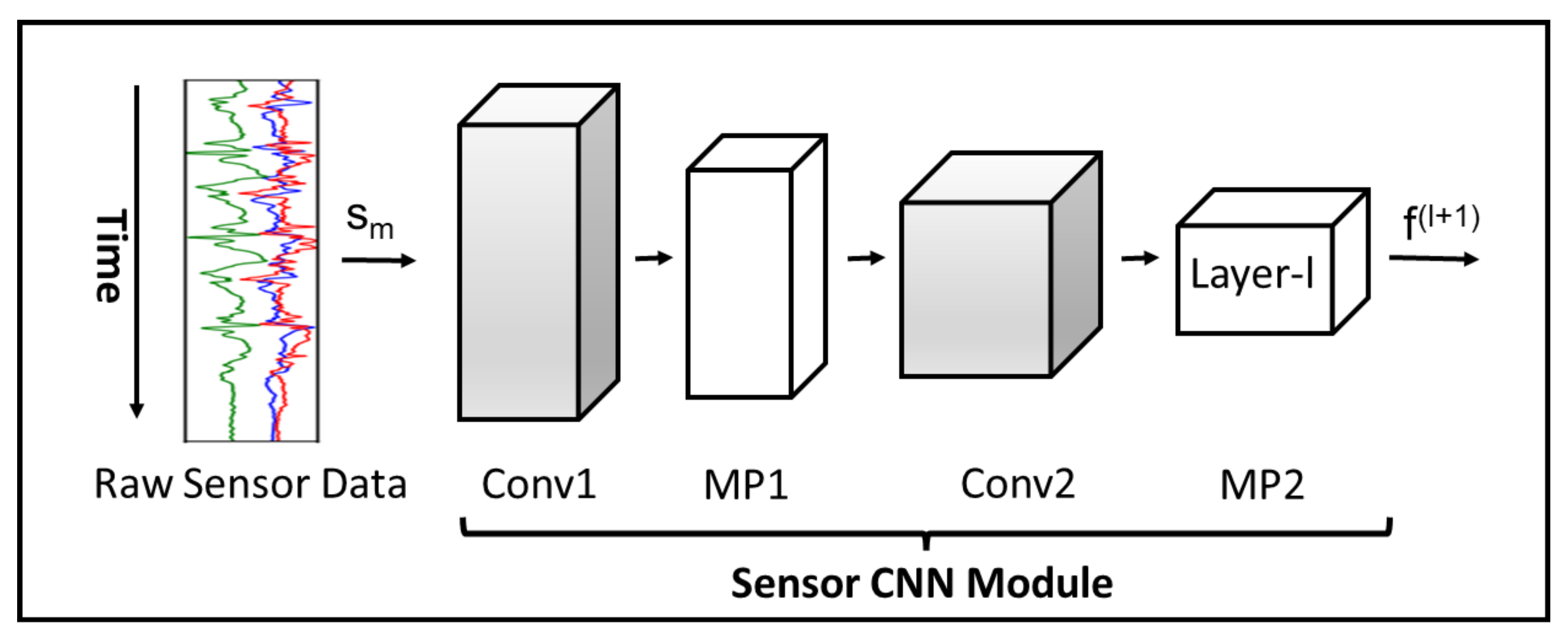
Figure 4.
The sensor module represents a CNN branch of our proposed model. The branch receives raw sensor data of a sensor m for convolutional and max pooling layers. Each layer l receives a feature map as input and produces an output feature map for the next layer.
Figure 4.
The sensor module represents a CNN branch of our proposed model. The branch receives raw sensor data of a sensor m for convolutional and max pooling layers. Each layer l receives a feature map as input and produces an output feature map for the next layer.
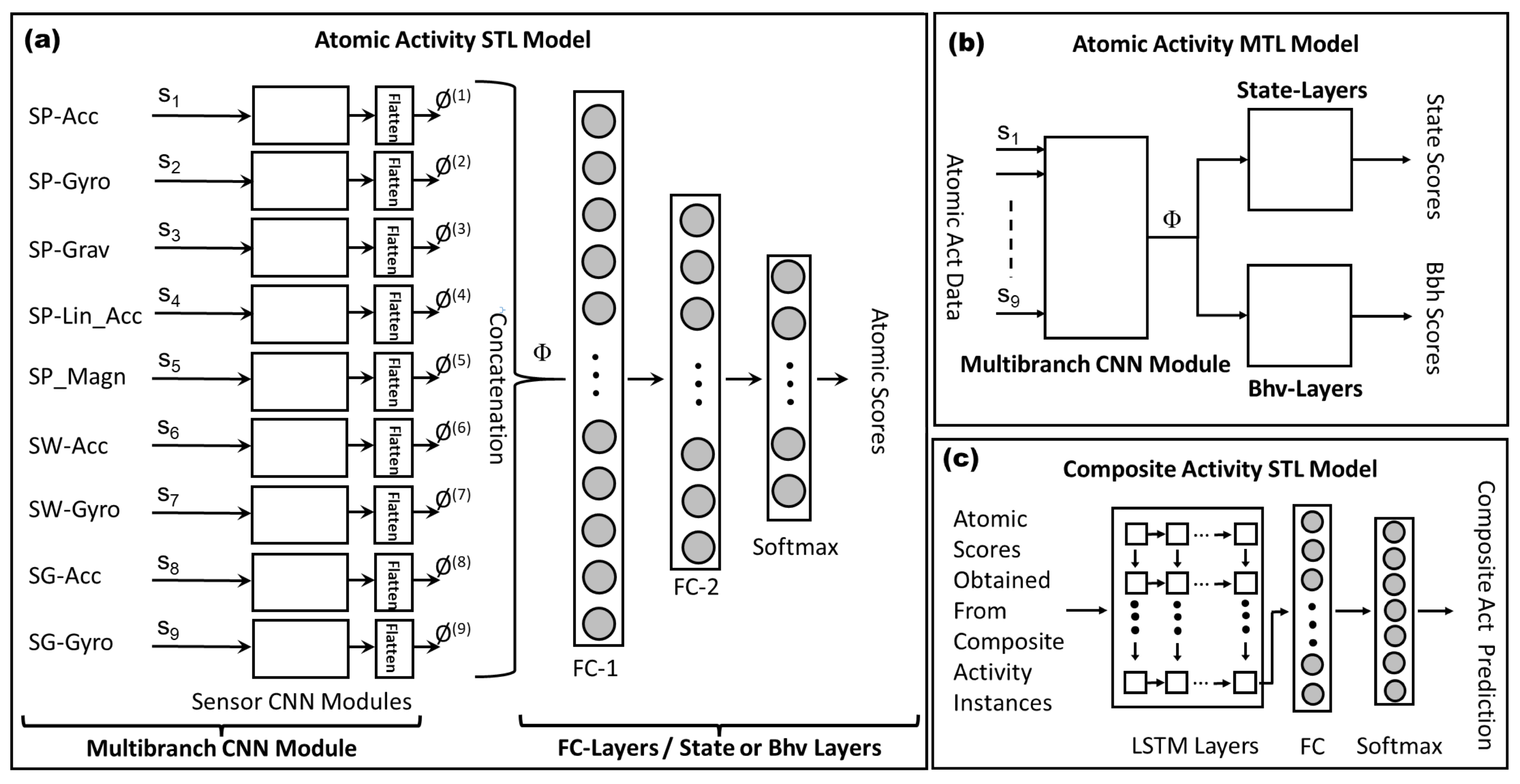
Figure 5.
The figure shows the architectures of three models. The first figure (a) shows the multibranch architecture for the single-task learning (STL) model of atomic activities. State and behavioral activities use this model to generate atomic scores. The second figure (b) is the architecture of the multitask learning (MTL) model for atomic activities. They share the multibranch CNN module; however, they exclusively use their own state and behavioral (bhv) modules. The third figure (c) represents the architecture of the single-task learning model for composite activities. The instances of composite activities are first sent to either STL or MTL atomic models to generate atomic scores. Then, these scores are provided to composite activity STL model for the prediction of the labels.
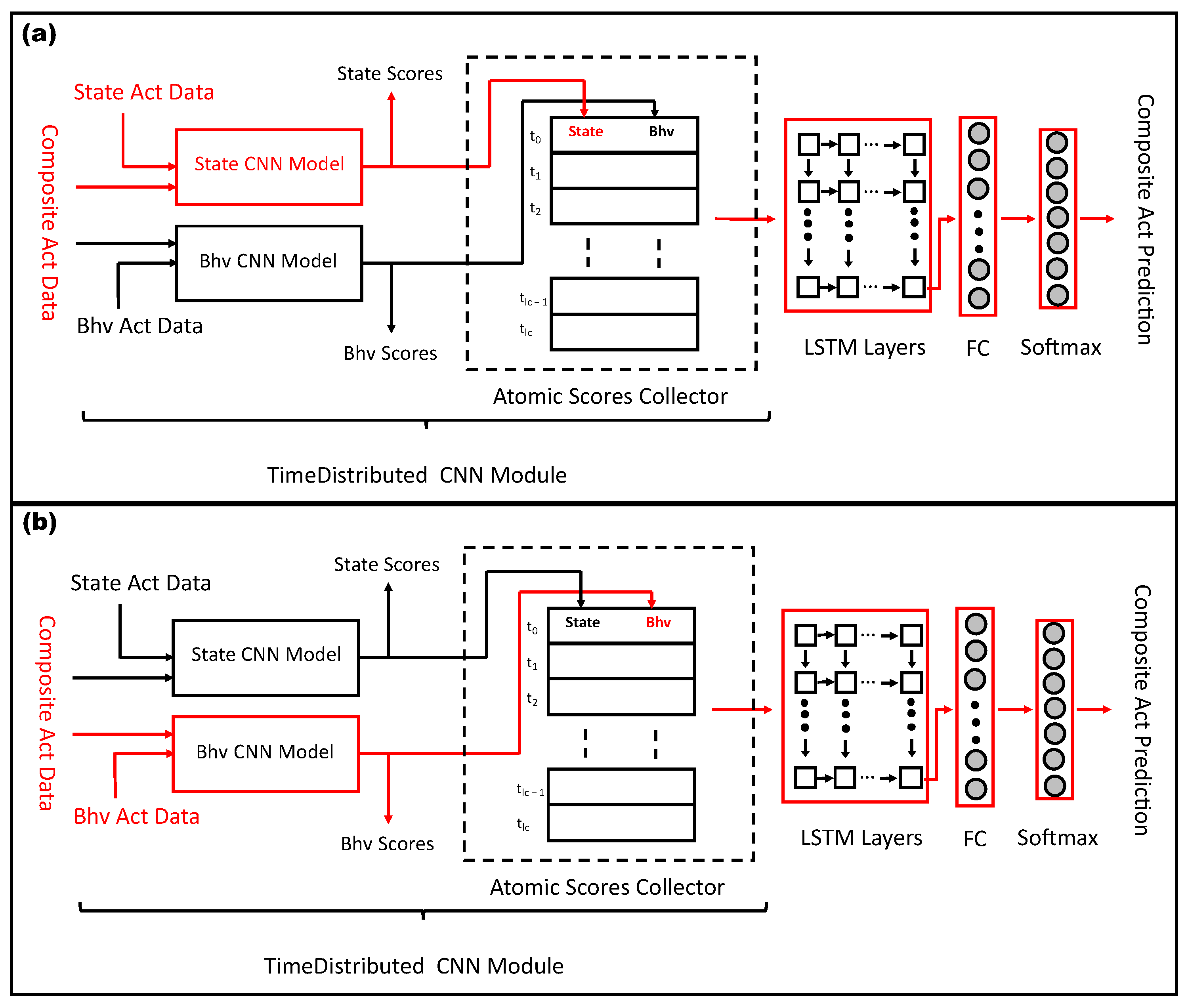
Figure 6.
The architecture of the multitask learning model for atomic and composite activities. The first figure (a) shows the multitask learning of state and composite activities. The second figure (b) shows the multitask learning of behavioral and composite activities.
Figure 6.
The architecture of the multitask learning model for atomic and composite activities. The first figure (a) shows the multitask learning of state and composite activities. The second figure (b) shows the multitask learning of behavioral and composite activities.
Table 3.
Architecture and hyperparameters of the multibranch convolutional module, containing the sequence of layers, the number of convolutional filters and kernel sizes, pooling, and stride sizes used in the model.
Table 3.
Architecture and hyperparameters of the multibranch convolutional module, containing the sequence of layers, the number of convolutional filters and kernel sizes, pooling, and stride sizes used in the model.
| Multibranch CNN Module: Architecture and Hyper Parameters |
|---|
| | |
Sensors
|
|---|
|
Layer
|
Information
|
sp-acc, sp-gyro
|
sp-magn
|
sg-acc
|
|---|
| | |
sp-grav, sp-linAcc
|
(sw-acc, sw-gyro)
|
sg-gyro
|
|---|
| Input | Size | X, 3, 900 | X, 3, 450 | X, 3, 80 |
| Batch normalization | Yes | Yes | Yes |
| Conv 1 | Filters | 16 | 16, (32) | 16 |
| Kern size | 64 | 32 | 8 |
| Activation | reLU | reLU | reLU |
| Max Pool 1 | Pool, Stride | 16, 4 | 16, 2 | 8, 2 |
| Conv 2 | Filters | 32 | 32, (64) | 16 |
| Kern size | 128 | 64 | 8 |
| Activation | reLU | reLU | reLU |
| Max Pool 2 | Pool, Stride | 16, 4 | 16,2 | 8,2 |
| Flattening and Concatenation of All Branches |
Table 4.
Architecture and hyperparameters of state layers, containing the sequence of layers, number of units, activation functions, optimizer, and the loss function used in the model.
Table 4.
Architecture and hyperparameters of state layers, containing the sequence of layers, number of units, activation functions, optimizer, and the loss function used in the model.
| State Layers: Architecture and Hyper Parameters |
|---|
| | |
Sensors
|
|---|
|
Layer
|
Information
|
sp-acc, sp-gyro
|
sp-magn
|
sg-acc
|
|---|
| | |
sp-grav, sp-linAcc
|
(sw-acc, sw-gyro)
|
sg-gyro
|
|---|
| FC 1 | Units State | In: 10,752, Out: 256 | | |
| Activation | | reLU | |
| Dropout | Rate | | 0.3 | |
| FC 2 | Units State | | In: 256, Out: 64 | |
| Activation | | reLU | |
| Dropout | Rate | | 0.3 | |
| Output | Units State | | In: 64, Out: 6 | |
| Activation | | softmax | |
| Optimizer: Adadelta, Learning rate: 0.0001 |
| Loss function: Categorical Cross Entropy |
Table 5.
Architecture and hyperparameters of the behavioral layers, containing the sequence of layers, number of units, activation functions, optimizer, and the loss function used in the model.
Table 5.
Architecture and hyperparameters of the behavioral layers, containing the sequence of layers, number of units, activation functions, optimizer, and the loss function used in the model.
| Behavioral Layers: Architecture and Hyper Parameters |
|---|
| | |
Sensors
|
|---|
|
Layer
|
Information
|
sp-acc, sp-gyro
|
sp-magn
|
sg-acc
|
|---|
| | |
sp-grav, sp-linAcc
|
(sw-acc, sw-gyro)
|
sg-gyro
|
|---|
| FC 1 | Units Bhv | | In: 10,752, Out: 512 | |
| Activation | | reLU | |
| Dropout | Rate | | 0.3 | |
| FC 2 | Units Bhv | | In: 512, Out: 256 | |
| Activation | | reLU | |
| Dropout | Rate | | 0.3 | |
| Output | Units Bhv | | In: 256, Out: 55 | |
| Activation | | softmax | |
| Optimizer: Adadelta, Learning rate: 0.0001 |
| Loss function: Categorical Cross Entropy |
Table 6.
Results (accuracy) obtained from multitask learning models of state and behavioral activities using different weighting strategies. The results of the experiments are obtained by fixing the weight for state activities, to , and computed results using one of the five values for the weight of behavioral activities . The best results were produced using and . Therefore, we used this setting in further experiments of MTL atomic models.
| Comparison of Results with Different Values of Bhv Weights () |
|---|
|
Activity
|
Bhv Weights
|
|---|
| | 1.0 | 0.10 | 0.01 | 0.001 | 0.0001 |
| State | 73.54 | 75.00 | 72.82 | 74.76 | 72.57 |
| Behavioral | 73.55 | 73.34 | 71.63 | 71.09 | 69.14 |
Table 7.
Comparative results (accuracy) obtained from different methods, including multitask learning for atomic and composite activities and the single-task learning of composite activities using different lengths.
Table 7.
Comparative results (accuracy) obtained from different methods, including multitask learning for atomic and composite activities and the single-task learning of composite activities using different lengths.
| Comparison of Results Using Different Lengths of Composite Activity Instances |
|---|
|
Length
|
MTL
|
STL
|
|---|
|
State
|
Bhv
|
Composite
|
Holdout
|
Train-Test
|
|---|
| 18 s | 64.56 | 30.61 | 80.63 | 39.90 | 77.92 |
| 45 s | 44.66 | 32.35 | 81.85 | 42.38 | 81.47 |
| 90 s | 69.18 | 67.01 | 82.83 | 46.31 | 83.21 |
| Actual | 72.82 | 71.63 | 92.87 | 54.87 | 90.89 |
Table 8.
Architecture and hyperparameters of the LSTM module, containing the sequence of layers, number of units, activation functions, optimizer, and the loss function used in the model.
Table 8.
Architecture and hyperparameters of the LSTM module, containing the sequence of layers, number of units, activation functions, optimizer, and the loss function used in the model.
| LSTM Module: Architecture and Hyper Parameters |
|---|
|
Layer
|
Information
|
|---|
| Timedistributed- | Input: Sensors’ data of all () segments of an instance |
| State model | Output: An array of score-vectors; each vector contains 6 state scores |
| Timedistributed- | Input: Sensors’ data of all () segments of an instance |
| Behavioral model | Output: An array of score-vectors; each vector contains 55 behavioral scores |
| Concatenation of state and behavioral score-vectors |
| LSTM layers | Input size: 61 |
| Hidden units: 128 |
| Num of layers: 2 |
| Output | Input size: 128, Output size: 7 |
| Optimizer: Adadelta, Learning rate: 0.00001 |
| Loss function: Categorical Cross-Entropy |
Table 9.
Comparison of results of state and behavioral activities obtained from different methods. The results have been compared using three methods, “codebook and SVM approach”, “multibranch CNN using single-task learning(STL)”, and “multibranch CNN architecture using multitask learning(MTL)”, as explained in the methodology section. The atomic and composite models were trained and evaluated using train–test data settings.
| Recognition of State, Behavioral & Composite Activities (Train-Test) |
|---|
|
Method
|
State
|
Behavioral
|
Composite
|
|---|
|
Atomic
|
Composite
|
Acc
|
AF1
|
Acc
|
AF1
|
Acc
|
AF1
|
|---|
| Codebook | RP | 88.58 | 88.22 | 68.23 | 67.92 | 81.49 | 80.92 |
| Codebook | RP + MP + AP | 88.49 | 87.98 |
| CNN | RP | 92.41 | 92.32 | 71.83 | 71.68 | 82.89 | 82.57 |
| STL Multibranch-CNN | STL Td LSTM | 93.69 | 92.71 | 73.66 | 73.22 | 91.31 | 90.89 |
| MTL Multibranch-CNN | STL Td LSTM | 77.43 | 77.48 | 72.03 | 71.30 | 91.98 | 91.79 |
| MTL_Atomic_Composite | 74.27 | 73.25 | 72.19 | 71.66 | 92.87 | 92.32 |
| MTL_(State-Comp, Bhv-Comp) | 95.15 | 95.07 | 73.93 | 73.38 | 93.99 | 93.76 |
Table 10.
Comparison of results of state and behavioral activities obtained from different methods. The results have been compared using three methods: codebook and SVM approach, multibranch CNN using single-task learning (STL), and multibranch CNN architecture using multitask learning (MTL), as explained in the methodology section. The atomic models were trained and evaluated using train–test settings, whereas composite activity models were trained and evaluated using train–test data settings.
| Recognition of State, Behavioral and Composite Activities (Holdout) |
|---|
|
Method
|
State
|
Behavioral
|
Composite
|
|---|
|
Atomic
|
Composite
|
Acc
|
AF1
|
Acc
|
AF1
|
Acc
|
AF1
|
|---|
| Codebook | RP | 88.58 | 88.22 | 68.23 | 67.92 | 61.48 | 60.91 |
| Codebook | RP + MP + AP | 63.64 | 63.65 |
| CNN | RP | 92.41 | 92.32 | 71.83 | 71.68 | 54.98 | 54.31 |
| STL Multibranch-CNN | STL Td LSTM | 93.69 | 92.71 | 73.66 | 73.22 | 59.62 | 53.61 |
| MTL Multibranch-CNN | STL Td LSTM | 77.43 | 77.48 | 72.03 | 71.30 | 55.11 | 51.76 |
| MTL_Atomic_Composite | 76.94 | 76.33 | 71.63 | 71.42 | 76.01 | 75.80 |
| MTL_(State-Comp, Bhv-Comp) | 94.90 | 94.85 | 73.48 | 73.10 | 70.55 | 69.01 |
Table 11.
Comparison of results of state and behavioral activities obtained from different methods. The results have been compared using three methods: codebook and SVM approach, multibranch CNN using single-task learning(STL), and multibranch CNN architecture using multitask learning(MTL) as explained in the methodology section. The atomic models were trained and evaluated using train-test settings whereas composite activity models were trained and evaluated using LOSO-CV data settings.
| Recognition of State, Behavioral & Composite Activities (LOSO-CV) |
|---|
|
Method
|
State
|
Behavioral
|
Composite
|
|---|
|
Atomic
|
Composite
|
Acc
|
AF1
|
Acc
|
AF1
|
Acc
|
AF1
|
|---|
| Codebook | RP | 88.58 | 88.22 | 68.23 | 67.92 | 64.58 | 62.23 |
| Codebook | (RP + MP + AP) | 88.58 | 88.22 | 68.23 | 67.92 | 68.65 | 64.39 |
| CNN | RP | 92.41 | 92.32 | 71.83 | 71.68 | 56.80 | 52.85 |
| STL Multibranch-CNN | STL Td LSTM | 93.69 | 92.71 | 73.66 | 73.22 | 77.37 | 76.60 |
| MTL Multibranch-CNN | STL Td LSTM | 77.43 | 77.48 | 72.03 | 71.30 | 72.22 | 70.11 |
| MTL_Atomic_Composite | 75.00 | 74.96 | 72.18 | 71.66 | 82.31 | 80.67 |
| MTL_(State-Comp, Bhv-Comp) | 93.77 | 93.07 | 73.73 | 73.38 | 81.28 | 80.72 |
Table 12.
Comparison of results obtained from multitask learning method. The two-branch MTL model was jointly trained for state and composite activities in one branch and behavioral and composite activities in the second branch. The results were obtained in the LOSO-CV settings of the composite activity dataset.
| LOSO-CV: Multitask Learning for State, Bhv and Composite Activities |
|---|
|
Pass
|
State
|
Behavioral
|
Composite
|
|---|
| Pass-1 | 93.45 | 73.82 | 90.00 |
| Pass-2 | 95.39 | 73.93 | 71.93 |
| Pass-3 | 92.72 | 73.56 | 77.63 |
| Pass-4 | 93.20 | 74.44 | 81.51 |
| Pass-5 | 94.16 | 72.79 | 90.71 |
| Pass-6 | 93.69 | 73.85 | 75.91 |
| Average | 93.77 | 73.73 | 81.28 |
Table 13.
Performance comparison of multitask learning for two types of activities.
Table 13.
Performance comparison of multitask learning for two types of activities.
| Activity | State | Behavioral | Composite |
|---|
| State + Behavioral | 77.43 | 72.03 | - |
| State + Composite | 95.17 | - | 92.43 |
| Behavioral + Composite | - | 73.92 | 93.32 |
Table 14.
Confusion matrix of state activities obtained from the MTL model of state and behavioral activities. The values in the circles show that most of the misclassification occurred in sitting and standing state activities.
Table 14.
Confusion matrix of state activities obtained from the MTL model of state and behavioral activities. The values in the circles show that most of the misclassification occurred in sitting and standing state activities.
| State Activities—Confusion Matrix—MTL State and Behavioral |
|---|
|
Activities
|
Bending
|
Lying
|
Sitting
|
Squatting
|
Standing
|
Walking
|
|---|
| Bending | 69 | 0 | 0 | 0 | 0 | 0 |
| Lying | 6 | 63 | 0 | 0 | 0 | 0 |
| Sitting | | 2 | 19 | 3 | 0 | 0 |
| Squatting | 17 | 0 | 2 | 48 | 0 | 0 |
| Standing | | 0 | 0 | 0 | 27 | 0 |
| Walking | 5 | 0 | 0 | 0 | 0 | 65 |

 ,
, 


