
Deep Learning Approach for the Localization and Analysis of Surface Plasmon Scattering

Abstract
:1. Introduction
2. Materials and Methods
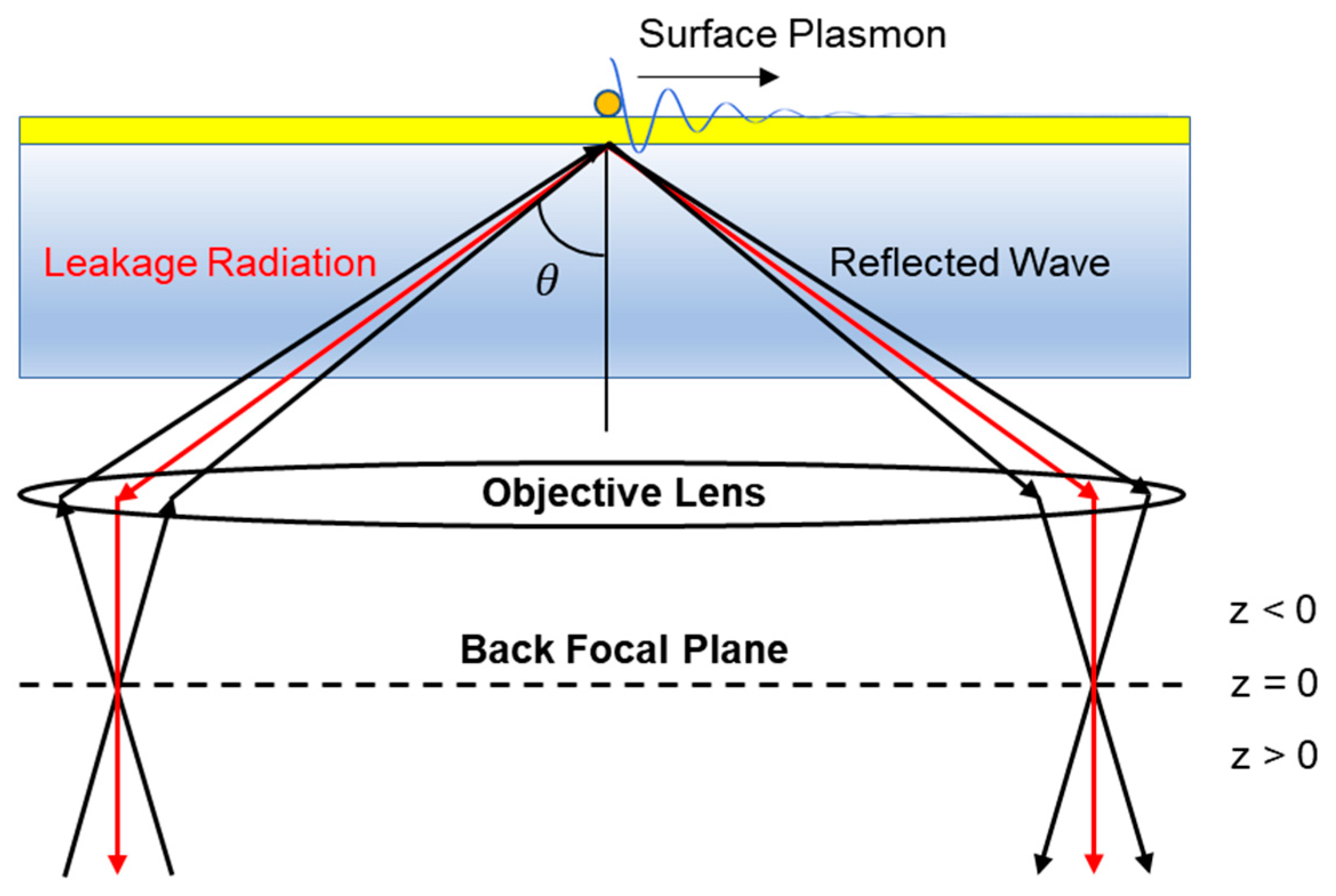
2.1. Scattering Simulation Model
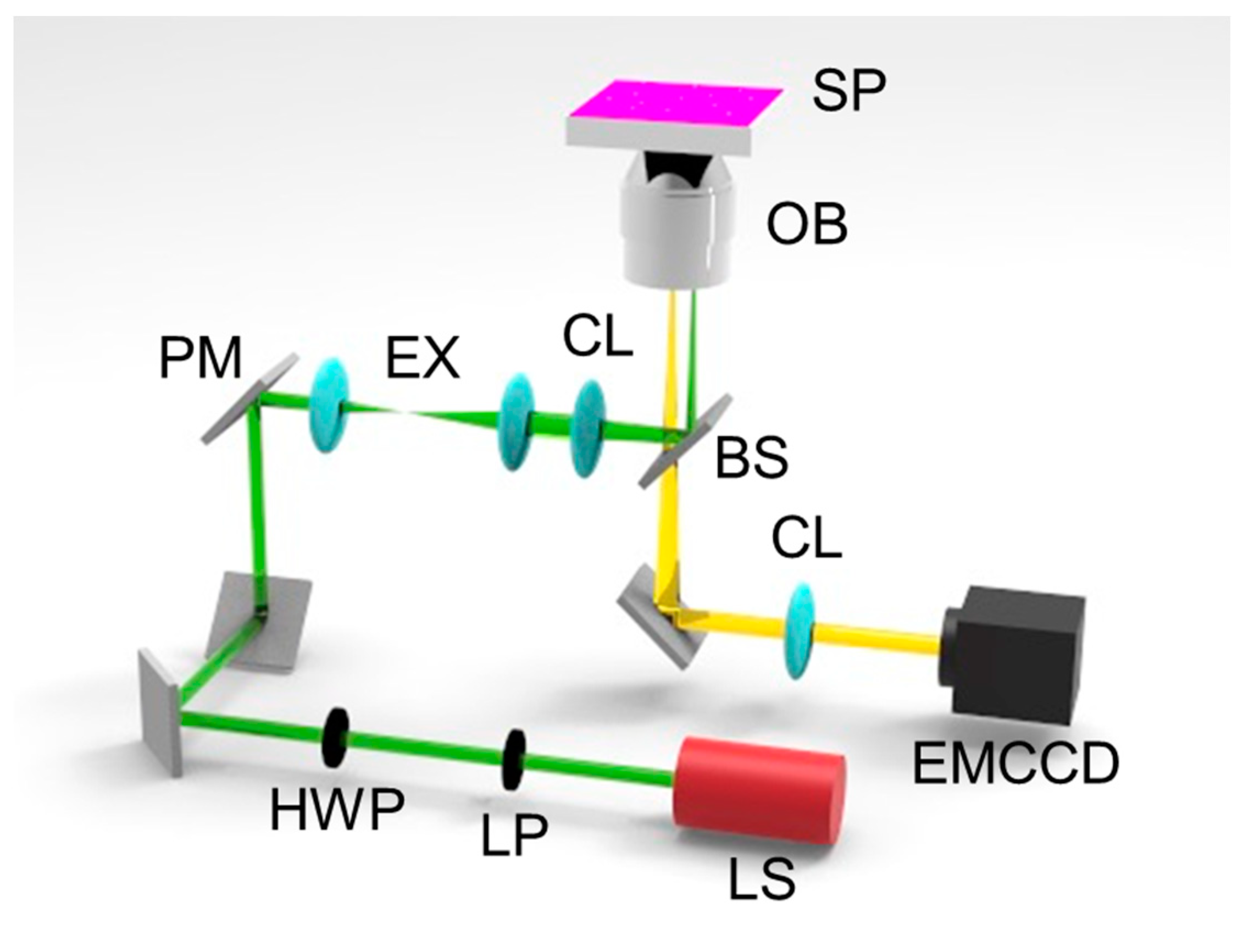
2.2. Optical Configuration
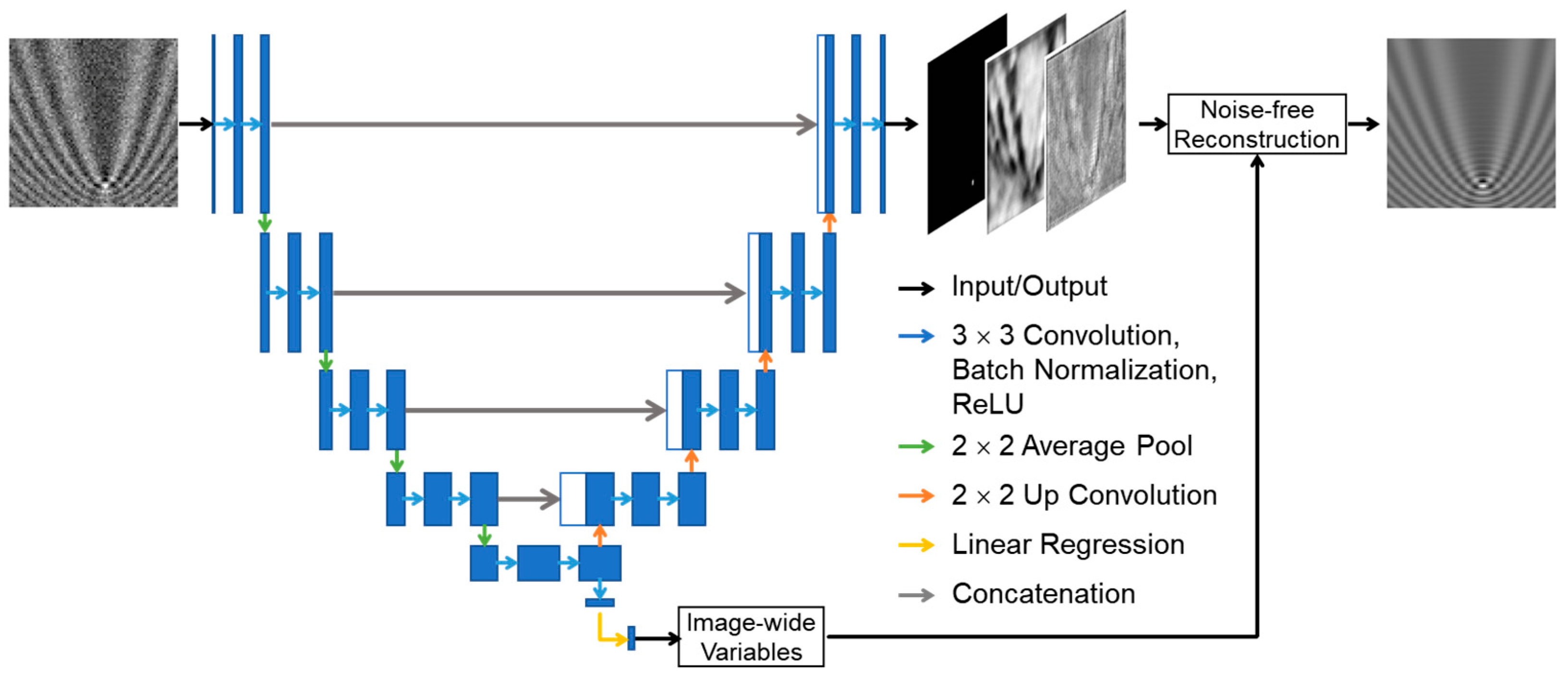
2.3. Modified Y-Net
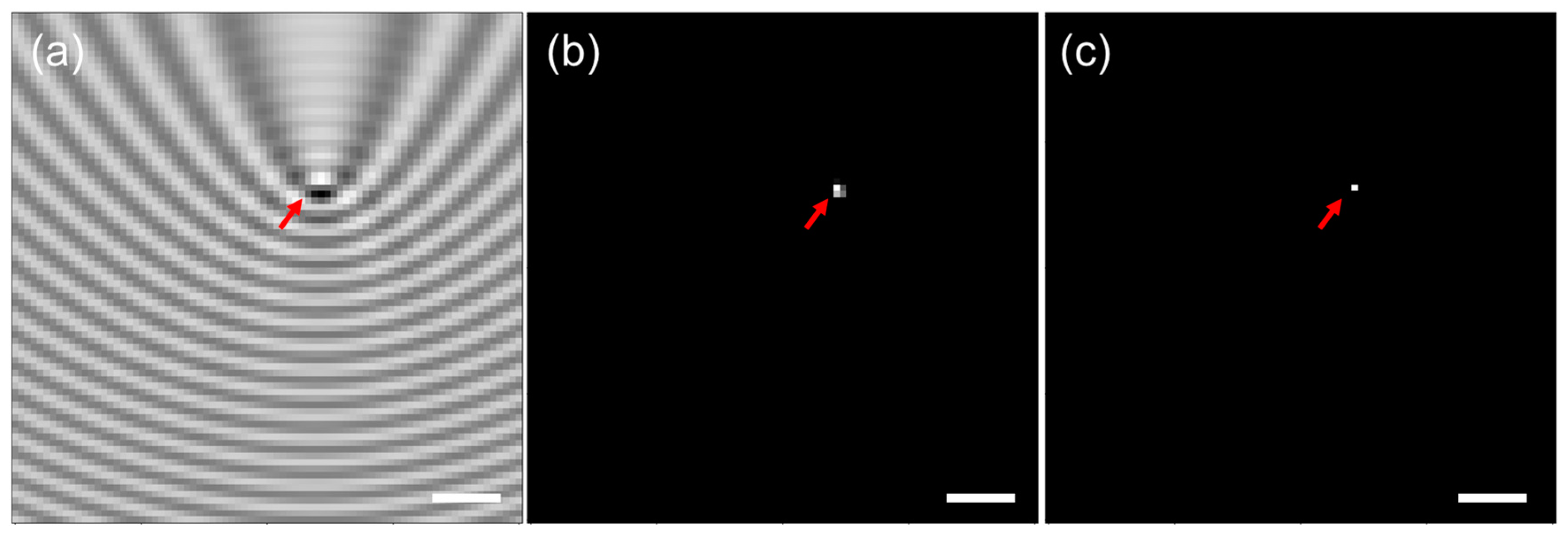
3. Results
4. Discussion
5. Conclusions
Supplementary Materials
Author Contributions
Funding
Institutional Review Board Statement
Informed Consent Statement
Data Availability Statement
Conflicts of Interest
References
- Leighton, R.E.; Alperstein, A.M.; Frontiera, R.R. Label-Free Super-Resolution Imaging Techniques. Annu. Rev. Anal. Chem. 2022, 15, 37–55. [Google Scholar] [CrossRef] [PubMed]
- Son, T.; Lee, C.; Seo, J.; Choi, I.-H.; Kim, D. Surface Plasmon Microscopy by Spatial Light Switching for Label-free Imaging with Enhanced Resolution. Opt. Lett. 2018, 43, 959–962. [Google Scholar] [CrossRef] [PubMed]
- Zeng, S.; Baillargeat, D.; Ho, H.-P.; Yong, K.-T. Nanomaterials Enhanced Surface Plasmon Resonance for Biological and Chemical Sensing Applications. Chem. Soc. Rev. 2014, 43, 3426. [Google Scholar] [CrossRef] [PubMed]
- Marx, V. It’s Free Imaging—Label-Free, That Is. Nat. Methods 2019, 16, 1209–1212. [Google Scholar] [CrossRef]
- Freudiger, C.W.; Min, W.; Saar, B.G.; Lu, S.; Holtom, G.R.; He, C.; Tsai, J.C.; Kang, J.X.; Xie, X.S. Label-Free Biomedical Imaging with High Sensitivity by Stimulated Raman Scattering Microscopy. Science 2008, 322, 1857–1861. [Google Scholar] [CrossRef]
- Halpern, A.R.; Chen, Y.; Corn, R.M.; Kim, D. Surface Plasmon Resonance Phase Imaging Measurements of Patterned Monolayers and DNA Adsorption onto Microarrays. Anal. Chem. 2011, 83, 2801–2806. [Google Scholar] [CrossRef]
- Huang, B.; Yu, F.; Zare, R.N. Surface Plasmon Resonance Imaging Using a High Numerical Aperture Microscope Objective. Anal. Chem. 2007, 79, 2979–2983. [Google Scholar] [CrossRef]
- Jiang, Y.; Wang, W. Point Spread Function of Objective-Based Surface Plasmon Resonance Microscopy. Anal. Chem. 2018, 90, 9650–9656. [Google Scholar] [CrossRef]
- Son, T.; Kim, D. Theoretical Approach to Surface Plasmon Scattering Microscopy for Single Nanoparticle Detection in Near Infrared Region. In Proceedings of the Plasmonics in Biology and Medicine XII. Vol. 9340. (SPIE 2015), San Francisco, CA, USA, 11 March 2015; pp. 113–118. [Google Scholar]
- Nizamov, S.; Scherbahn, V.; Mirsky, V.M. Detection and Quantification of Single Engineered Nanoparticles in Complex Samples Using Template Matching in Wide-Field Surface Plasmon Microscopy. Anal. Chem. 2016, 88, 10206–10214. [Google Scholar] [CrossRef]
- Giebel, K.-F.; Bechinger, C.; Herminghaus, S.; Riedel, M.; Leiderer, P.; Weiland, U.; Bastmeyer, M. Imaging of Cell/Substrate Contacts of Living Cells with Surface Plasmon Resonance Microscopy. Biophys. J. 1999, 76, 509–516. [Google Scholar] [CrossRef]
- Halpern, A.R.; Wood, J.B.; Wang, Y.; Corn, R.M. Single-Nanoparticle Near-Infrared Surface Plasmon Resonance Microscopy for Real-Time Measurements of DNA Hybridization Adsorption. ACS Nano 2014, 8, 1022–1030. [Google Scholar] [CrossRef] [PubMed]
- Zhou, X.; Yang, Y.; Wang, S.; Liu, X. Surface Plasmon Resonance Microscopy: From Single-Molecule Sensing to Single-Cell Imaging. Angew. Chem. Int. Ed. 2020, 59, 1776–1785. [Google Scholar] [CrossRef] [PubMed]
- Son, T.; Seo, J.; Choi, I.-H.; Kim, D. Label-Free Quantification of Cell-to-Substrate Separation by Surface Plasmon Resonance Microscopy. Opt. Commun. 2018, 422, 64–68. [Google Scholar] [CrossRef]
- Nizamov, S.; Scherbahn, V.; Mirsky, V.M. Ionic Referencing in Surface Plasmon Microscopy: Visualization of the Difference in Surface Properties of Patterned Monomolecular Layers. Anal. Chem. 2017, 89, 3873–3878. [Google Scholar] [CrossRef] [PubMed]
- Kim, D.J.; Kim, D. Subwavelength Grating-Based Nanoplasmonic Modulation for Surface Plasmon Resonance Imaging with Enhanced Resolution. J. Opt. Soc. Am. B 2010, 27, 1252–1259. [Google Scholar] [CrossRef]
- Wang, S.; Shan, X.; Patel, U.; Huang, X.; Lu, J.; Li, J.; Tao, N. Label-Free Imaging, Detection, and Mass Measurement of Single Viruses by Surface Plasmon Resonance. Proc. Natl. Acad. Sci. USA 2010, 107, 16028–16032. [Google Scholar] [CrossRef]
- Wang, W.; Wang, S.; Liu, Q.; Wu, J.; Tao, N. Mapping Single-Cell–Substrate Interactions by Surface Plasmon Resonance Microscopy. Langmuir 2012, 28, 13373–13379. [Google Scholar] [CrossRef]
- Yang, Y.; Shen, G.; Wang, H.; Li, H.; Zhang, T.; Tao, N.; Ding, X.; Yu, H. Interferometric Plasmonic Imaging and Detection of Single Exosomes. Proc. Natl. Acad. Sci. USA 2018, 115, 10275–10280. [Google Scholar] [CrossRef]
- Krizhevsky, A.; Sutskever, I.; Hinton, G.E. ImageNet Classification with Deep Convolutional Neural Networks. Commun. ACM 2017, 60, 84–90. [Google Scholar] [CrossRef]
- Alipanahi, B.; Delong, A.; Weirauch, M.T.; Frey, B.J. Predicting the Sequence Specificities of DNA- and RNA-Binding Proteins by Deep Learning. Nat. Biotechnol. 2015, 33, 831–838. [Google Scholar] [CrossRef]
- Nguyen, T.; Bui, V.; Lam, V.; Raub, C.B.; Chang, L.-C.; Nehmetallah, G. Automatic Phase Aberration Compensation for Digital Holographic Microscopy Based on Deep Learning Background Detection. Opt. Express 2017, 25, 15043. [Google Scholar] [CrossRef] [PubMed]
- Ballard, Z.S.; Shir, D.; Bhardwaj, A.; Bazargan, S.; Sathianathan, S.; Ozcan, A. Computational Sensing Using Low-Cost and Mobile Plasmonic Readers Designed by Machine Learning. ACS Nano 2017, 11, 2266–2274. [Google Scholar] [CrossRef] [PubMed]
- Kamilov, U.S.; Papadopoulos, I.N.; Shoreh, M.H.; Goy, A.; Vonesch, C.; Unser, M.; Psaltis, D. Learning Approach to Optical Tomography. Optica 2015, 2, 517. [Google Scholar] [CrossRef]
- Satat, G.; Tancik, M.; Gupta, O.; Heshmat, B.; Raskar, R. Object Classification through Scattering Media with Deep Learning on Time Resolved Measurement. Opt. Express 2017, 25, 17466. [Google Scholar] [CrossRef]
- Horisaki, R.; Takagi, R.; Tanida, J. Learning-Based Imaging through Scattering Media. Opt. Express 2016, 24, 13738. [Google Scholar] [CrossRef]
- Esteva, A.; Kuprel, B.; Novoa, R.A.; Ko, J.; Swetter, S.M.; Blau, H.M.; Thrun, S. Dermatologist-Level Classification of Skin Cancer with Deep Neural Networks. Nature 2017, 542, 115–118. [Google Scholar] [CrossRef]
- Chen, C.L.; Mahjoubfar, A.; Tai, L.-C.; Blaby, I.K.; Huang, A.; Niazi, K.R.; Jalali, B. Deep Learning in Label-Free Cell Classification. Sci. Rep. 2016, 6, 21471. [Google Scholar] [CrossRef]
- Moon, G.; Choi, J.; Lee, C.; Oh, Y.; Kim, K.H.; Kim, D. Machine Learning-Based Design of Meta-Plasmonic Biosensors with Negative Index Metamaterials. Biosens. Bioelectron. 2020, 164C, 112335. [Google Scholar] [CrossRef]
- Kim, J.; Lee, H.; Im, S.; Lee, S.A.; Kim, D.; Toh, K.-A. Machine Learning-Based Leaky Momentum Prediction of Plasmonic Random Nanosubstrate. Opt. Express 2021, 29, 30625–30636. [Google Scholar] [CrossRef]
- Moon, G.; Lee, J.; Lee, H.; Yoo, H.; Ko, K.; Im, S.; Kim, D. Machine Learning and Its Applications for Plasmonics in Biology. Cell Rep. Phys. Sci. 2022, 3, 101042. [Google Scholar] [CrossRef]
- Moon, G.; Son, T.; Lee, H.; Kim, D. Deep Learning Approach for Enhanced Detection of Surface Plasmon Scattering. Anal. Chem. 2019, 91, 9538–9545. [Google Scholar] [CrossRef] [PubMed]
- Yang, Y.; Zhai, C.; Zeng, Q.; Khan, A.L.; Yu, H. Multifunctional Detection of Extracellular Vesicles with Surface Plasmon Resonance Microscopy. Anal. Chem. 2020, 92, 4884–4890. [Google Scholar] [CrossRef] [PubMed]
- Thadson, K.; Visitsattapongse, S.; Pechprasarn, S. Deep Learning-Based Single-Shot Phase Retrieval Algorithm for Surface Plasmon Resonance Microscope Based Refractive Index Sensing Application. Sci. Rep. 2021, 11, 16289. [Google Scholar] [CrossRef] [PubMed]
- Yu, H.; Shan, X.; Wang, S.; Chen, H.; Tao, N. Molecular Scale Origin of Surface Plasmon Resonance Biosensors. Anal. Chem. 2014, 86, 8992–8997. [Google Scholar] [CrossRef] [PubMed]
- Kim, K.; Yoon, S.J.; Kim, K. Nanowire-Based Enhancement of Localized Surface Plasmon Resonance for Highly Sensitive Detection: A Theoretical Study. Opt. Express 2006, 14, 12419–12431. [Google Scholar] [CrossRef]
- Kim, D. Effect of Resonant Localized Plasmon Coupling on the Sensitivity Enhancement of Nanowire-Based Surface Plasmon Resonance Biosensors. J. Opt. Soc. Am. A 2006, 23, 2307–2314. [Google Scholar] [CrossRef]
- Kim, K.; Yajima, J.; Oh, Y.; Lee, W.; Oowada, S.; Nishizaka, T.; Kim, D. Nanoscale Localization Sampling Based on Nanoantenna Arrays for Super-resolution Imaging of Fluorescent Monomers on Sliding Microtubules. Small 2012, 8, 892–900. [Google Scholar] [CrossRef]
- Oh, Y.; Lee, W.; Kim, Y.; Kim, D. Self-Aligned Colocalization of 3D Plasmonic Nanogap Arrays for Ultra-Sensitive Surface Plasmon Resonance Detection. Biosens. Bioelectron. 2014, 51, 401–407. [Google Scholar] [CrossRef]
- Lee, W.; Kinosita, Y.; Oh, Y.; Mikami, N.; Yang, H.; Miyata, M.; Nishizaka, T.; Kim, D. Three-Dimensional Superlocalization Imaging of Gliding Mycoplasma mobile by Extraordinary Light Transmission through Arrayed Nanoholes. ACS Nano 2015, 9, 10896–10908. [Google Scholar] [CrossRef]
- Yang, Y.; Zhai, C.; Zeng, Q.; Khan, A.L.; Yu, H. Quantitative Amplitude and Phase Imaging with Interferometric Plasmonic Microscopy. ACS Nano 2019, 13, 13595–13601. [Google Scholar] [CrossRef]
- Yu, H.; Shan, X.; Wang, S.; Chen, H.; Tao, N. Plasmonic Imaging and Detection of Single DNA Molecules. ACS Nano 2014, 8, 3427–3433. [Google Scholar] [CrossRef] [PubMed]
- Ronneberger, O.; Fischer, P.; Brox, T. U-Net: Convolutional Networks for Biomedical Image Segmentation. In Medical Image Computing and Computer-Assisted Intervention—MICCAI 2015, Proceedings of the 18th International Conference, Munich, Germany, 5–9 October 2015; Navab, N., Hornegger, J., Wells, W.M., Frangi, A.F., Eds.; Lecture Notes in Computer Science; Springer International Publishing: Cham, Switzerland, 2015; Volume 9351, pp. 234–241. ISBN 978-3-319-24573-7. [Google Scholar]
- Mehta, S.; Mercan, E.; Bartlett, J.; Weaver, D.; Elmore, J.G.; Shapiro, L. Y-Net: Joint Segmentation and Classification for Diagnosis of Breast Biopsy Images. In Medical Image Computing and Computer Assisted Intervention—MICCAI 2018, Proceedings of the 21st International Conference, Granada, Spain, 16–20 September 2018; Frangi, A.F., Schnabel, J.A., Davatzikos, C., Alberola-López, C., Fichtinger, G., Eds.; Lecture Notes in Computer Science; Springer International Publishing: Cham, Switzerland, 2018; Volume 11071, pp. 893–901. ISBN 978-3-030-00933-5. [Google Scholar]
- Buslaev, A.; Iglovikov, V.I.; Khvedchenya, E.; Parinov, A.; Druzhinin, M.; Kalinin, A.A. Albumentations: Fast and Flexible Image Augmentations. Information 2020, 11, 125. [Google Scholar] [CrossRef]


Disclaimer/Publisher’s Note: The statements, opinions and data contained in all publications are solely those of the individual author(s) and contributor(s) and not of MDPI and/or the editor(s). MDPI and/or the editor(s) disclaim responsibility for any injury to people or property resulting from any ideas, methods, instructions or products referred to in the content. |
© 2023 by the authors. Licensee MDPI, Basel, Switzerland. This article is an open access article distributed under the terms and conditions of the Creative Commons Attribution (CC BY) license (https://creativecommons.org/licenses/by/4.0/).
Share and Cite
Lee, J.; Moon, G.; Ka, S.; Toh, K.-A.; Kim, D. Deep Learning Approach for the Localization and Analysis of Surface Plasmon Scattering. Sensors 2023, 23, 8100. https://doi.org/10.3390/s23198100
Lee J, Moon G, Ka S, Toh K-A, Kim D. Deep Learning Approach for the Localization and Analysis of Surface Plasmon Scattering. Sensors. 2023; 23(19):8100. https://doi.org/10.3390/s23198100
Chicago/Turabian StyleLee, Jongha, Gwiyeong Moon, Sukhyeon Ka, Kar-Ann Toh, and Donghyun Kim. 2023. "Deep Learning Approach for the Localization and Analysis of Surface Plasmon Scattering" Sensors 23, no. 19: 8100. https://doi.org/10.3390/s23198100