
Experimental Investigations of Distributed Fiber Optic Sensors for Water Pipeline Monitoring
 , ,
, ,  , and
, and
Abstract
:1. Introduction
2. Materials and Method
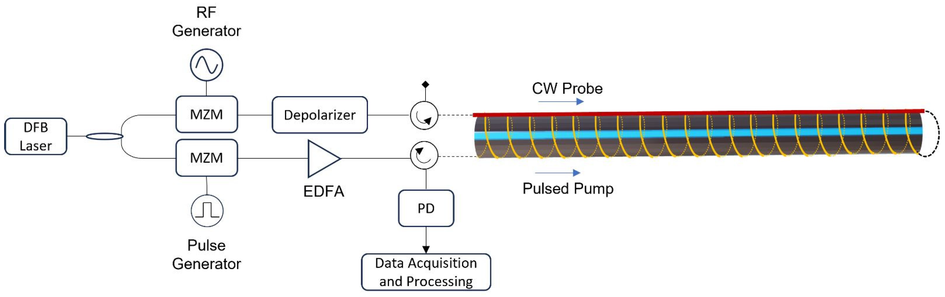
2.1. Sensor Technology and Layout
2.2. Phase I: Assessment of the Sensitivity of the Sensor Layout
2.3. Phase II: Detection of Water Leakage
3. Results
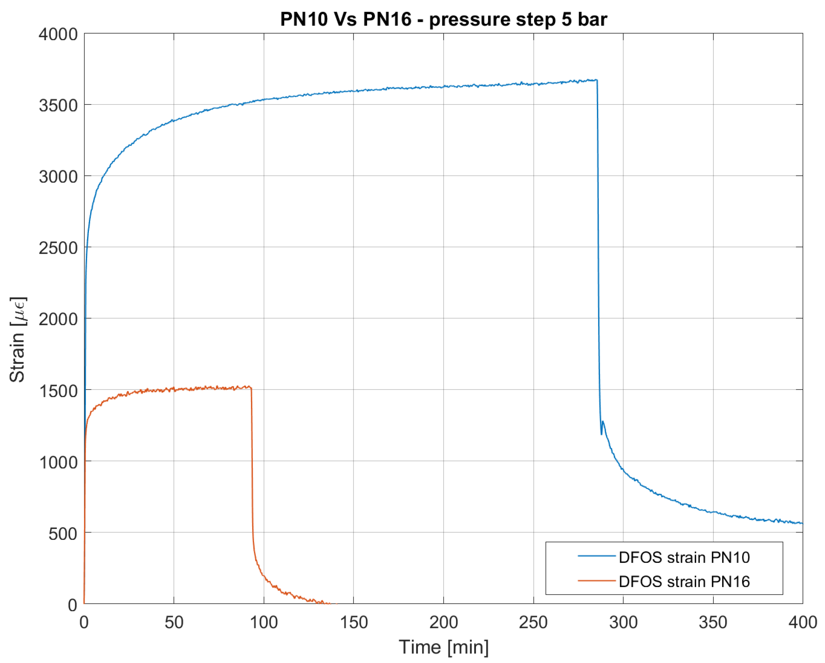
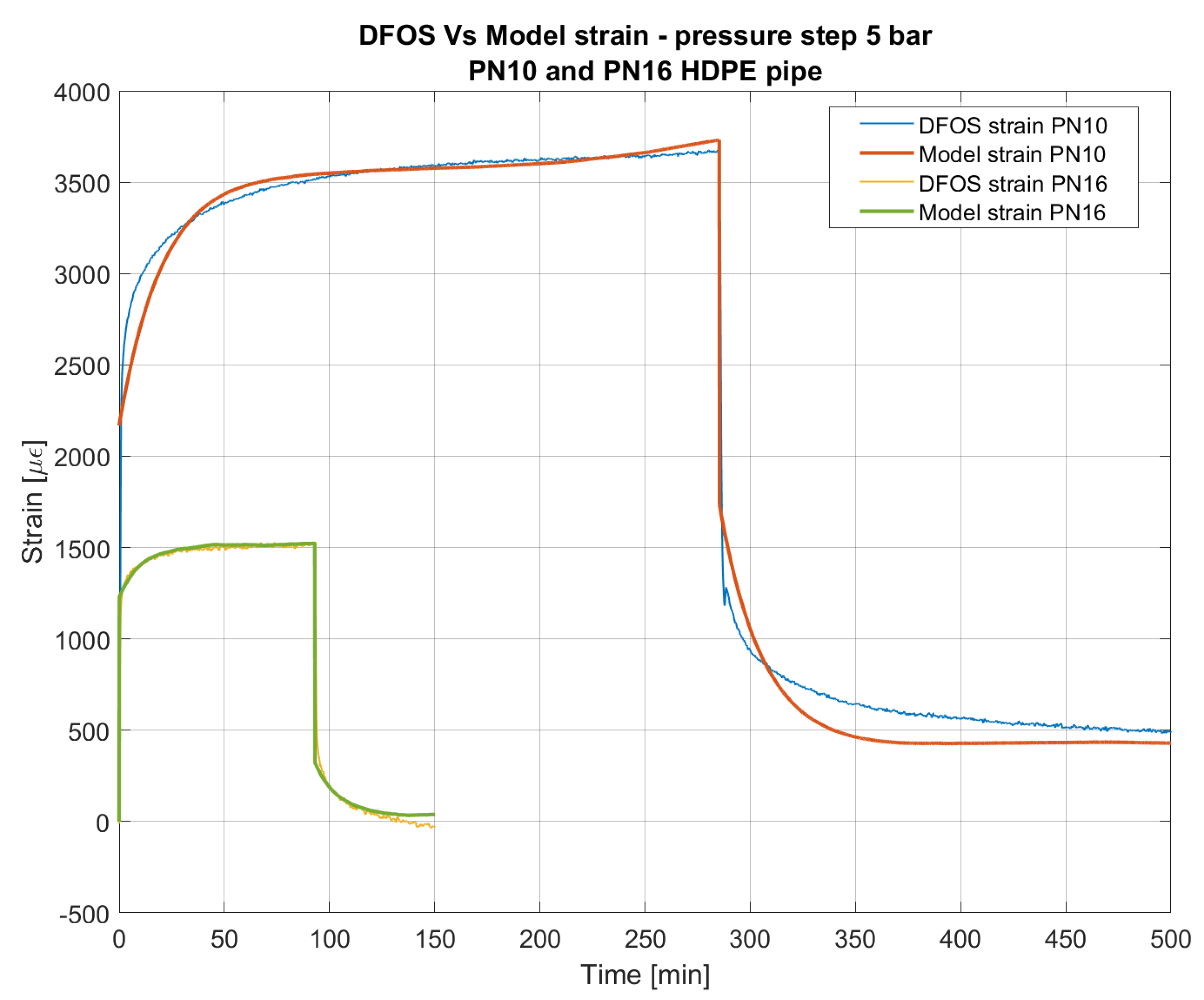
3.1. Phase I
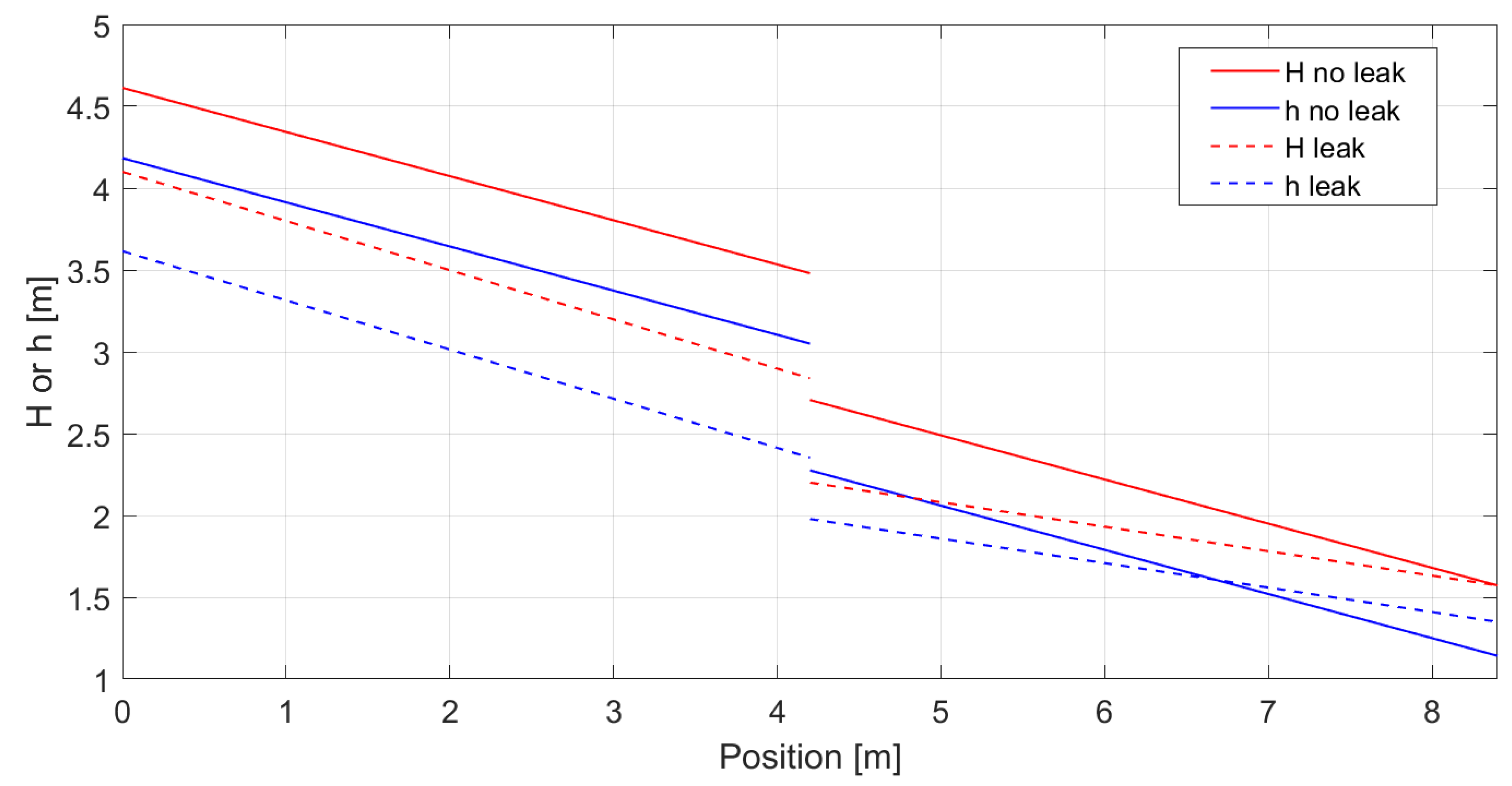
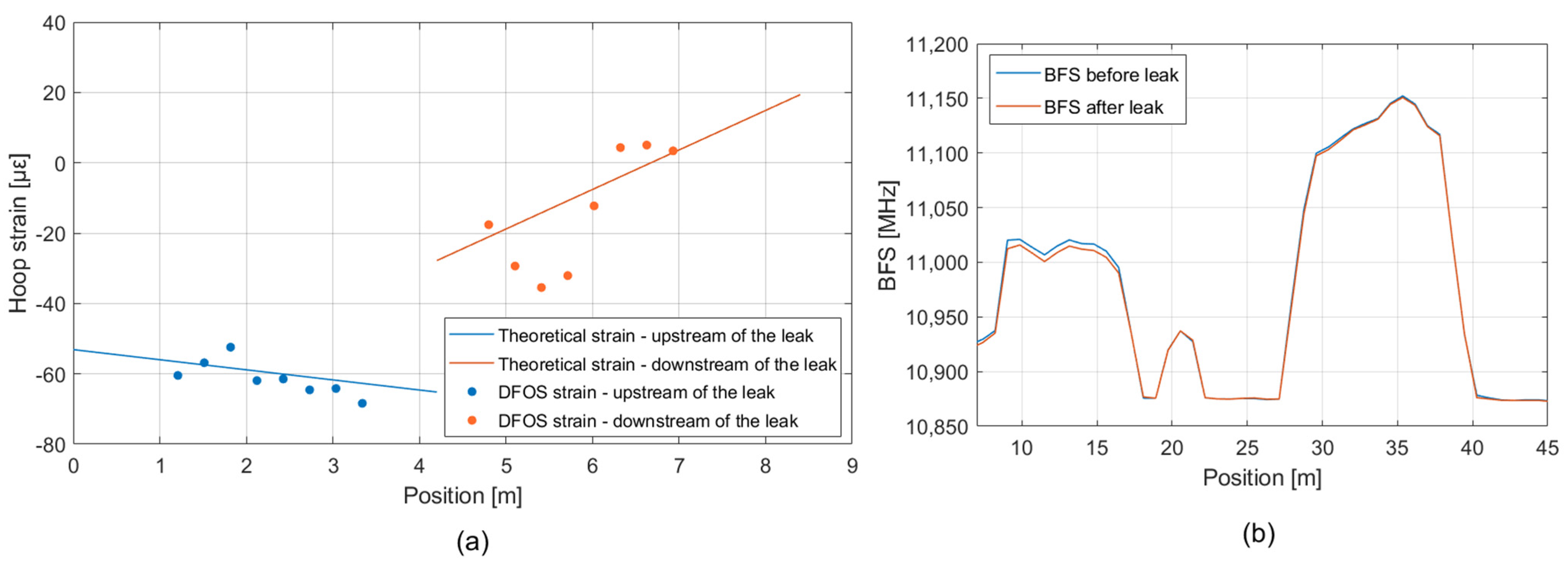
3.2. Phase II
4. Discussion and Conclusions
Author Contributions
Funding
Institutional Review Board Statement
Data Availability Statement
Acknowledgments
Conflicts of Interest
References
- Frederick, K.D.; Major, D.C. Climate change and water resources. Clim. Chang. 1997, 37, 7–23. [Google Scholar] [CrossRef]
- Farley, M.; Wyeth, G.; Ghazali, Z.B.M.; Istandar, A.; Singh, S.; Dijk, N.; Raksakulthai, V.; Kirkwood, E. The Manager’s Non-Revenue Water Handbook: A Guide to Understanding Water Losses; Ranhill Utilities Berhad; The United States Agency for International Development: Bangkok, Thailand, 2008.
- Al-washali, T.; Sharma, S.; Kennedy, M. Methods of assessment of water losses in water supply systems: A review. Water Resour. Manag. 2016, 30, 4985–5001. [Google Scholar] [CrossRef]
- Barton, N.A.; Farewell, T.S.; Hallett, S.H.; Acland, T.F. Improving pipe failure predictions: Factors affecting pipe failure in drinking water networks. Water Res. 2019, 164, 114926. [Google Scholar] [CrossRef]
- Martínez-Codina, Á.; Castillo, M.; González-Zeas, D.; Garrote, L. Pressure as a predictor of occurrence of pipe breaks in water distribution networks. Urban Water J. 2016, 13, 676–686. [Google Scholar] [CrossRef]
- Laucelli, D.; Rajani, B.; Kleiner, Y.; Giustolisi, O. Study on relationships between climate-related covariates and pipe bursts using evolutionary-based modelling. J. Hydroinform. 2014, 16, 743–757. [Google Scholar] [CrossRef]
- Adamkowski, A. Case study: Lapino powerplant penstock failure. J. Hydraul. Eng. 2001, 127, 547–555. [Google Scholar] [CrossRef]
- BenSaleh, M.S.; Qasim, S.M.; Obeid, A.M.; Garcia-Ortiz, A. A review on wireless sensor network for water pipeline monitoring applications. In Proceedings of the 2013 International Conference on Collaboration Technologies and Systems (CTS), San Diego, CA, USA, 20–24 May 2013; IEEE: Piscataway, NJ, USA, 2013; pp. 128–131. [Google Scholar]
- Bimpas, M.; Amditis, A.; Uzunoglu, N. Detection of water leaks in supply pipes using continuous wave sensor operating at 2.45 GHz. J. Appl. Geophys. 2010, 70, 226–236. [Google Scholar] [CrossRef]
- Ayadi, A.; Ghorbel, O.; BenSalah, M.S.; Abid, M. A framework of monitoring water pipeline techniques based on sensors technologies. J. King Saud Univ. Comput. Inf. Sci. 2022, 34, 47–57. [Google Scholar] [CrossRef]
- Aamo, O.M. Leak detection, size estimation and localization in pipe flows. IEEE Trans. Automat. Contr. 2015, 61, 246–251. [Google Scholar] [CrossRef]
- Ullah, N.; Ahmed, Z.; Kim, J.-M. Pipeline Leakage Detection Using Acoustic Emission and Machine Learning Algorithms. Sensors 2023, 23, 3226. [Google Scholar] [CrossRef]
- López-Higuera, J.M.; Cobo, L.R.; Incera, A.Q.; Cobo, A. Fiber optic sensors in structural health monitoring. J. Light. Technol. 2011, 29, 587–608. [Google Scholar] [CrossRef]
- Ho, M.; El-Borgi, S.; Patil, D.; Song, G. Inspection and monitoring systems subsea pipelines: A review paper. Struct. Health Monit. 2020, 19, 606–645. [Google Scholar] [CrossRef] [Green Version]
- Ren, L.; Jia, Z.; Ho, M.S.C.; Yi, T.; Li, H. Application of fiber Bragg grating based strain sensor in pipeline vortex-induced vibration measurement. Sci. China Technol. Sci. 2014, 57, 1714–1720. [Google Scholar] [CrossRef]
- Jia, Z.; Ren, L.; Li, H.; Ho, S.; Song, G. Experimental study of pipeline leak detection based on hoop strain measurement. Struct. Control Health Monit. 2015, 22, 799–812. [Google Scholar] [CrossRef]
- Barrias, A.; Casas, J.R.; Villalba, S. A review of distributed optical fiber sensors for civil engineering applications. Sensors 2016, 16, 748. [Google Scholar] [CrossRef] [PubMed] [Green Version]
- Hong, C.-Y.; Zhang, Y.-F.; Li, G.-W.; Zhang, M.-X.; Liu, Z.-X. Recent progress of using Brillouin distributed fiber optic sensors for geotechnical health monitoring. Sens. Actuators A Phys. 2017, 258, 131–145. [Google Scholar] [CrossRef]
- Bertulessi, M.; Bignami, D.F.; Boschini, I.; Chiarini, A.; Ferrario, M.; Mazzon, N.; Menduni, G.; Morosi, J.; Zambrini, F. Conceptualization and Prototype of an Anti-Erosion Sensing Revetment for Levee Monitoring: Experimental Tests and Numerical Modeling. Water 2020, 12, 3025. [Google Scholar] [CrossRef]
- Zhao, X.; Gong, P.; Qiao, G.; Lu, J.; Lv, X.; Ou, J. Brillouin corrosion expansion sensors for steel reinforced concrete structures using a fiber optic coil winding method. Sensors 2011, 11, 10798–10819. [Google Scholar] [CrossRef] [PubMed] [Green Version]
- Biondi, A.M.; Zhou, J.; Guo, X.; Wu, R.; Tang, Q.; Gandhi, H.; Yu, T.; Gopalan, B.; Hanna, T.; Ivey, J.; et al. Pipeline structural health monitoring using distributed fiber optic sensing textile. Opt. Fiber Technol. 2022, 70, 102876. [Google Scholar] [CrossRef]
- Galindez-Jamioy, C.A.; Lopez-Higuera, J.M. Brillouin distributed fiber sensors: An overview and applications. J. Sens. 2012, 2012, 204121. [Google Scholar] [CrossRef] [Green Version]
- Wang, C.; Olson, M.; Sherman, B.; Dorjkhand, N.; Mehr, J.; Singh, S. Reliable leak detection in pipelines using integrated DdTS temperature and DAS acoustic fiber-optic sensor. In Proceedings of the 2018 International Carnahan Conference on Security Technology (ICCST), Montreal, QC, Canada, 22–25 October 2018; IEEE: Piscataway, NJ, USA, 2018; pp. 1–5. [Google Scholar]
- Stajanca, P.; Chruscicki, S.; Homann, T.; Seifert, S.; Schmidt, D.; Habib, A. Detection of leak-induced pipeline vibrations using fiber—Optic distributed acoustic sensing. Sensors 2018, 18, 2841. [Google Scholar] [CrossRef] [Green Version]
- Niklès, M.; Vogel, B.H.; Briffod, F.; Grosswig, S.; Sauser, F.; Luebbecke, S.; Bals, A.; Pfeiffer, T. Leakage detection using fiber optics distributed temperature monitoring. In Smart Structures and Materials 2004: Smart Sensor Technology and Measurement Systems; SPIE: Bellingham, WA, USA, 2004; pp. 18–25. [Google Scholar]
- Prisutova, J.; Krynkin, A.; Tait, S.; Horoshenkov, K. Use of fibre-optic sensors for pipe condition and hydraulics measurements: A review. CivilEng 2022, 3, 85–113. [Google Scholar] [CrossRef]
- Bernini, R.; Minardo, A.; Zeni, L. Vectorial dislocation monitoring of pipelines by use of Brillouin-based fiber-optics sensors. Smart Mater. Struct. 2007, 17, 015006. [Google Scholar] [CrossRef]
- Ren, L.; Jiang, T.; Jia, Z.; Li, D.; Yuan, C.; Li, H. Pipeline corrosion and leakage monitoring based on the distributed optical fiber sensing technology. Measurement 2018, 122, 57–65. [Google Scholar] [CrossRef]
- Twort, A.C.; Ratnayaka, D.D.; Brandt, M.J. Water Supply; Elsevier: Amsterdam, The Netherlands, 2000. [Google Scholar]
- Ruchti, G.F. Water Pipeline Condition Assessment; American Society of Civil Engineers (ASCE): Reston, VA, USA, 2017. [Google Scholar]
- Bastianini, F.; Di Sante, R.; Falcetelli, F.; Marini, D.; Bolognini, G. Optical fiber sensing cables for Brillouin-based distributed measurements. Sensors 2019, 19, 5172. [Google Scholar] [CrossRef] [PubMed] [Green Version]
- Feng, C.; Kadum, J.E.; Schneider, T. The State-of-the-Art of Brillouin Distributed Fiber Sensing; IntechOpen: London, UK, 2019. [Google Scholar]
- Diaz, S.; Mafang, S.F.; Lopez-Amo, M.; Thévenaz, L. A high-performance optical time-domain Brillouin distributed fiber sensor. IEEE Sens. J. 2008, 8, 1268–1272. [Google Scholar] [CrossRef]
- Zou, W.; He, Z.; Hotate, K. Complete discrimination of strain and temperature using Brillouin frequency shift and birefringence in a polarization-maintaining fiber. Opt. Express 2009, 17, 1248–1255. [Google Scholar] [CrossRef]
- Lanticq, V.; Quiertant, M.; Merliot, E.; Delepine-Lesoille, S. Brillouin sensing cable: Design and experimental validation. IEEE Sens. J. 2008, 8, 1194–1201. [Google Scholar] [CrossRef]
- Bertulessi, M.; Bignami, D.F.; Boschini, I.; Brunero, M.; Ferrario, M.; Menduni, G.; Morosi, J.; Paganone, E.J.; Zambrini, F. Monitoring Strategic Hydraulic Infrastructures by Brillouin Distributed Fiber Optic Sensors. Water 2022, 14, 188. [Google Scholar] [CrossRef]
- Petrucci, G. Lezioni di Costruzione di Macchine; Dipartimento Di Meccanica E Aeronautica: Palermo, Italy, 2002. [Google Scholar]
- Elleuch, R.; Taktak, W. Viscoelastic behavior of HDPE polymer using tensile and compressive loading. J. Mater. Eng. Perform. 2006, 15, 111–116. [Google Scholar] [CrossRef]
- Fathi-Moghadam, M.; Kiani, S. Simulation of transient flow in viscoelastic pipe networks. J. Hydraul. Res. 2019, 58, 531–540. [Google Scholar] [CrossRef]
- Majda, P.; Skrodzewicz, J. A modified creep model of epoxy adhesive at ambient temperature. Int. J. Adhes. Adhes. 2009, 29, 396–404. [Google Scholar] [CrossRef]
- Colebrook, C.F.; White, C.M. Experiments with fluid friction in roughened pipes. Proc. R. Soc. Lond. 1937, 161, 367–381. [Google Scholar] [CrossRef]
- Li, J.; Dasgupta, A. Failure-mechanism models for creep and creep rupture. IEEE Trans. Reliab. 1993, 42, 339–353. [Google Scholar] [CrossRef]


| Phase | [m] | S [m] | Δ [m] | Δν [GHz] | [MHz] | [s] | |
|---|---|---|---|---|---|---|---|
| I | 0.198 | 0.05 | 0.45 | 10.4–11.4 | 5 | 256 | 7 |
| II | 0.108 | 0.04 | 0.72 | 10.75–11.3 | 1 | 256 | 20 |
| Parameter | u.m. | PN10 | PN16 | PN25 |
|---|---|---|---|---|
| β | - | 0.86 | 0.78 | 0.70 |
| ν | - | 0.4 | 0.4 | 0.4 |
| MPa | 1.05 × 10³ | 1.05 × 10³ | 1.05 × 10³ | |
| MPa | 1.65 × 10³ | 4.47 × 10³ | 4.47 × 10³ | |
| MPa s | 2.04 × 10⁶ | 2.77 × 10⁶ | 2.77 × 10⁶ | |
| MPa s | 2.13 × 10⁸ | 4.68 × 10⁸ | 4.68 × 10⁸ | |
| µε/°C | 200 | 200 | 200 | |
| - | 4 | 4 | 4 |
| Pipe | ΔJ Estimated | ΔJ Measured | Error % |
|---|---|---|---|
| Upstream of leak | −0.03 | −0.04 | 30.27 |
| Downstream of leak | +0.12 | +0.11 | 12.31 |
Disclaimer/Publisher’s Note: The statements, opinions and data contained in all publications are solely those of the individual author(s) and contributor(s) and not of MDPI and/or the editor(s). MDPI and/or the editor(s) disclaim responsibility for any injury to people or property resulting from any ideas, methods, instructions or products referred to in the content. |
© 2023 by the authors. Licensee MDPI, Basel, Switzerland. This article is an open access article distributed under the terms and conditions of the Creative Commons Attribution (CC BY) license (https://creativecommons.org/licenses/by/4.0/).
Share and Cite
Bertulessi, M.; Bignami, D.F.; Boschini, I.; Longoni, M.; Menduni, G.; Morosi, J. Experimental Investigations of Distributed Fiber Optic Sensors for Water Pipeline Monitoring. Sensors 2023, 23, 6205. https://doi.org/10.3390/s23136205
Bertulessi M, Bignami DF, Boschini I, Longoni M, Menduni G, Morosi J. Experimental Investigations of Distributed Fiber Optic Sensors for Water Pipeline Monitoring. Sensors. 2023; 23(13):6205. https://doi.org/10.3390/s23136205
Chicago/Turabian StyleBertulessi, Manuel, Daniele Fabrizio Bignami, Ilaria Boschini, Marina Longoni, Giovanni Menduni, and Jacopo Morosi. 2023. "Experimental Investigations of Distributed Fiber Optic Sensors for Water Pipeline Monitoring" Sensors 23, no. 13: 6205. https://doi.org/10.3390/s23136205