
Assessment of Electromagnetic Field Exposure on European Roads: A Comprehensive In Situ Measurement Campaign

Abstract
:1. Introduction
2. Materials and Methods
2.1. Measurement Equipment
2.2. Measurement Procedure
2.3. Data Acquisition, Processing, and Analysis
3. Results and Discussion
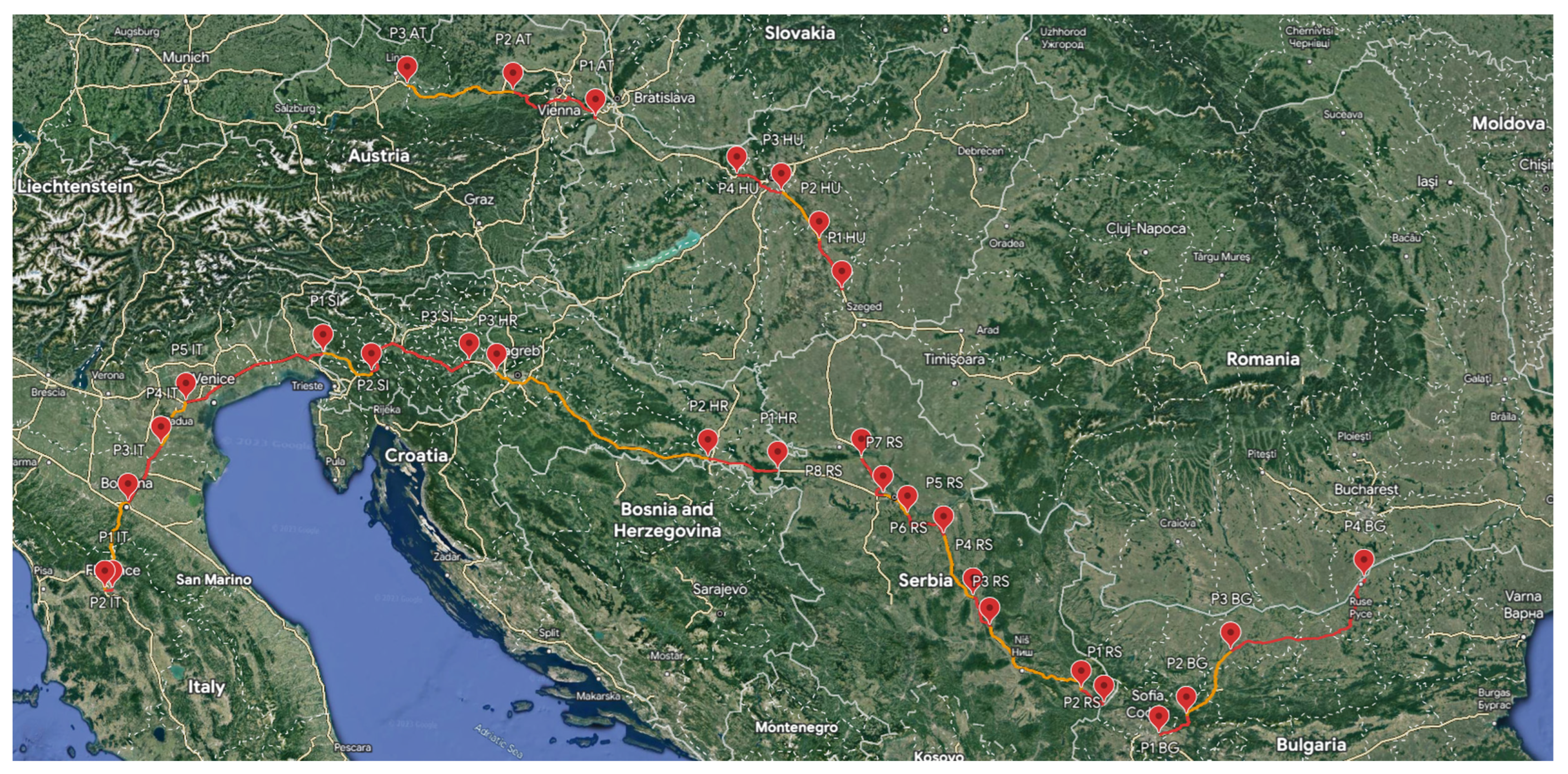
3.1. Electromagnetic Field on Different European Roads
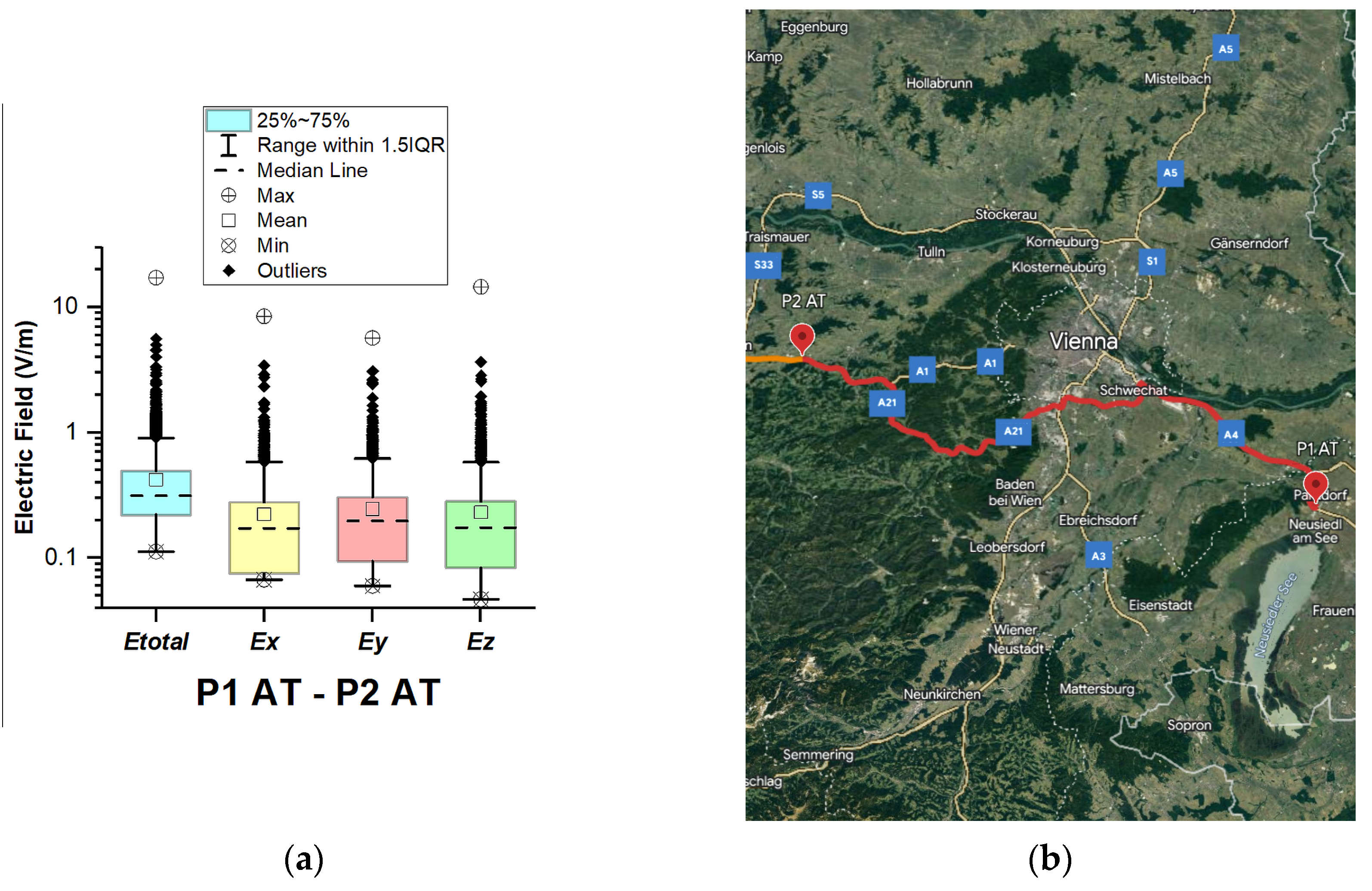
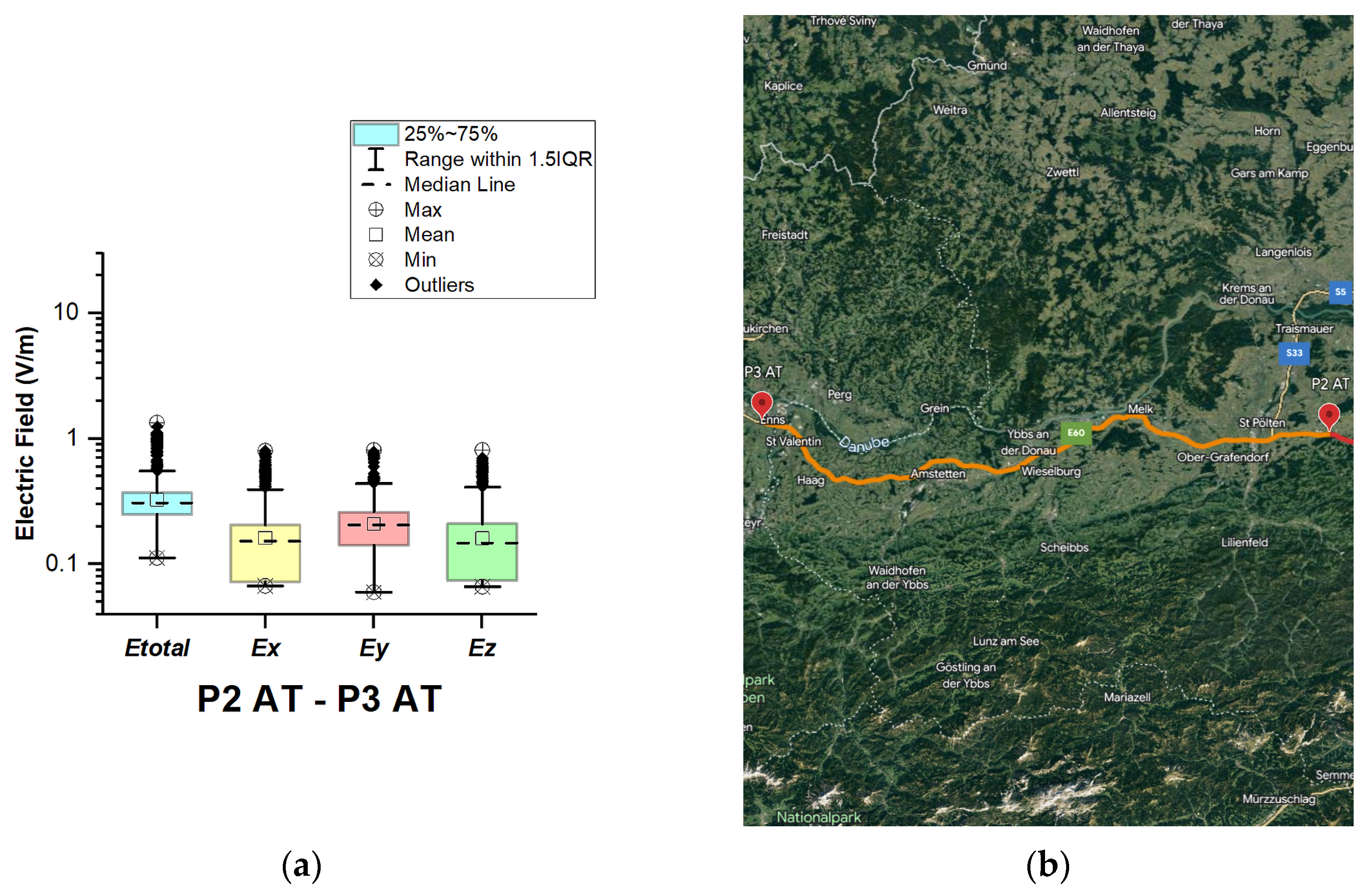
3.1.1. Austria
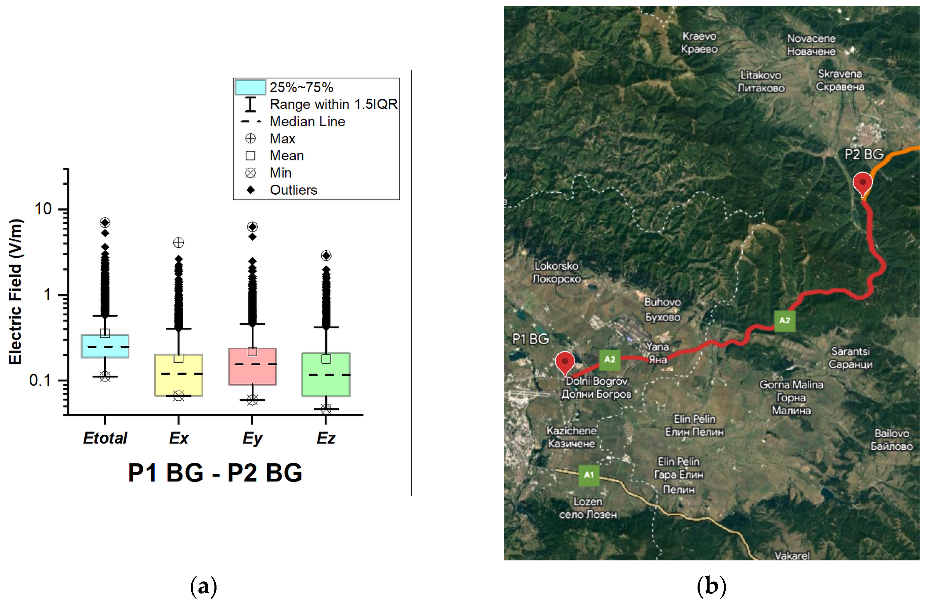
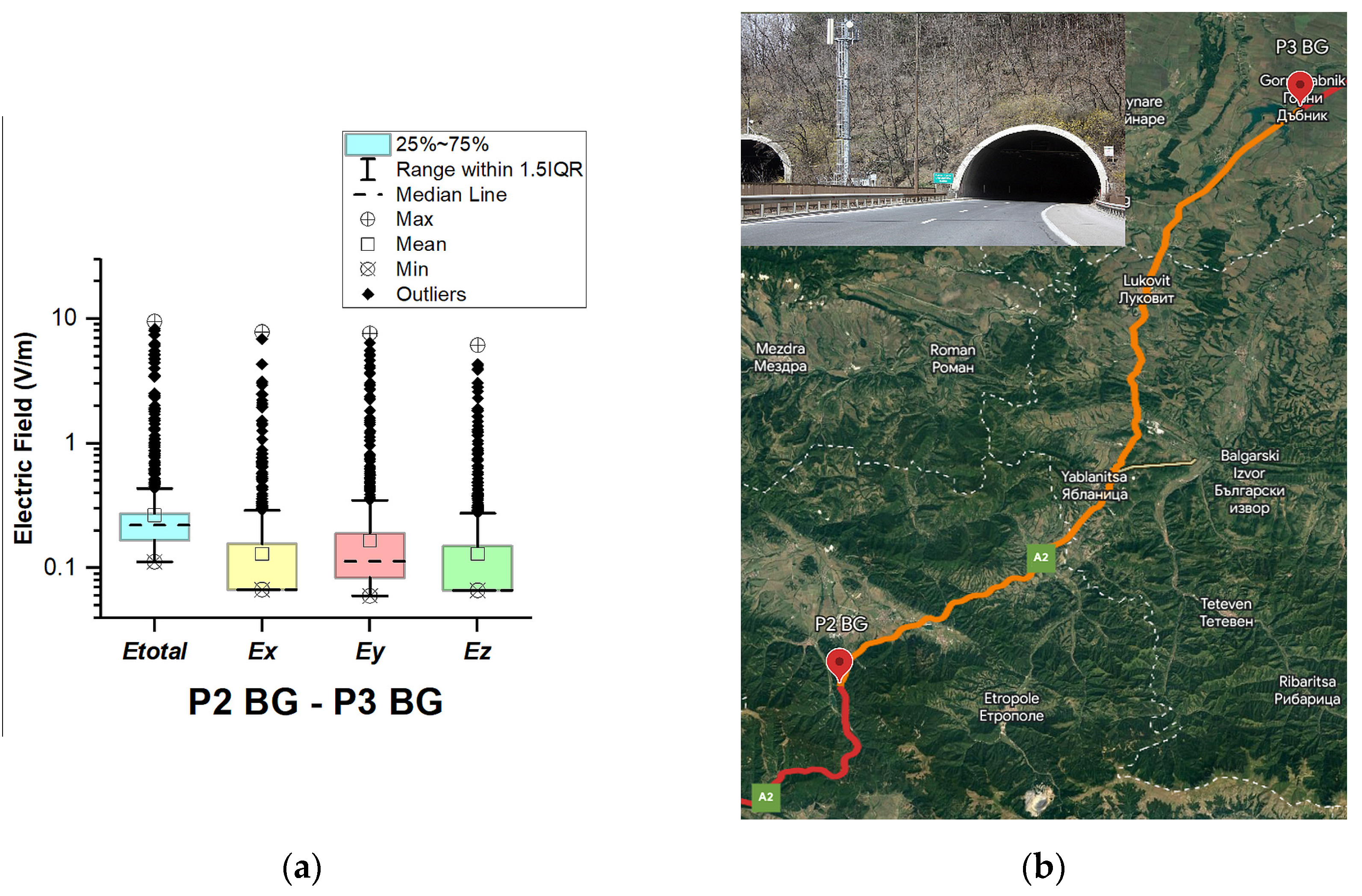
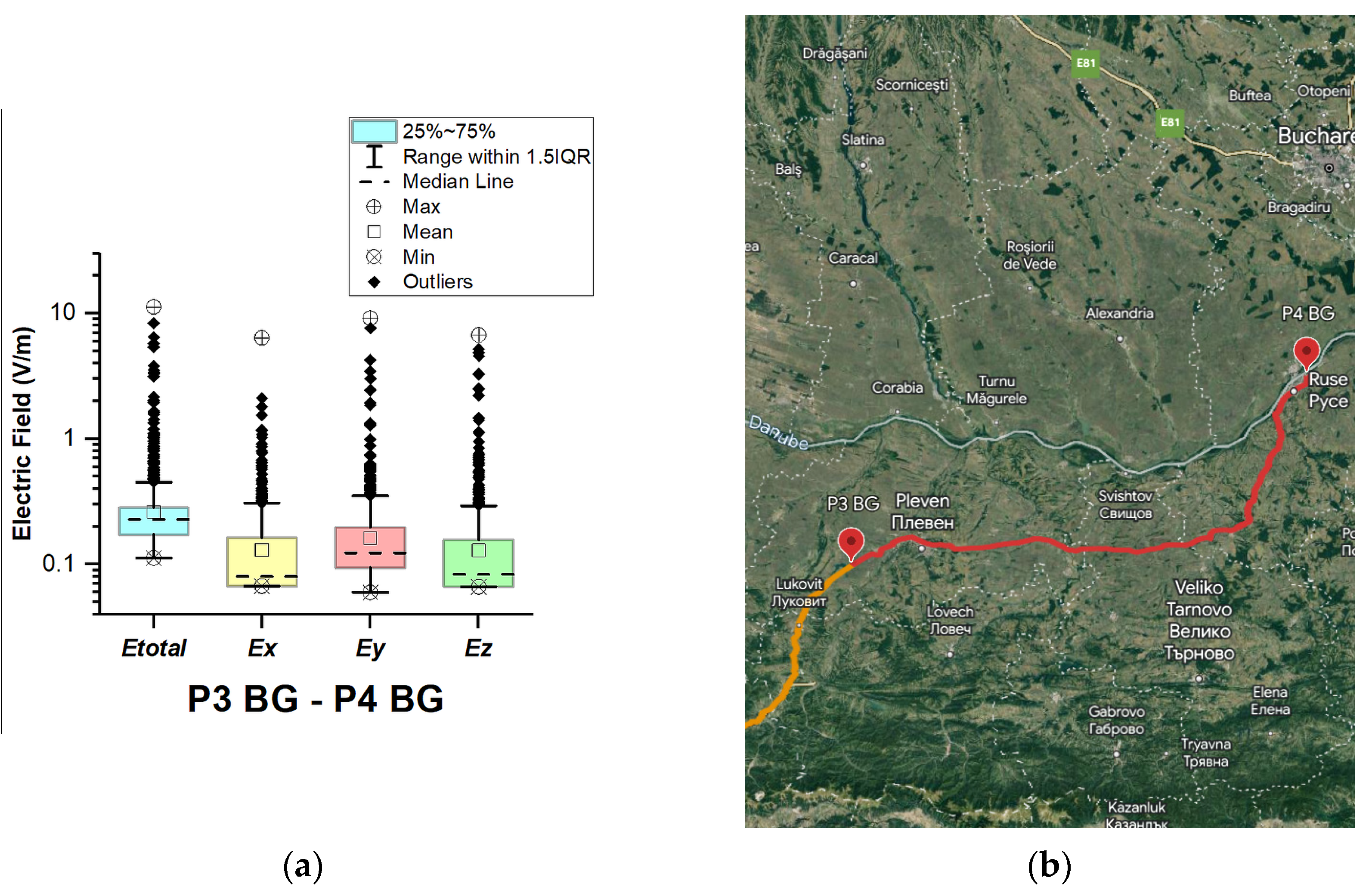
3.1.2. Bulgaria
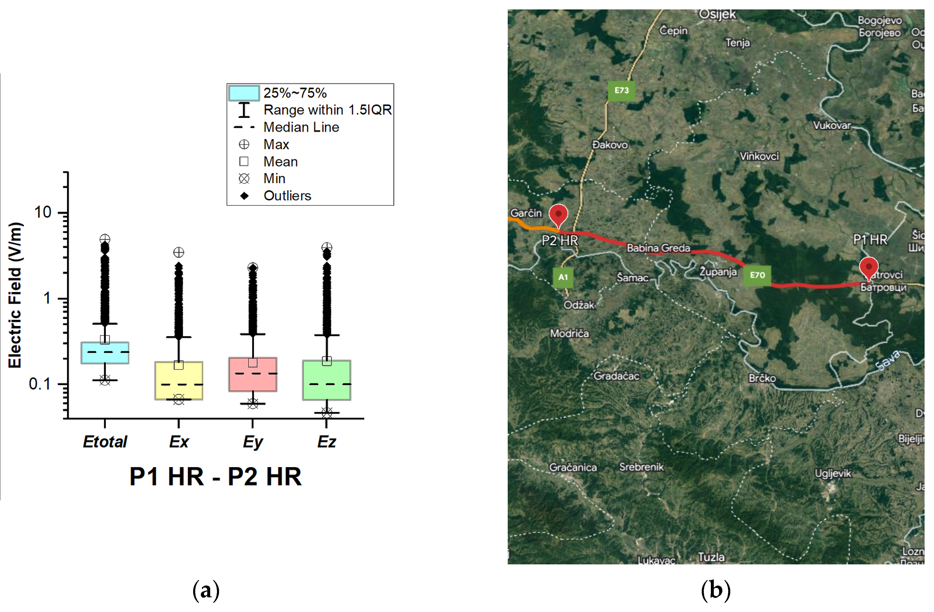
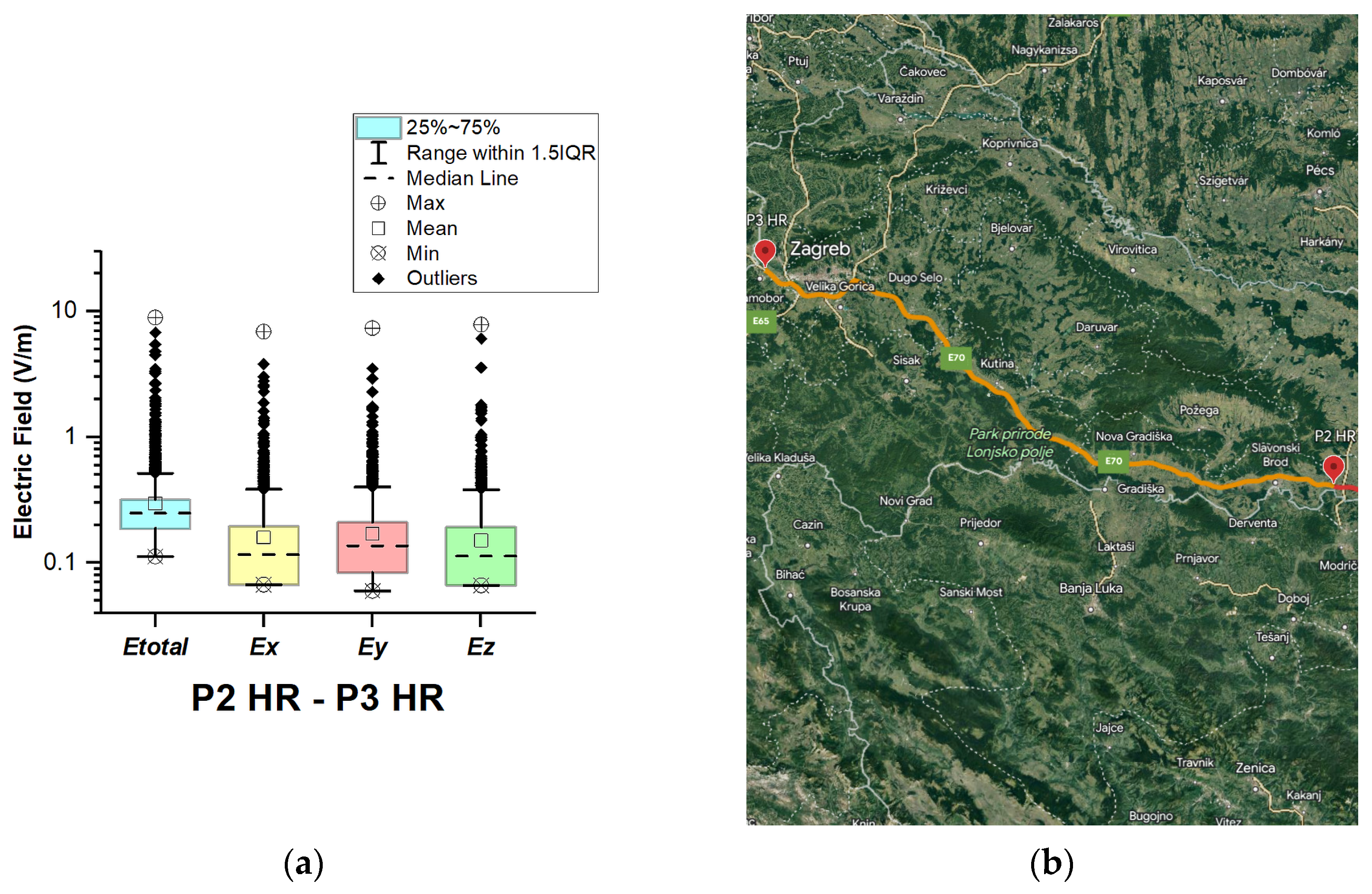
3.1.3. Croatia
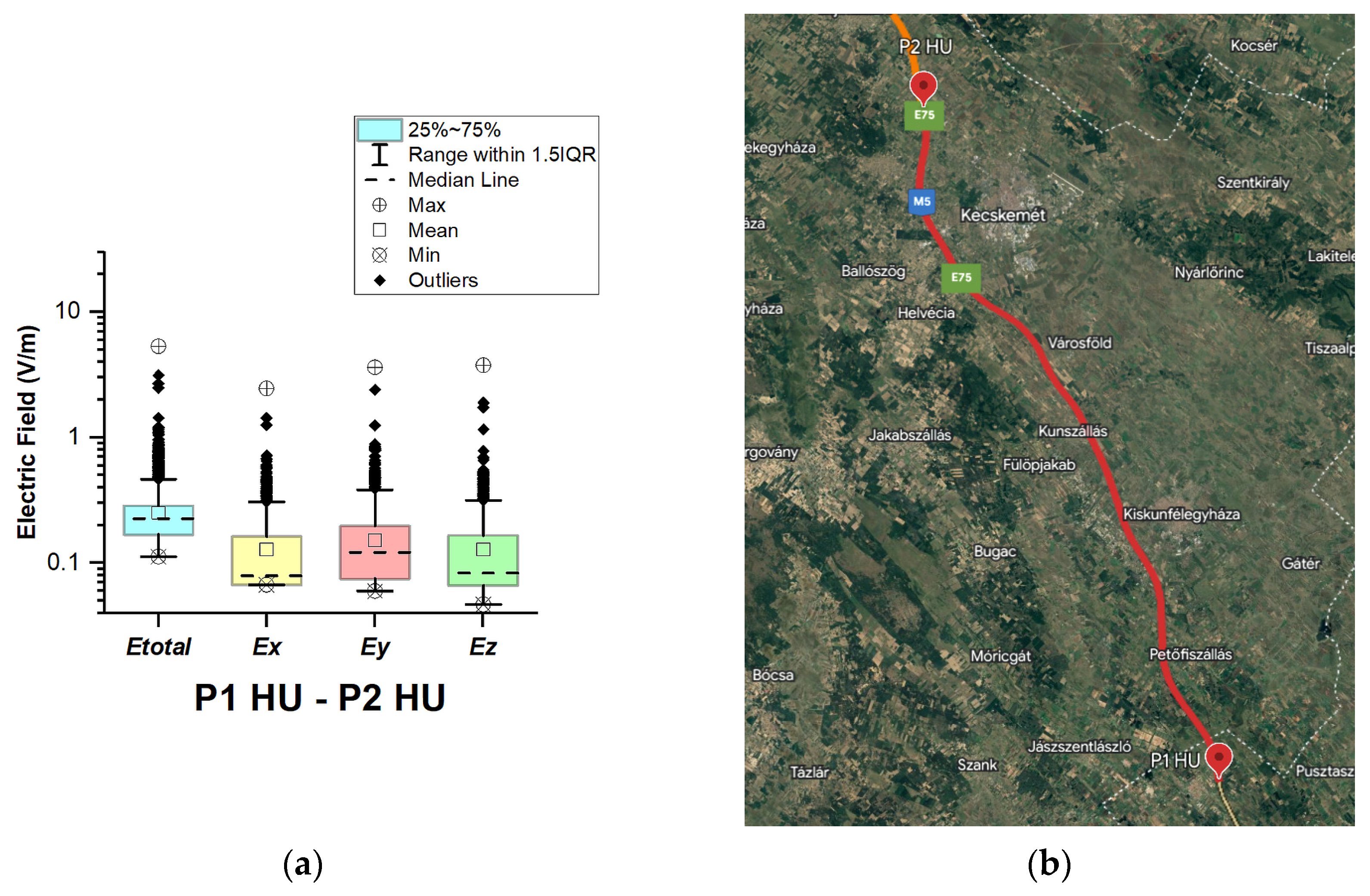
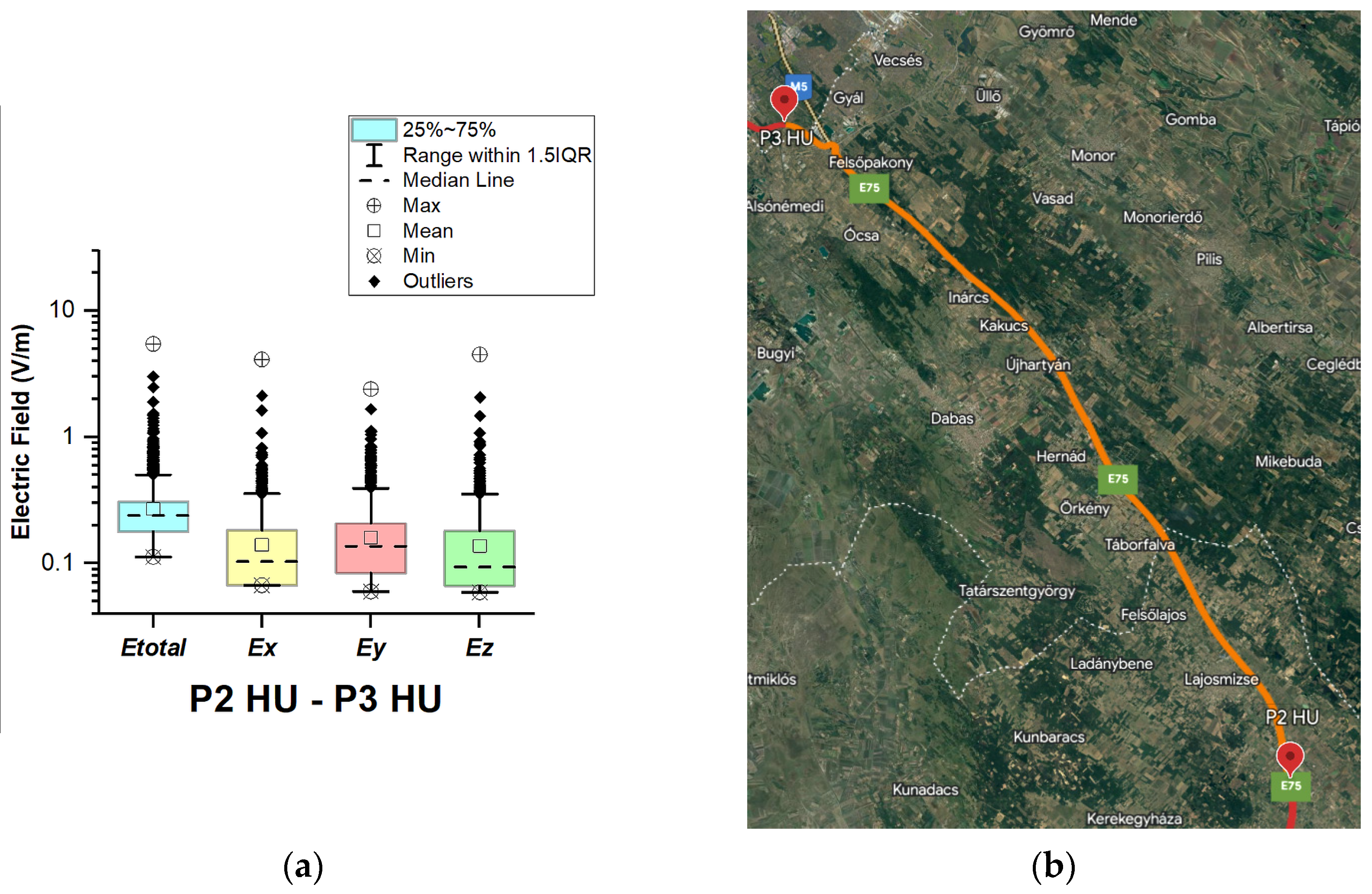
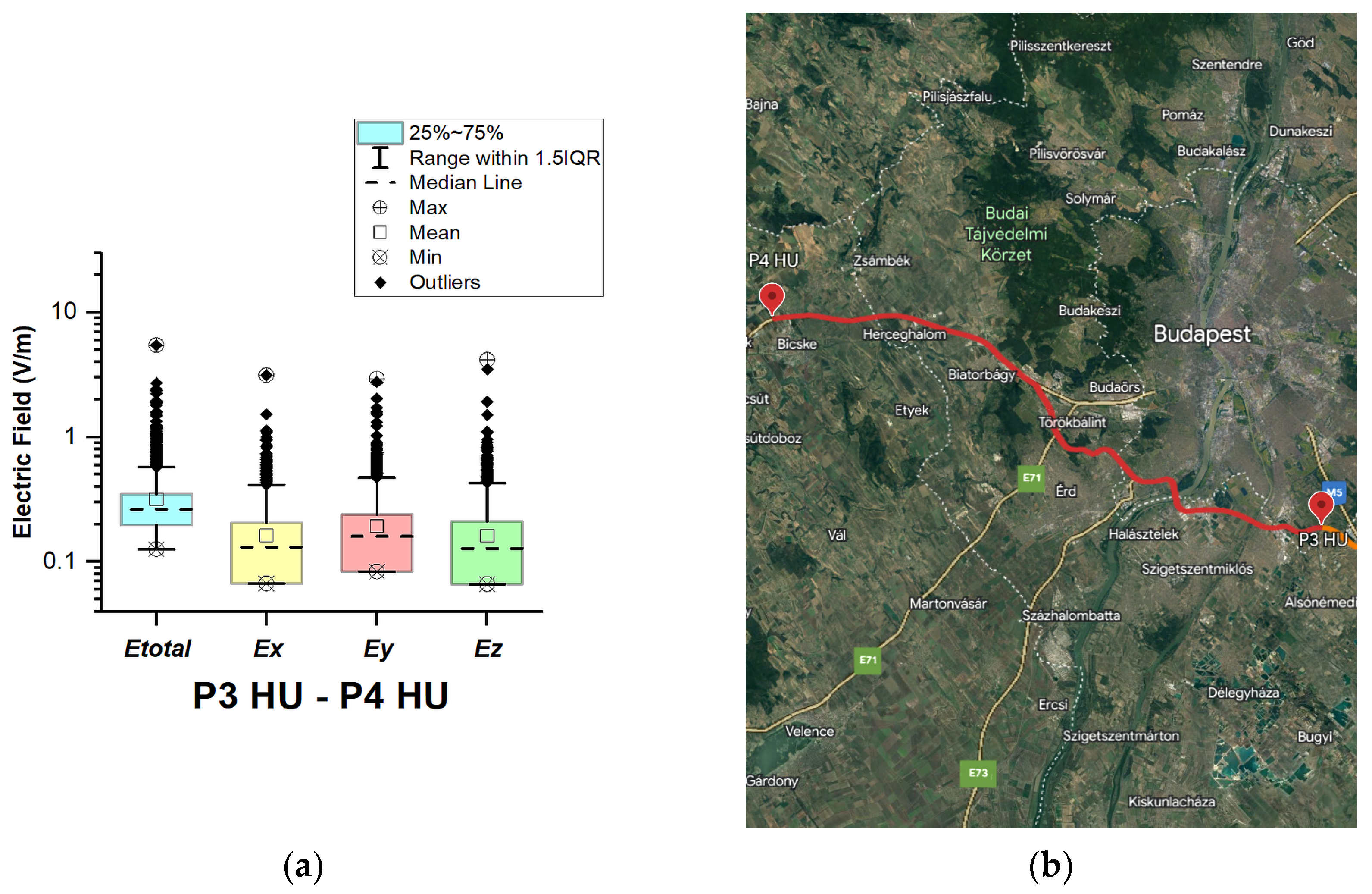
3.1.4. Hungary
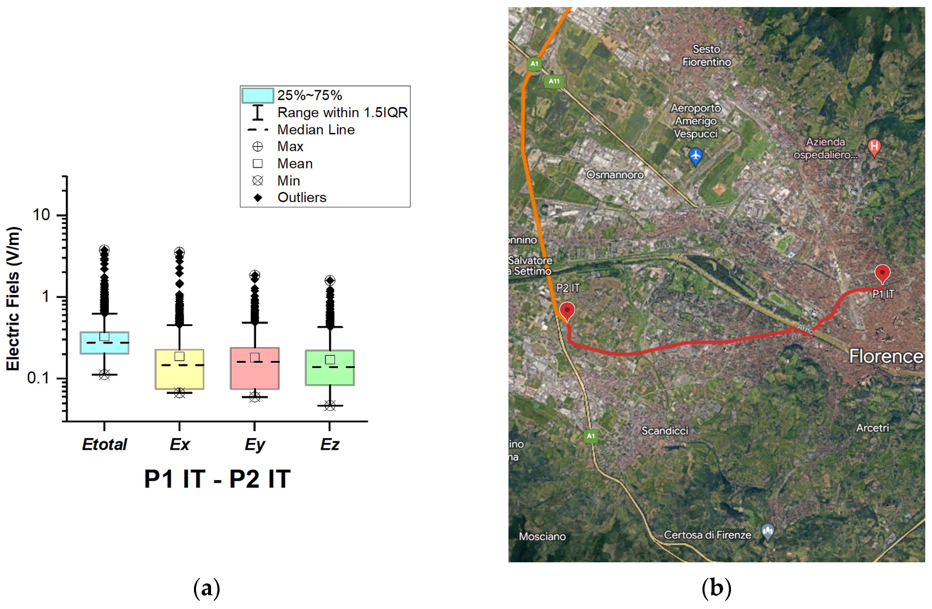
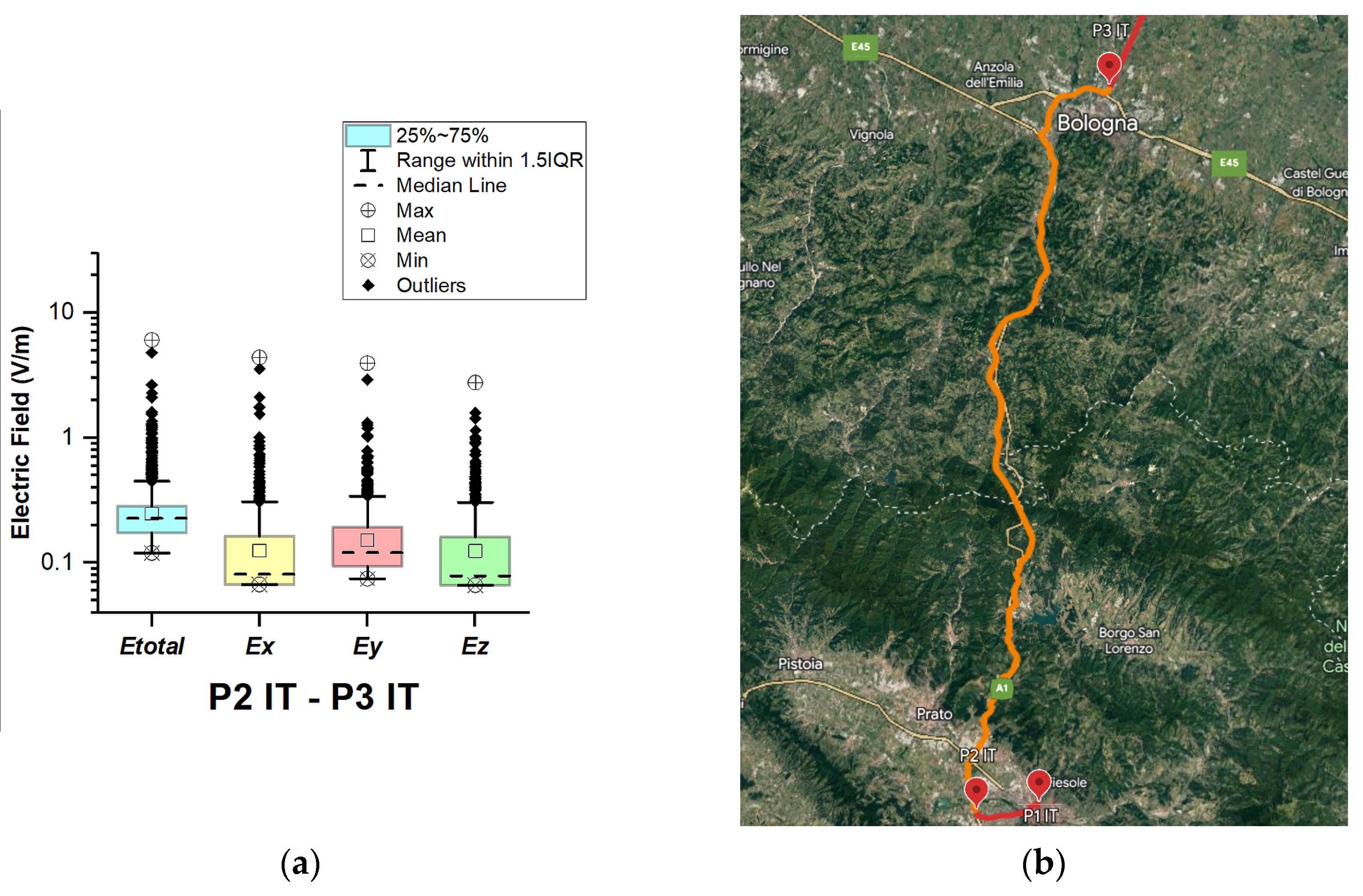
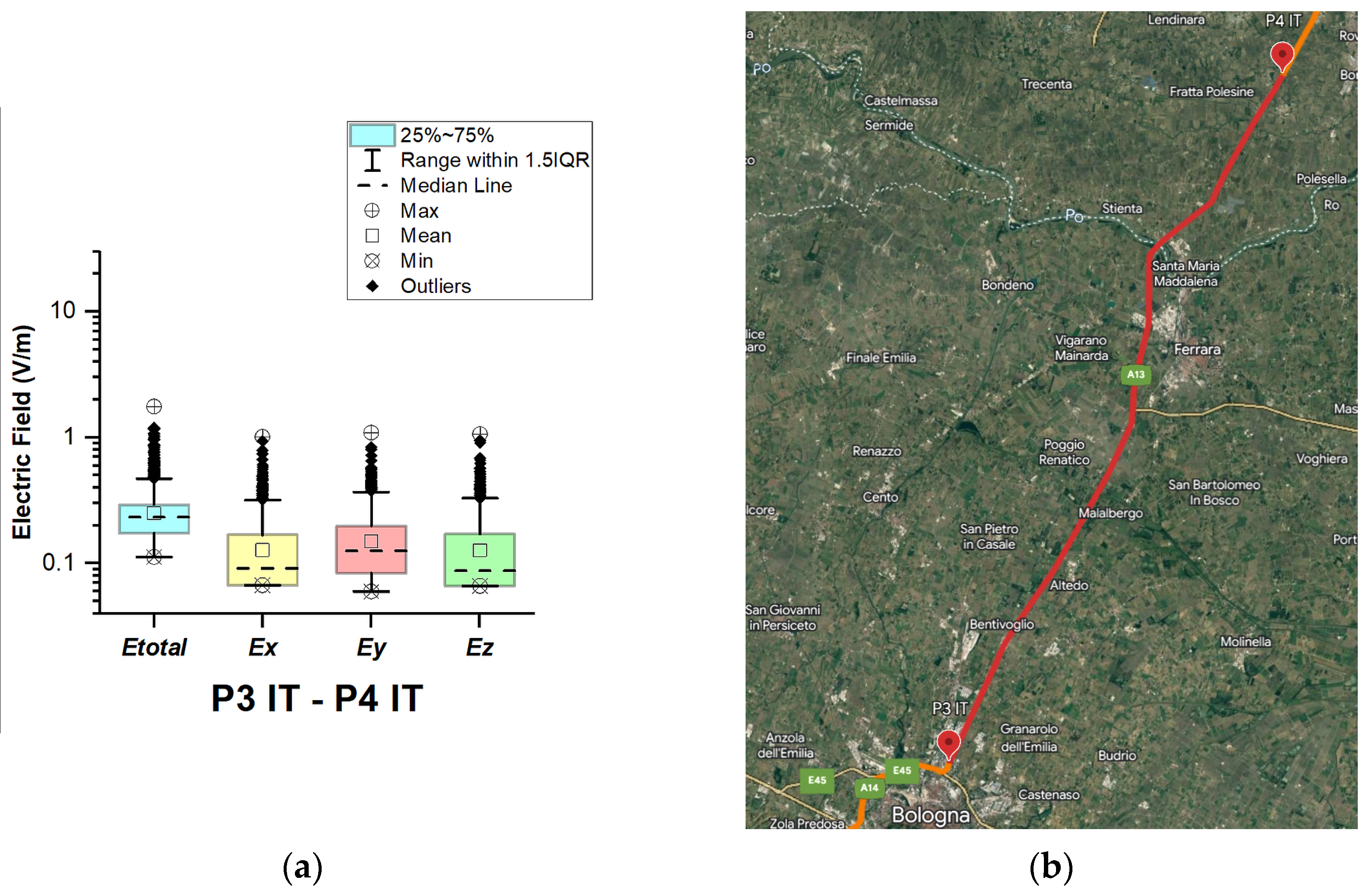
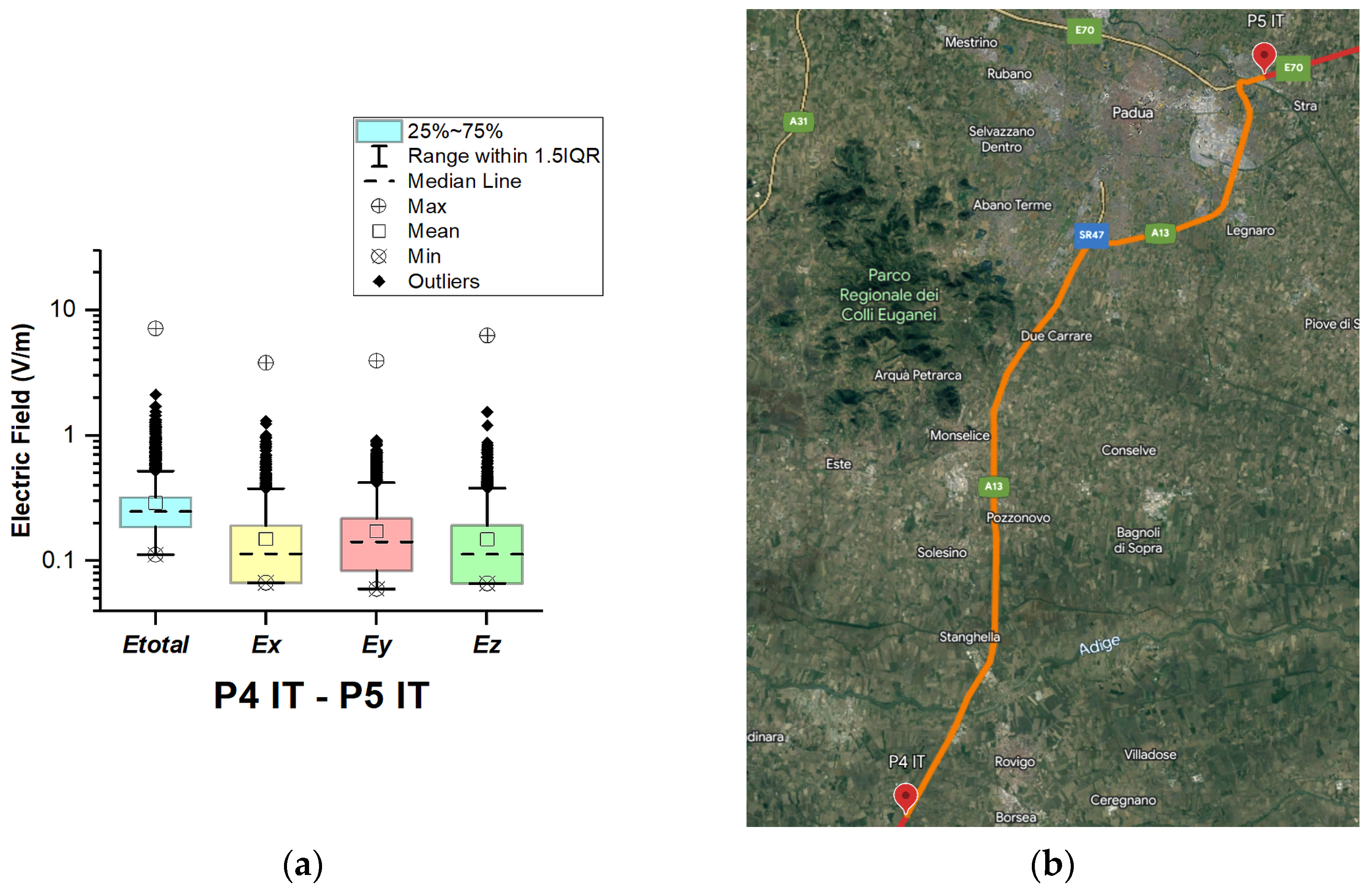
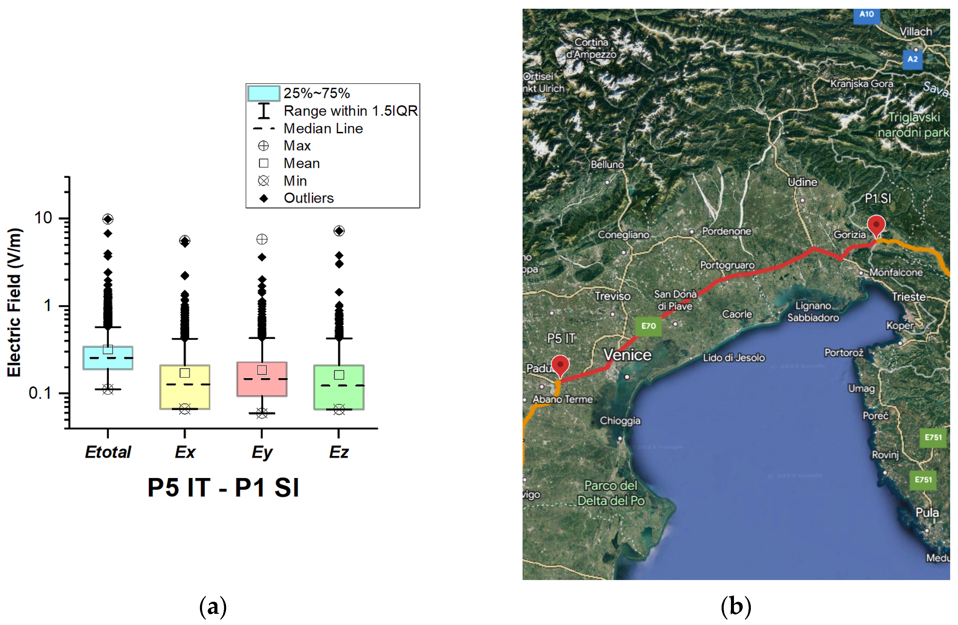
3.1.5. Italy
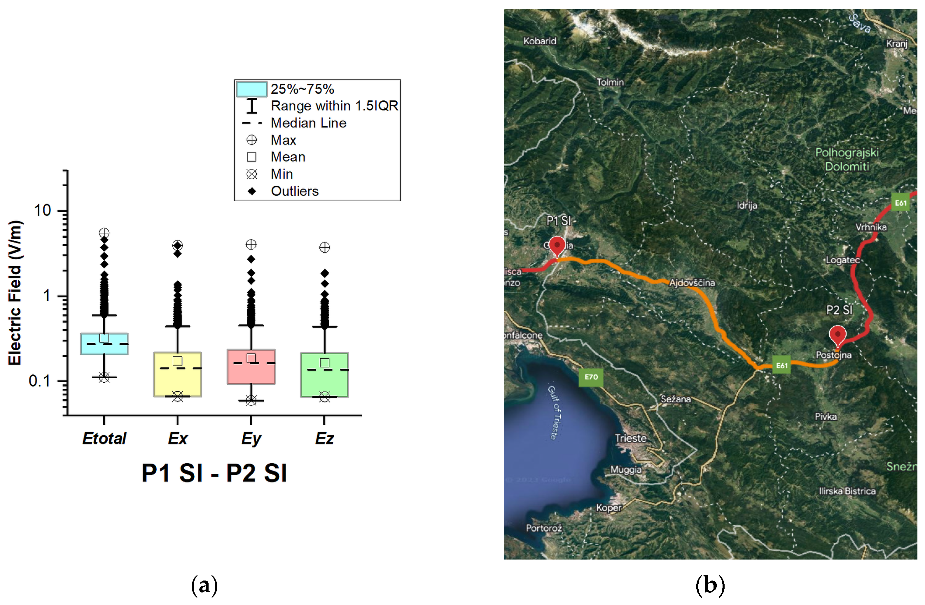
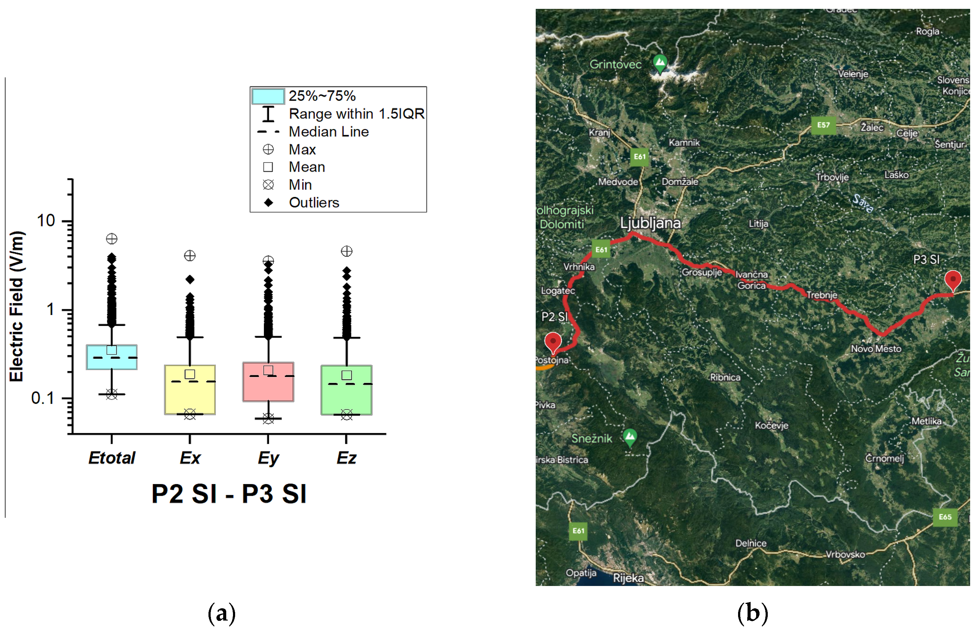
3.1.6. Slovenia
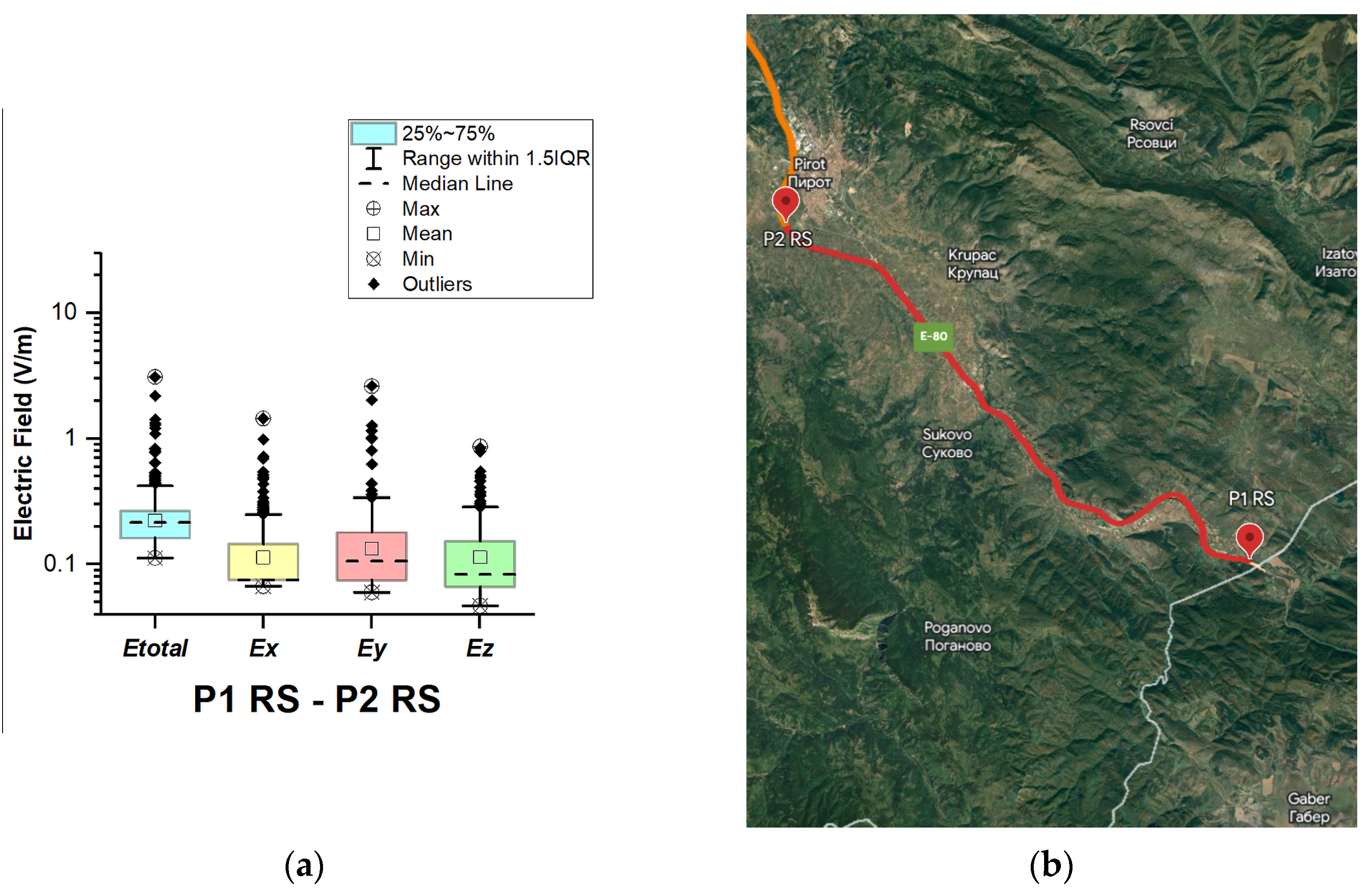
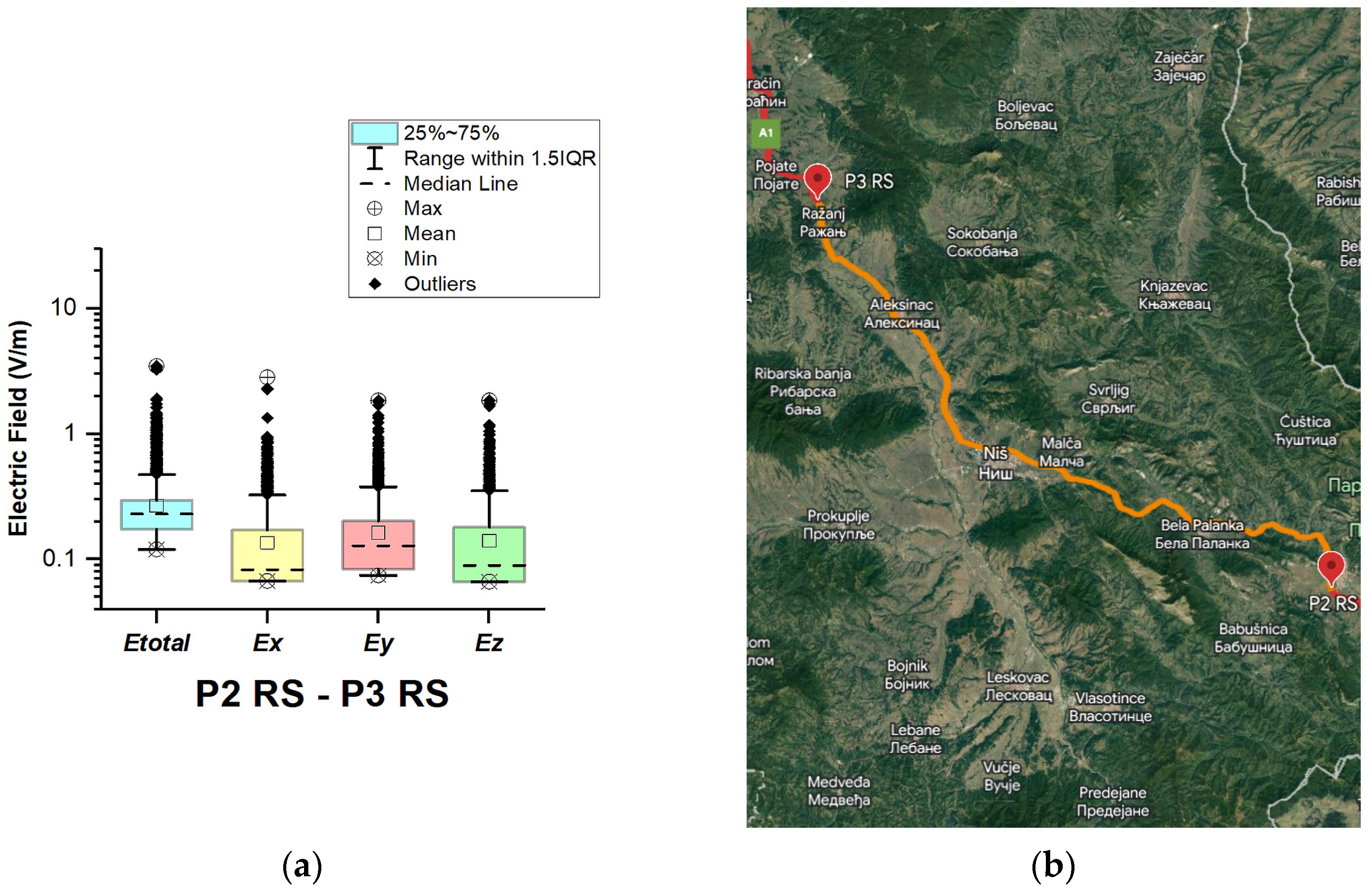
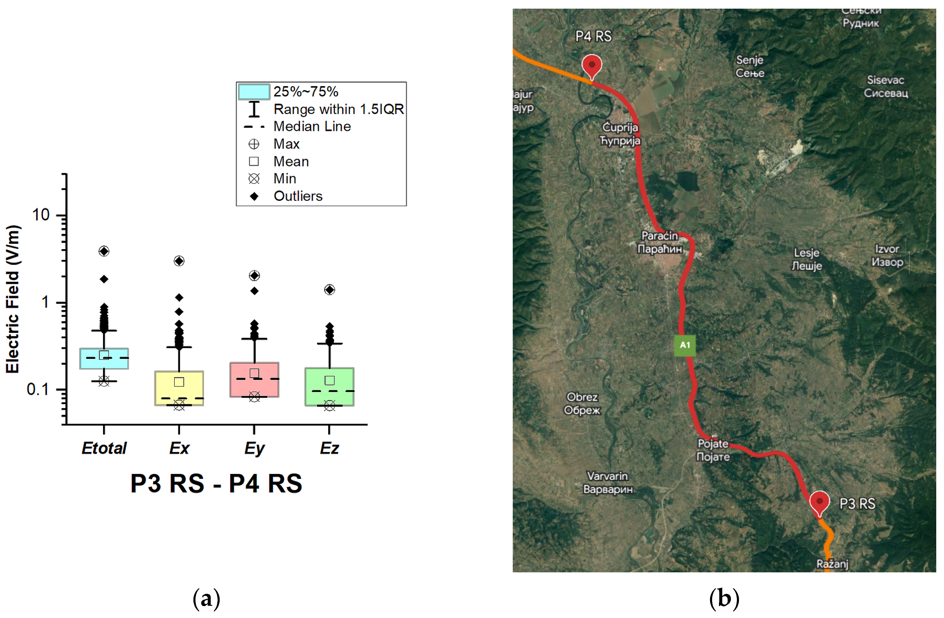
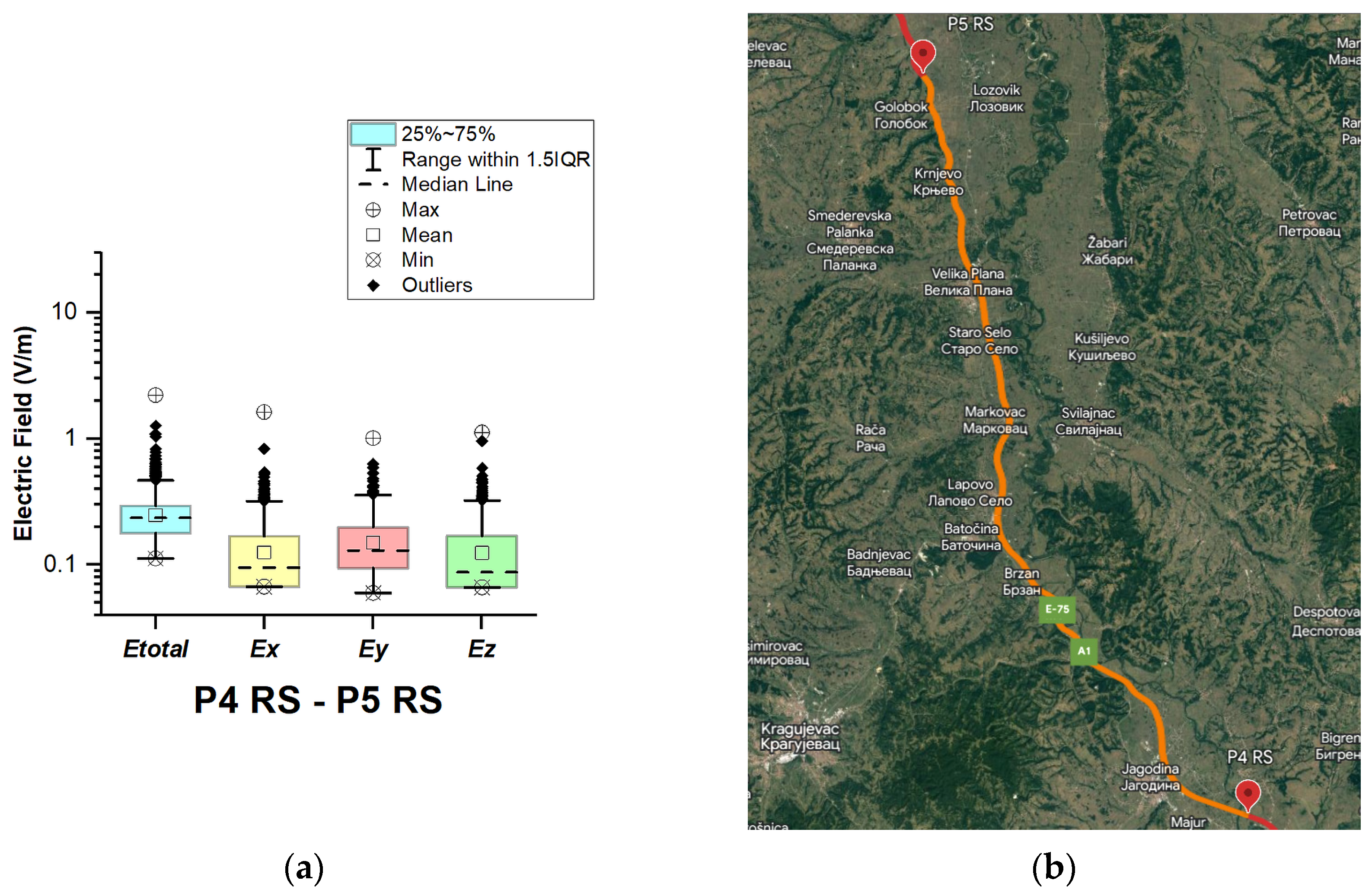
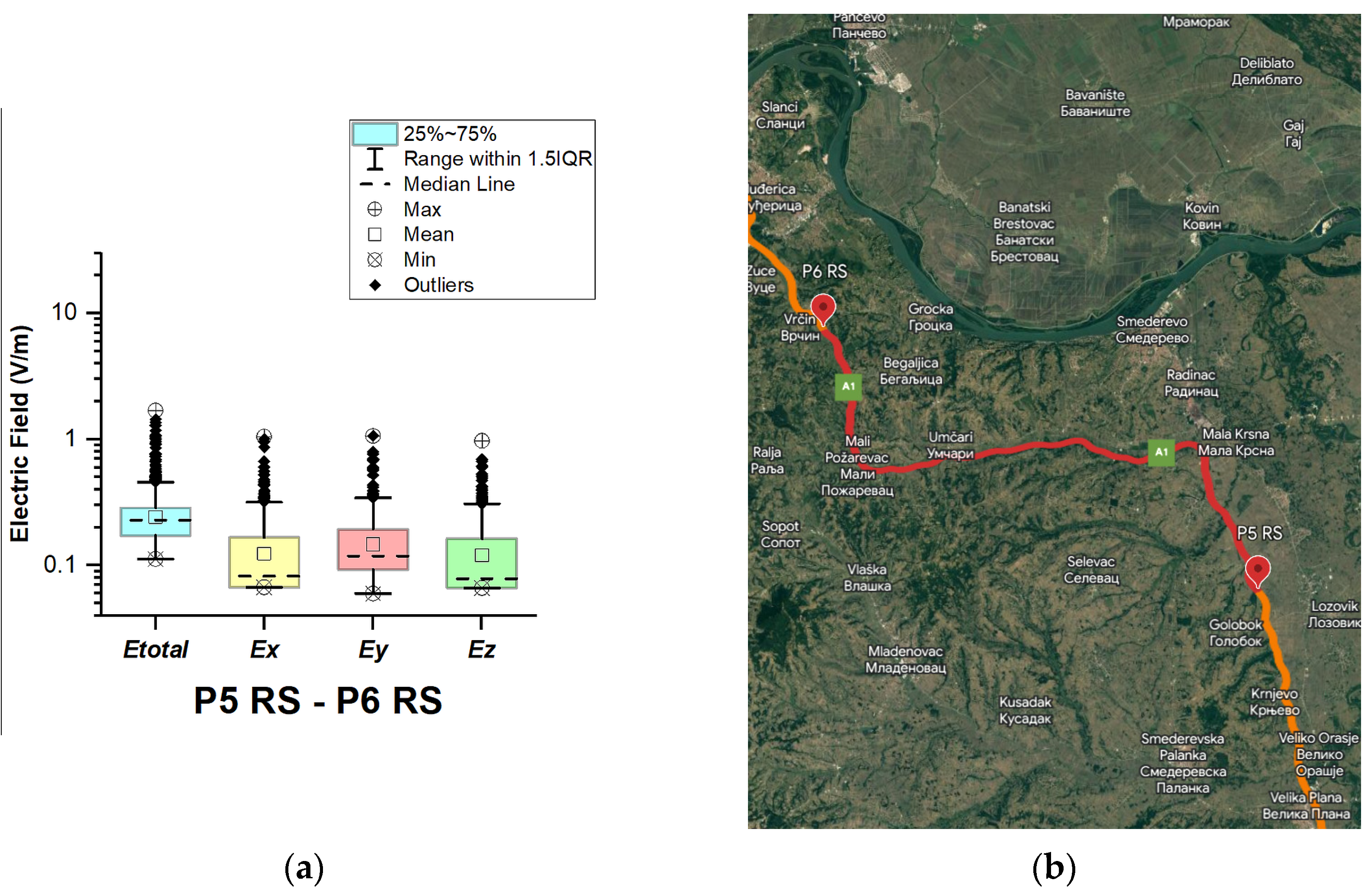
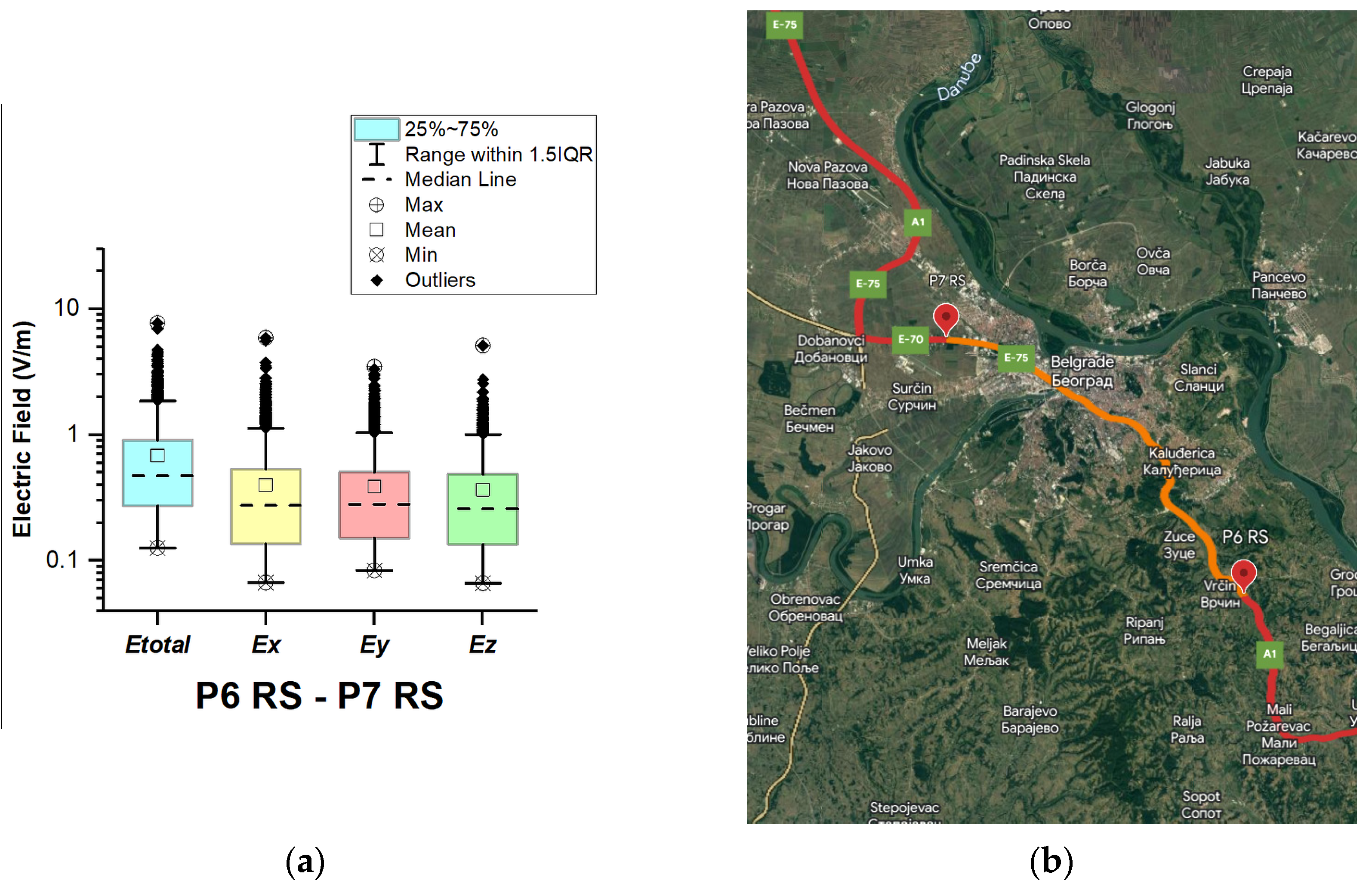
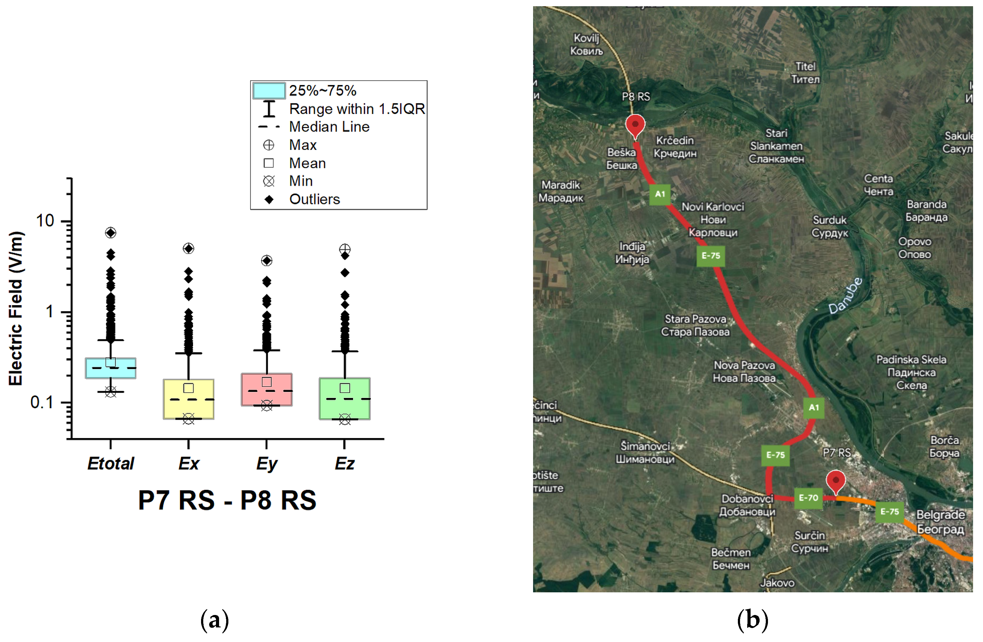
3.1.7. The Republic of Serbia
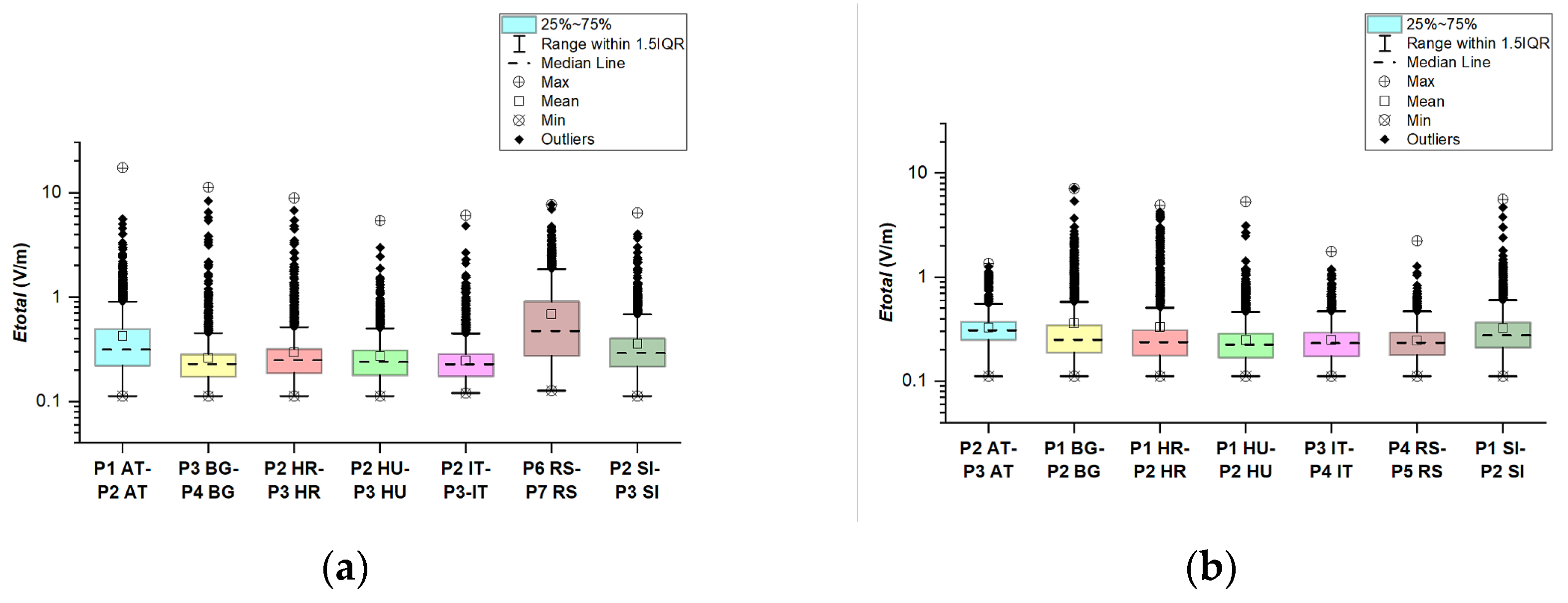
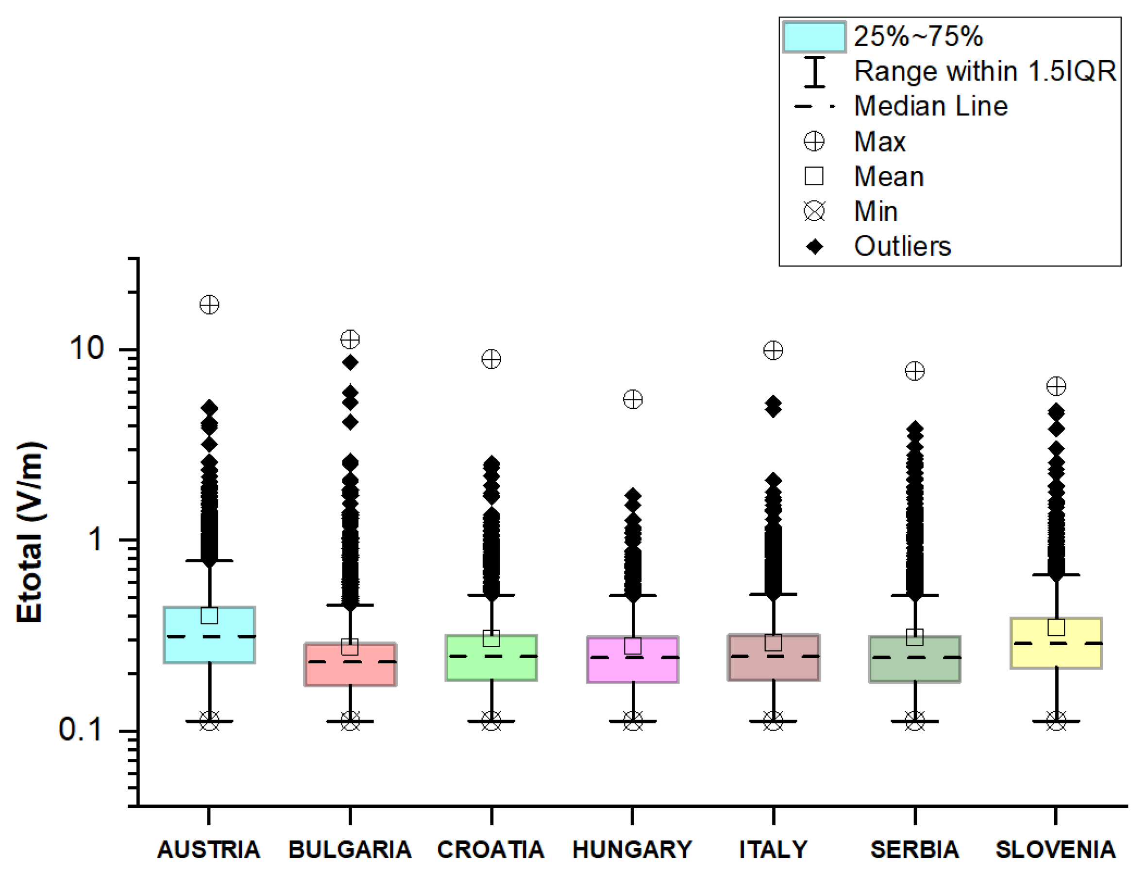
3.2. Comparison of Results between Different European Countries
4. Conclusions
Author Contributions
Funding
Institutional Review Board Statement
Informed Consent Statement
Data Availability Statement
Conflicts of Interest
References
- United Nations Publications. Sustainable Mobility and Smart Connectivity; United Nations: New York, NY, USA, 2021; pp. 45–96. [Google Scholar]
- Measuring Digital Development. Facts and Figures 2022. International Telecommunication Union. Telecommunication Development Sector. Available online: https://www.itu.int/itu-d/reports/statistics/facts-figures-2022/ (accessed on 30 November 2022).
- Atanasova, G.L.; Atanasov, B.N.; Atanasov, N.T. Fully Textile Dual-Band Logo Antenna for IoT Wearable Devices. Sensors 2022, 22, 4516. [Google Scholar] [CrossRef]
- Tognola, G.; Bonato, M.; Benini, N.; Aerts, S.; Gallucci, S.; Chiaramello, E.; Fiocchi, S.; Parazzini, M.; Masini, B.M.; Joseph, W.; et al. Survey of Exposure to RF Electromagnetic Fields in the Connected Car. IEEE Access 2022, 10, 47764–47781. [Google Scholar] [CrossRef]
- Tognola, G.; Masini, B.M.; Galluxxi, S.; Bonato, M.; Fiocchi, S.; Chiaramello, E.; Parazzini, M.; Ravazzani, P. Numerical Assessment of RF Human Exposure in Smart Mobility Communications. IEEE J. Electromagn. RF Microw. Med. Biol. 2021, 5, 100–107. [Google Scholar] [CrossRef]
- European Commission. Available online: https://commission.europa.eu/eu-regional-and-urban-development/topics/cities-and-urban-development/city-initiatives/smart-cities_en (accessed on 15 May 2023).
- Aerts, S.; Deprez, K.; Verloock, L.; Olsen, R.G.; Martens, L.; Tran, P.; Joseph, W. RF-EMF Exposure near 5G NR Small Cells. Sensors 2023, 23, 3145. [Google Scholar] [CrossRef] [PubMed]
- Iakovidis, S.; Apostolidis, C.; Manassas, A.; Samaras, T. Electromagnetic Fields Exposure Assessment in Europe Utilizing Publicly Available Data. Sensors 2022, 22, 8481. [Google Scholar] [CrossRef]
- Mulugeta, B.A.; Wang, S.; Ben Chikha, W.; Liu, J.; Roblin, C.; Wiart, J. Statistical Characterization and Modeling of Indoor RF-EMF Down-Link Exposure. Sensors 2023, 23, 3583. [Google Scholar] [CrossRef]
- Ramirez-Vazquez, R.; Gonzalez-Rubio, J.; Arribas, E.; Najera, A. Personal RF-EMF exposure from mobile phone base stations during temporary events. Environ. Res. 2019, 175, 266–273. [Google Scholar] [CrossRef]
- European Parliament. Available online: https://ehtrust.org/european-parliament-workshop-health-and-environmental-impacts-of-5g/ (accessed on 29 November 2020).
- Aguirre, E.; Arpon, J.; Azpilicueta, L.; Miguel-Bilbao, S.D.; Ramos-Gonzalez, M.V.; Falcone, F.J. Evaluation of electromagnetic dosimetry of wireless systems in complex indoor scenarios with human body interaction. Prog. Electromagn. Res. B 2012, 43, 189–209. [Google Scholar] [CrossRef] [Green Version]
- Chiaramello, E.; Bonato, M.; Fiocchi, S.; Tognola, G.; Parazzini, M.; Ravazzani, P.; Wiart, J. Radio frequency electromagnetic fields exposure assessment in indoor environments: A review. Int. J. Environ. Res. Public Health 2019, 16, 955. [Google Scholar] [CrossRef] [Green Version]
- Velghe, M.; Joseph, W.; Debouvere, S.; Aminzadeh, R.; Martens, L.; Thielens, A. Characterisation of spatial and temporal variability of RF-EMF exposure levels in urban environments in Flanders, Belgium. Environ. Res. 2019, 175, 351–366. [Google Scholar] [CrossRef]
- Sagar, S.; Adem, S.M.; Struchen, B.; Loughran, S.P.; Brunjes, M.E.; Arangua, L.; Dalvie, M.A.; Croft, R.J.; Jerrett, M.; Moskowitz, J.M.; et al. Comparison of radiofrequency electromagnetic field exposure levels in different everyday microenvironments in an international context. Environ. Int. 2018, 114, 297–306. [Google Scholar] [CrossRef] [PubMed]
- Bolte, J.F.; Maslanyj, M.; Addison, D.; Mee, T.; Kamer, J.; Colussi, L. Do car-mounted mobile measurements used for radio-frequency spectrum regulation have an application for exposure assessments in epidemiological studies? Environ. Int. 2016, 86, 75–83. [Google Scholar] [CrossRef] [PubMed]
- ICNIRP. Guidelines for Limiting Exposure to Electromagnetic Fields (100 kHz to 300 GHz). Available online: https://www.icnirp.org/en/activities/news/news-article/rf-guidelines-2020-published.html/ (accessed on 11 March 2020). [CrossRef]
- Jalilian, H.; Eeftens, M.; Ziaei, M.; Röösli, M. Public exposure to radiofrequency electromagnetic fields in everyday microenvironments: An updated systematic review for Europe. Environ. Res. 2019, 176, 108517. [Google Scholar] [CrossRef] [PubMed]
- Kapetanakis, T.N.; Ioannidou, M.P.; Baklezos, A.T.; Nikolopoulos, C.D.; Sergaki, E.S.; Konstantaras, A.J.; Vardiambasis, I.O. Assessment of Radiofrequency Exposure in the Vicinity of School Environments in Crete Island, South Greece. Appl. Sci. 2022, 12, 4701. [Google Scholar] [CrossRef]
- Da Silva, J.; de Sousa, V.A., Jr.; Rodrigues, M.E.C.; Pinheiro, F.S.R.; da Silva, G.S.; Mendonça, H.B.; de Silva, R.Q.; da Silva, J.V.L.; Galdino, F.E.S.; de Carvalho, V.F.C.; et al. Human Exposure to Non-Ionizing Radiation from Indoor Distributed Antenna System: Shopping Mall Measurement Analysis. Sensors 2023, 23, 4579. [Google Scholar] [CrossRef]
- Sagar, S.; Struchen, B.; Finta, V.; Eeftens, M.; Röösli, M. Use of portable exposimeters to monitor radiofrequency electromagnetic field exposure in the everyday environment. Environ. Res. 2016, 150, 289–298. [Google Scholar] [CrossRef]
- Celaya-Echarri, M.; Azpilicueta, L.; Karpowicz, J.; Ramos, V.; Lopez-Iturri, P.; Falcone, F. From 2G to 5G Spatial Modeling of Personal RF-EMF Exposure Within Urban Public Trams. IEEE Access 2020, 8, 100930–100947. [Google Scholar] [CrossRef]
- Bonato, M.; Tognola, G.; Benini, M.; Gallucci, S.; Chiaramello, E.; Fiocchi, S.; Parazzini, M. Assessment of SAR in Road-Users from 5G-V2X Vehicular Connectivity Based on Computational Simulations. Sensors 2022, 22, 6564. [Google Scholar] [CrossRef]
- Lu, R.; Zhang, L.; Ni, J.; Fang, Y. 5G Vehicle-to-Everything Services: Gearing Up for Security and Privacy. Proc. IEEE 2020, 108, 373–389. [Google Scholar] [CrossRef]
- Sewalkar, P.; Seitz, J. Vehicle-to-Pedestrian Communication for Vulnerable Road Users: Survey, Design Considerations, and Challenges. Sensors 2019, 19, 358. [Google Scholar] [CrossRef] [Green Version]
- Honda. Available online: https://www.roadsport.com/owners/manual/activating-your-hondas-built-in-wifi-hotspot-and-audio-controls.htm (accessed on 12 March 2021).
- GMC. Available online: https://www.gmc.com/connectivity-technology/wifi-hotspot (accessed on 4 October 2022).
- Lee, S.; Lee, J.; Yoon, S.; Choi, J. Relationship between electric field exposure and whole-body averaged SAR in automotive environments. In Proceedings of the 10th European Conference on Antennas and Propagation (EuCAP), Davos, Switzerland, 10–15 April 2016. [Google Scholar] [CrossRef]
- Low, L.; Zhang, H.; Rigelsford, J.; Langley, R. Computed field distributions within a passenger vehicle at 2.4 GHz. In Proceedings of the Loughborough Antennas & Propagation Conference, Loughborough, UK, 16–17 November 2009. [Google Scholar] [CrossRef]
- Anzaldi, G.; Silva, F.; Fernández, M.; Quílez, M.; Riu, P.J. Initial analysis of SAR from a cell phone inside a vehicle by numerical computation. IEEE Trans. Biomed. Eng. 2007, 54, 921–930. [Google Scholar] [CrossRef] [PubMed]
- Wang, S.; Mazloum, T.; Wiart, J. Prediction of RF-EMF Exposure by Outdoor Drive Test Measurements. Telecom 2022, 3, 396–406. [Google Scholar] [CrossRef]
- Onishi, T.; Esaki, K.; Tobita, K.; Ikuyo, M.; Taki, M.; Watanabe, S. Large-Area Monitoring of Radiofrequency Electromagnetic Field Exposure Levels from Mobile Phone Base Stations and Broadcast Transmission Towers by Car-Mounted Measurements around Tokyo. Electronics 2023, 12, 1835. [Google Scholar] [CrossRef]
- Eurostat. Available online: https://ec.europa.eu/eurostat/statistics-explained/index.php?title=Passenger_mobility_statistics#Mobility_data_for_thirteen_Member_States_with_different_characteristics (accessed on 11 November 2022).
- Bureau of Transportation Statistics. Available online: https://www.bts.gov/statistical-products/surveys/national-household-travel-survey-daily-travel-quick-facts (accessed on 31 May 2017).
- Eurostat. Available online: https://ec.europa.eu/eurostat/web/products-eurostat-news/-/edn-20200916-1 (accessed on 16 September 2020).
- Statista. Available online: https://www.statista.com/statistics/958135/vacation-travel-spending-of-europeans-by-country/ (accessed on 20 January 2012).
- LUMILOOP GmbH. Available online: https://lumiloop.de/products/lsprobe-laser-powered-e-field-probes/lsprobe-1-2/ (accessed on 9 February 2017).
- Panagiotakopoulos, T.; Kiouvrekis, Y.; Misthos, L.-M.; Kappas, C. RF-EMF Exposure Assessments in Greek Schools to Support Ubiquitous IoT-Based Monitoring in Smart Cities. IEEE Access 2023, 11, 7145–7156. [Google Scholar] [CrossRef]
- Zhou, Z.; Zhu, Q.; Liu, Y.; Zhang, Y.; Jia, Z.; Wu, G. Construction of Self-Assembly Based Tunable Absorber: Lightweight, Hydrophobic and Self-Cleaning Properties. Nano Micro Lett. 2023, 15, 137. [Google Scholar] [CrossRef] [PubMed]


| Parameter | |
|---|---|
| Measurement mode | 0 |
| Frequency range (GHz) | 0.03–8.2 |
| Sampling rate (kS/s) | 500 |
| Sample timing | continuous |
| Sensitivity (mV/m) | 60 |
| Country | Road Sector | Distance (km) | Total Distance (km) |
|---|---|---|---|
| Austria | P1 AT–P2 AT | 107.0 | 219.0 |
| P2 AT–P3 AT | 112.0 | ||
| Bulgaria | P1 BG–P2 BG | 44.1 | 304.4 |
| P2 BG–P3 BG | 84.3 | ||
| P3 BG–P4 BG | 179.0 | ||
| Croatia | P1 HR–P2 HR | 67.3 | 303.3 |
| P2 HR–P3 HR | 236.0 | ||
| Hungary | P1 HU–P2 HU | 52.6 | 160.5 |
| P2 HU–P3 HU | 58.7 | ||
| P3 HU–P4 HU | 49.2 | ||
| Italy | P1 IT–P2 IT | 8.3 | 377.4 |
| P2 IT–P3 IT | 100.0 | ||
| P3 IT–P4 IT | 69.7 | ||
| P4 IT–P5 IT | 53.4 | ||
| P5 IT–P1 Sl | 146.0 | ||
| Slovenia | P1 Sl–P2 Sl | 58.6 | 186.5 |
| P2 Sl–P3 Sl | 128.0 | ||
| Republic of Serbia | P1 RS–P2 RS | 28.8 | 391.9 |
| P2 RS–P3 RS | 125.0 | ||
| P3 RS–P4 RS | 36.9 | ||
| P4 RS–P5 RS | 69.8 | ||
| P5 RS–P6 RS | 50.3 | ||
| P6 RS –P7 RS | 32.4 | ||
| P7 RS–P8 RS | 48.7 |
| Country | Road Sector | N | Mean | Min | Median | Max |
|---|---|---|---|---|---|---|
| Austria | P1 AT–P2 AT | 28,762 | 0.420 | 0.111 | 0.313 | 17.395 |
| P2 AT–P3 AT | 14,684 | 0.326 | 0.111 | 0.308 | 1.353 | |
| Bulgaria | P1 BG–P2 BG | 7905 | 0.358 | 0.111 | 0.250 | 7.144 |
| P2 BG–P3 BG | 17,174 | 0.264 | 0.111 | 0.220 | 9.601 | |
| P3 BG–P4 BG | 34,404 | 0.261 | 0.111 | 0.226 | 11.332 | |
| Croatia | P1 HR–P2 HR | 8421 | 0.330 | 0.111 | 0.237 | 4.940 |
| P2 HR–P3 HR | 30,322 | 0.294 | 0.111 | 0.247 | 8.959 | |
| Hungary | P1 HU–P2 HU | 11,067 | 0.250 | 0.111 | 0.224 | 5.329 |
| P2 HU–P3 HU | 13,022 | 0.268 | 0.111 | 0.238 | 5.468 | |
| P3 HU–P4 HU | 9461 | 0.317 | 0.126 | 0.263 | 5.500 | |
| Italy | P1 IT–P2 IT | 5358 | 0.329 | 0.111 | 0.275 | 3.803 |
| P2 IT–P3 IT | 14,277 | 0.247 | 0.120 | 0.227 | 6.117 | |
| P3 IT–P4 IT | 6784 | 0.249 | 0.111 | 0.232 | 1.761 | |
| P4 IT–P5 IT | 18,241 | 0.289 | 0.111 | 0.247 | 7.209 | |
| P5 IT–P1 Sl | 18,550 | 0.318 | 0.111 | 0.255 | 9.941 | |
| Slovenia | P1 Sl–P2 Sl | 12,187 | 0.323 | 0.111 | 0.275 | 5.606 |
| P2 Sl–P3 Sl | 26,709 | 0.354 | 0.111 | 0.289 | 6.455 | |
| Republic of Serbia | P1 RS–P2 RS | 4944 | 0.223 | 0.111 | 0.215 | 3.121 |
| P2 RS–P3 RS | 10,073 | 0.270 | 0.120 | 0.231 | 3.519 | |
| P3 RS–P4 RS | 3452 | 0.251 | 0.126 | 0.234 | 3.935 | |
| P4 RS–P5 RS | 10,217 | 0.246 | 0.111 | 0.234 | 2.236 | |
| P5 RS–P6 RS | 7164 | 0.241 | 0.111 | 0.227 | 1.699 | |
| P6 RS–P7 RS | 5795 | 0.685 | 0.126 | 0.473 | 7.756 | |
| P7 RS–P8 RS | 6488 | 0.282 | 0.133 | 0.244 | 7.572 |
Disclaimer/Publisher’s Note: The statements, opinions and data contained in all publications are solely those of the individual author(s) and contributor(s) and not of MDPI and/or the editor(s). MDPI and/or the editor(s) disclaim responsibility for any injury to people or property resulting from any ideas, methods, instructions or products referred to in the content. |
© 2023 by the authors. Licensee MDPI, Basel, Switzerland. This article is an open access article distributed under the terms and conditions of the Creative Commons Attribution (CC BY) license (https://creativecommons.org/licenses/by/4.0/).
Share and Cite
Atanasova, G.L.; Atanasov, B.N.; Atanasov, N.T. Assessment of Electromagnetic Field Exposure on European Roads: A Comprehensive In Situ Measurement Campaign. Sensors 2023, 23, 6050. https://doi.org/10.3390/s23136050
Atanasova GL, Atanasov BN, Atanasov NT. Assessment of Electromagnetic Field Exposure on European Roads: A Comprehensive In Situ Measurement Campaign. Sensors. 2023; 23(13):6050. https://doi.org/10.3390/s23136050
Chicago/Turabian StyleAtanasova, Gabriela Lachezarova, Blagovest Nikolaev Atanasov, and Nikolay Todorov Atanasov. 2023. "Assessment of Electromagnetic Field Exposure on European Roads: A Comprehensive In Situ Measurement Campaign" Sensors 23, no. 13: 6050. https://doi.org/10.3390/s23136050