
Similarity-Driven Fine-Tuning Methods for Regularization Parameter Optimization in PET Image Reconstruction

Abstract
:1. Introduction
2. Methods
2.1. Penalized Likelihood Approach
2.2. Similarity-Driven Hyperparameter Tuning
2.3. Derivation of PL Reconstruction Algorithm
3. Results
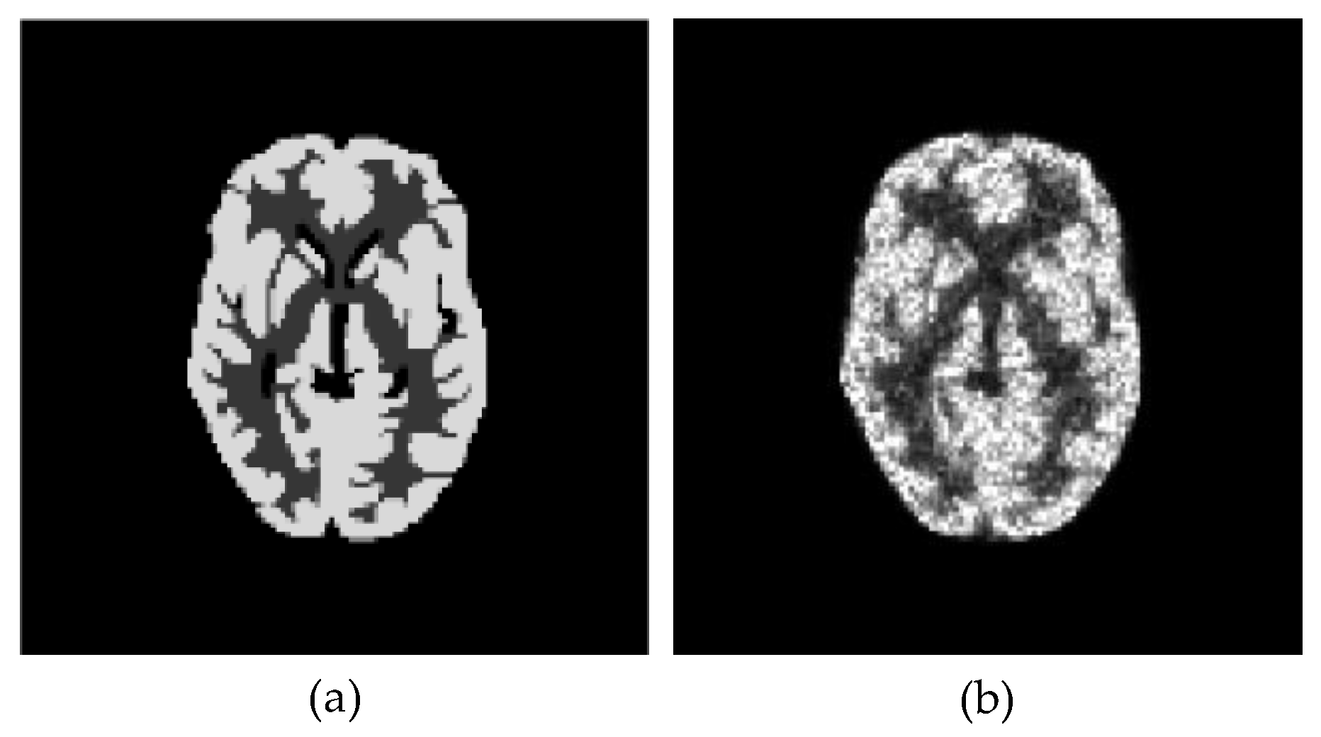
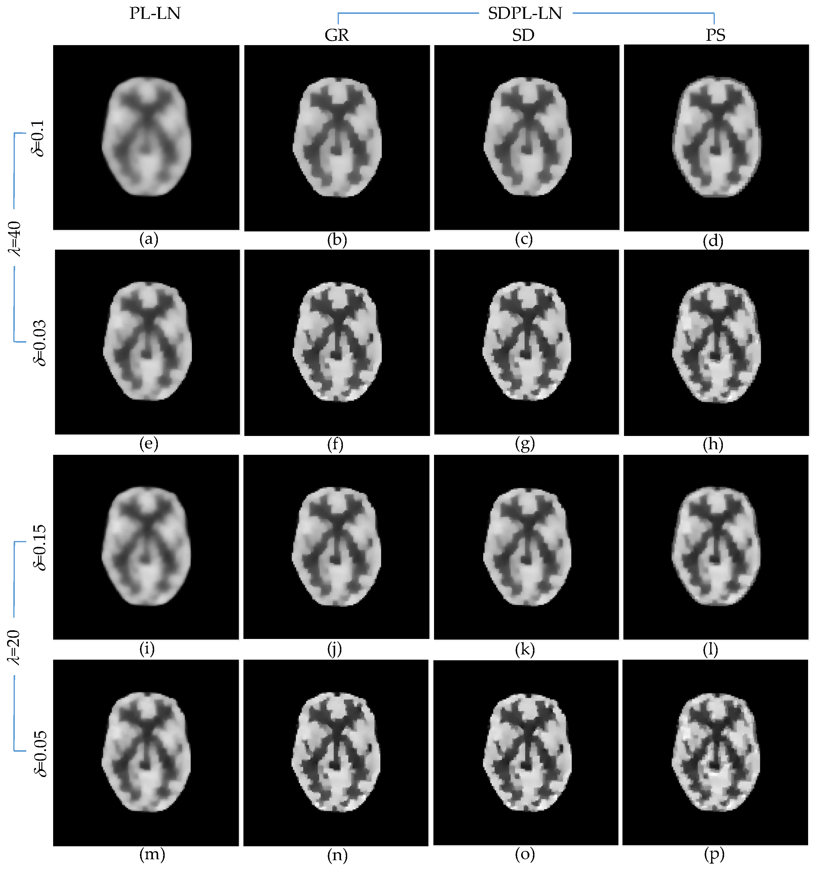
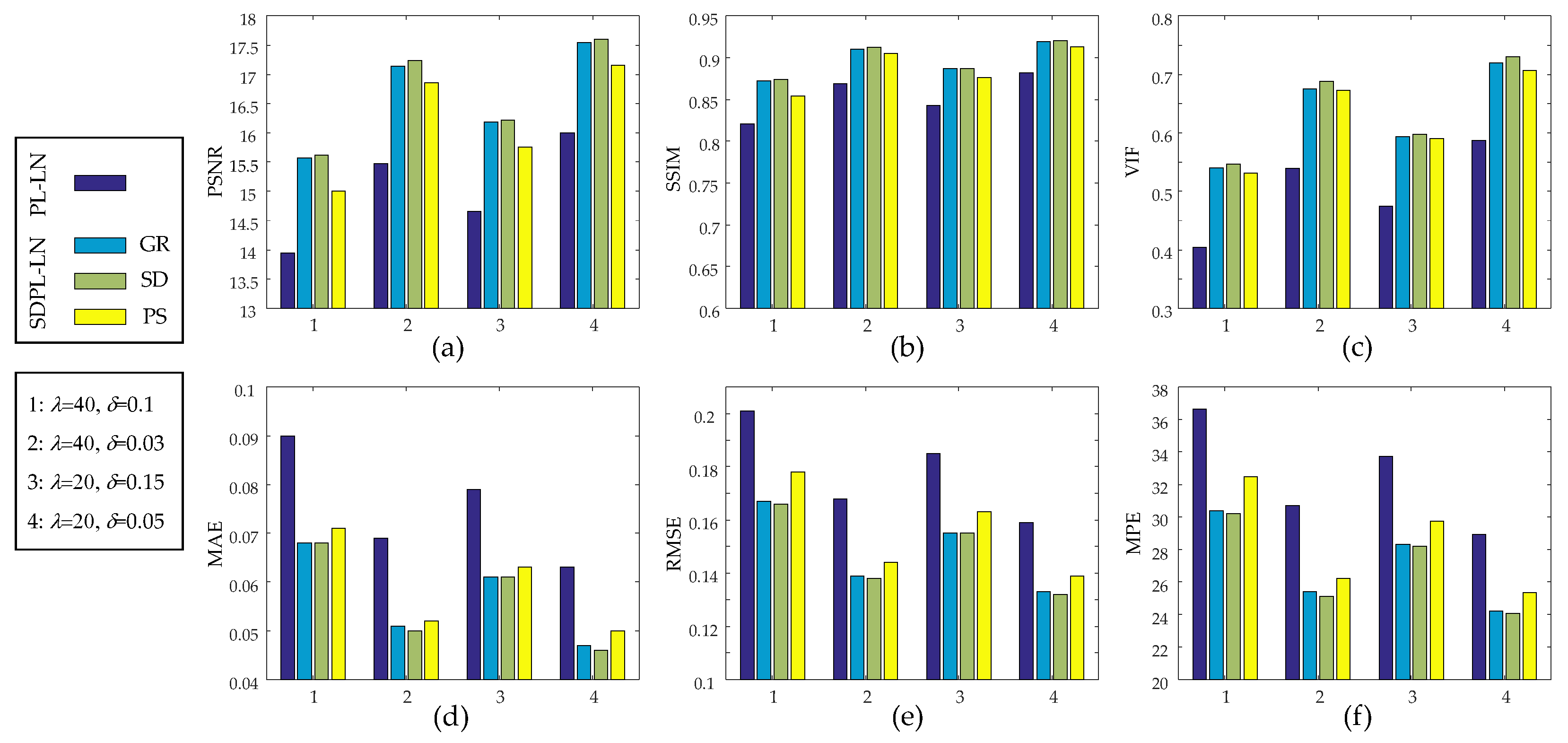
3.1. Numerical Studies Using Digital Phantom
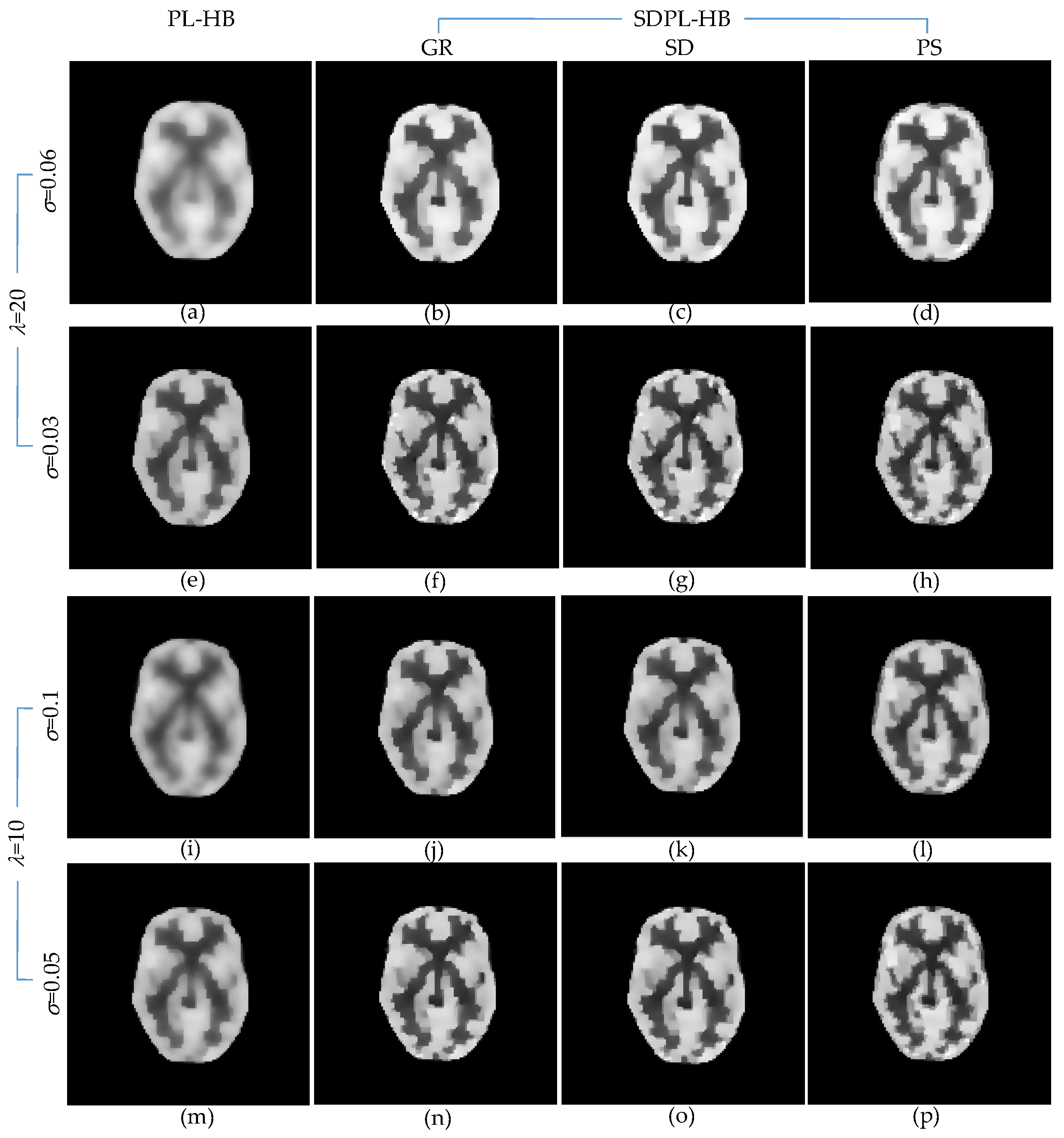
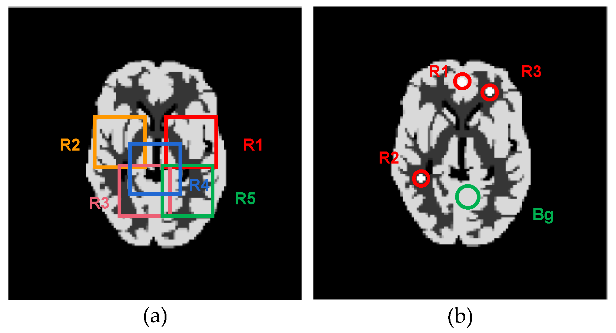
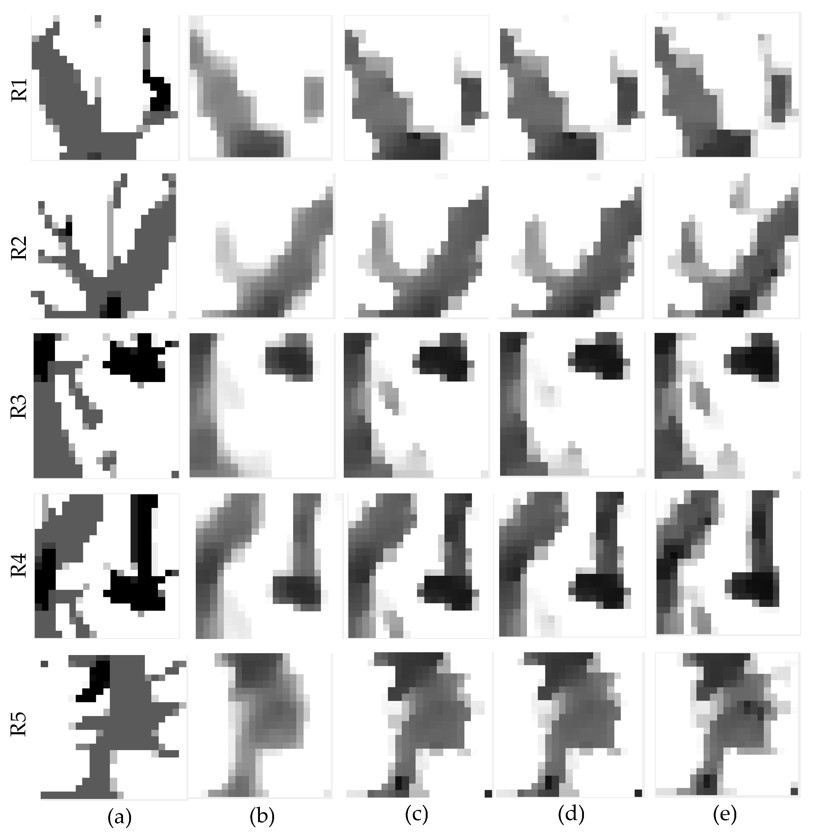
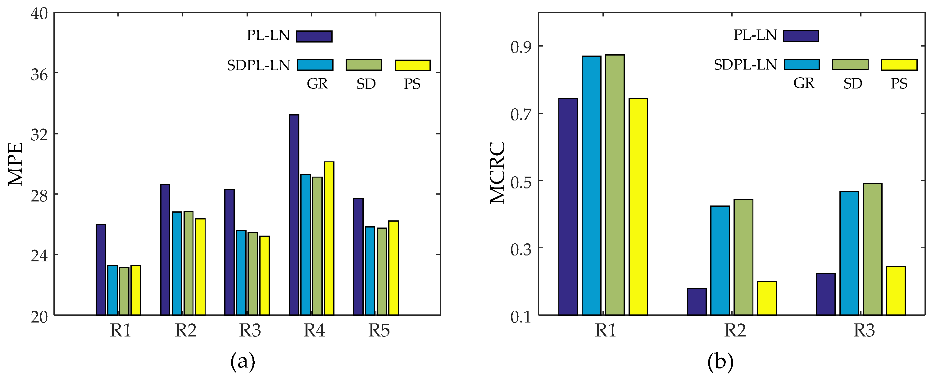
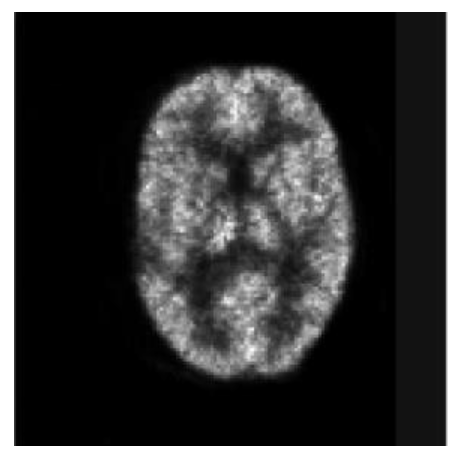
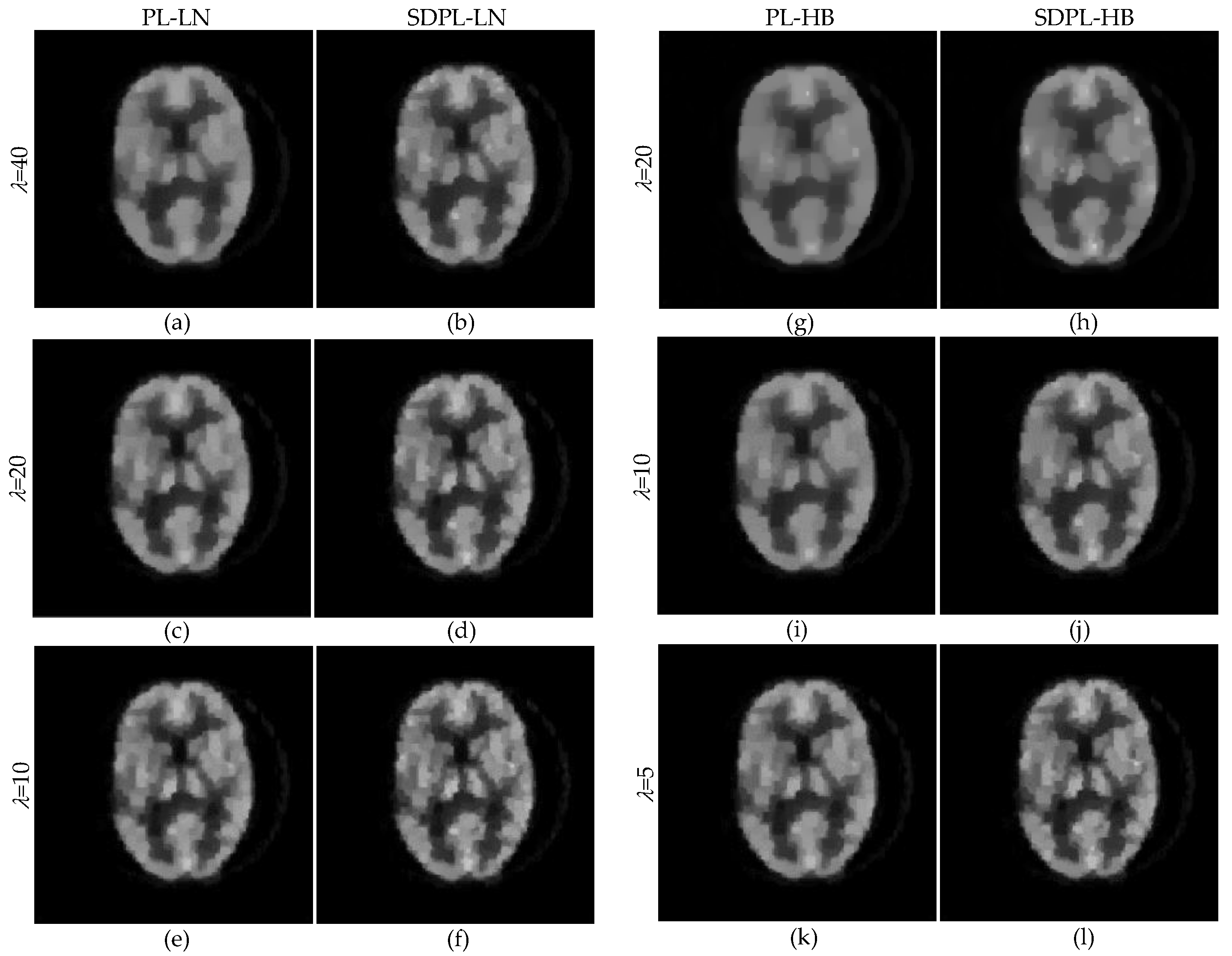
3.2. Qualitative Validation Using Physically Acquired Data
4. Summary and Conclusions
Author Contributions
Funding
Institutional Review Board Statement
Informed Consent Statement
Data Availability Statement
Conflicts of Interest
References
- Cherry, S.R.; Sorenson, J.A.; Phelps, M.E. Physics in Nuclear Medicine; Saunders: Philadelphia, PA, USA, 2012. [Google Scholar]
- Ollinger, J.H.; Fessler, J.A. Positron Emission Tomography. IEEE Signal Process. Mag. 1997, 14, 43–55. [Google Scholar] [CrossRef]
- Lewitt, R.M.; Matej, S. Overview of methods for image reconstruction from projections in emission computed tomography. Proc. IEEE 2003, 91, 1588–1611. [Google Scholar] [CrossRef]
- Tong, S.; Alessio, A.M.; Kinahan, P. Image reconstruction for PET/CT scanners: Past achievements and future challenges. Imaging Med. 2010, 2, 529–545. [Google Scholar] [CrossRef] [Green Version]
- Reader, A.J.; Zaidi, H. Advances in PET image reconstruction. PET Clin. 2007, 2, 173–190. [Google Scholar] [CrossRef]
- Qi, J.; Leahy, R.M. Iterative reconstruction techniques in emission computed tomography. Phys. Med. Biol. 2006, 51, 541–578. [Google Scholar] [CrossRef] [PubMed]
- Gong, K.; Berg, E.; Cherry, S.R.; Qi, J. Machine learning in PET: From photon detection to quantitative image reconstruction. Proc. IEEE 2019, 108, 51–68. [Google Scholar] [CrossRef]
- Reader, A.J.; Corda, G.; Mehranian, A.; da Costa-Luis, C.; Ellis, S.; Schnabel, J.A. Deep Learning for PET image reconstruction. IEEE Trans. Rad. Plasma Med. Sci. 2021, 5, 1–25. [Google Scholar] [CrossRef]
- Hashimoto, F.; Ote, K.; Onishi, Y. PET image reconstruction incorporating deep image prior and a forward projection model. IEEE Trans. Radiat. Plasma Med. Sci. 2022, 6, 841–846. [Google Scholar] [CrossRef]
- Kim, K.; Wu, D.; Gong, K.; Dutta, J.; Kim, J.H.; Son, Y.D.; Kim, H.K.; El Fakhri, G.; Li, Q. Penalized PET Reconstruction Using Deep Learning Prior and Local Linear Fitting. IEEE Trans. Med. Imaging 2018, 37, 1478–1487. [Google Scholar] [CrossRef]
- Hong, X.; Zan, Y.; Weng, F.; Tao, W.; Peng, Q.; Huang, Q. Enhancing the Image Quality via Transferred Deep Residual Learning of Coarse PET Sinograms. IEEE Trans. Med. Imaging 2018, 37, 2322–2332. [Google Scholar] [CrossRef]
- Kang, E.; Min, J.; Ye, J.C. A deep convolutional neural network using directional wavelets for low-dose X-ray CT reconstruction. Med. Phys. 2017, 44, e360–e375. [Google Scholar] [CrossRef] [PubMed] [Green Version]
- Pain, C.D.; Egan, G.F.; Chen, Z. Deep learning-based image reconstruction and post-processing methods in positron emission tomography for low-dose imaging and resolution enhancement. Eur. J. Nucl. Med. Mol. Imaging 2022, 49, 3098–3118. [Google Scholar] [CrossRef] [PubMed]
- Mehranian, A.; Reader, J. Model-based deep learning PET image reconstruction using forward-backward splitting expectation-maximization. IEEE Trans. Rdiat. Plasma Med. Sci. 2020, 5, 54–64. [Google Scholar] [CrossRef]
- Adler, J.; Öktem, O. Learned primal-dual reconstruction. IEEE Trans. Med. Imaging 2018, 37, 1322–1332. [Google Scholar] [CrossRef] [PubMed] [Green Version]
- Hansen, P.C. Analysis of discrete ill-posed problems by means of the L-curve. SIAM Rev. 1992, 34, 561–580. [Google Scholar] [CrossRef]
- Golub, G.H.; Heath, M.; Wahba, G. Generalized cross-validation as a method for choosing a good ridge parameter. Technometrics 1979, 21, 215–223. [Google Scholar] [CrossRef]
- Ramani, S.; Liu, Z.; Nielsen, J.-F.; Fessler, J.A. Regularization parameter selection for nonlinear iterative image restoration and MRI reconstruction using GCV and sure-based methods. IEEE Trans. Image Process. 2012, 21, 3659–3672. [Google Scholar] [CrossRef] [Green Version]
- Zhu, X.; Milanfar, P. Automatic parameter selection for denoising algorithms using a no-reference measure of image content. IEEE Trans. Image Process. 2010, 19, 3116–3132. [Google Scholar]
- Liang, H.; Weller, D.S. Comparison-based image quality assessment for selecting image restoration parameters. IEEE Trans Image Process. 2016, 25, 5118–5130. [Google Scholar] [CrossRef] [Green Version]
- Shen, C.; Gonzalez, Y.; Chen, L.; Jiang, S.B.; Jia, X. Intelligent parameter tuning in optimization-based iterative CT reconstruction via deep reinforcement learning. IEEE Trans. Med. Imaging 2018, 37, 1430–1439. [Google Scholar] [CrossRef]
- Xu, J.; Noo, F. Patient-specific hyperparameter learning for optimization-based CT image reconstruction. Phys. Med. Biol. 2021, 66, 19. [Google Scholar] [CrossRef] [PubMed]
- Lee, J.; Lee, S.-J. Smoothing-parameter tuning for regularized PET image reconstruction using deep learning. In Proceedings of the SPIE 12463, Medical Imaging 2023: Physics of Medical Imaging, San Diego, CA, USA, 19–23 February 2023. [Google Scholar]
- Lee, S.-J. Performance comparison of convex-nonquadratic priors for Bayesian tomographic reconstruction. J. Electron. Imaging 2000, 9, 242–250. [Google Scholar] [CrossRef]
- Buades, A.; Coll, B.; Morel, J.M. A review of image denoising algorithms, with a new one. Multiscale Model. Simul. 2005, 4, 490–530. [Google Scholar] [CrossRef]
- Deledalle, C.-A.; Denis, L.; Tupin, F. Iterative weighted maximum likelihood denoising with probabilistic patch-based weights. IEEE Trans. Image Process. 2009, 18, 2661–2672. [Google Scholar] [CrossRef] [PubMed] [Green Version]
- Sharifymoghaddam, M.; Beheshti, S.; Elahi, P.; Hashemi, M. Similarity validation based nonlocal means image denoising. IEEE Sig. Process. Lett. 2015, 22, 2185–2188. [Google Scholar] [CrossRef]
- Zhang, X.; Feng, X.; Wang, W. Two-direction nonlocal model for image denoising. IEEE Trans. Image Process. 2013, 22, 408–412. [Google Scholar] [CrossRef]
- Leal, N.; Zurek, E.; Leal, E. Non-local SVD denoising of MRI based on sparse representations. Sensors 2020, 20, 1536. [Google Scholar] [CrossRef] [Green Version]
- Nguyen, V.-G.; Lee, S.-J. Incorporating anatomical side information into PET reconstruction using nonlocal regularization. IEEE Trans. Image Process. 2013, 22, 3961–3973. [Google Scholar] [CrossRef]
- Wang, G.; Qi, J. Penalized likelihood PET image reconstruction using patch-based edge-preserving regularization. IEEE Trans. Med. Imaging 2012, 31, 2194–2204. [Google Scholar] [CrossRef] [Green Version]
- Tahaei, M.S.; Reader, A.J. Patch-based image reconstruction for PET using prior-image derived dictionaries. Phys. Med. Biol. 2016, 61, 6833–6855. [Google Scholar] [CrossRef]
- Xie, N.; Chen, Y.; Liu, H. 3D tensor based nonlocal low rank approximation in dynamic PET reconstruction. Sensors 2019, 19, 5299. [Google Scholar] [CrossRef] [PubMed] [Green Version]
- Ren, X.; Lee, S.-J. Penalized-likelihood PET image reconstruction using similarity-driven median regularization. Tomography 2022, 8, 158–174. [Google Scholar] [CrossRef] [PubMed]
- Lange, K. Convergence of EM image reconstruction algorithms with Gibbs smoothing. IEEE Trans. Med. Imaging 1990, 9, 439–446. [Google Scholar] [CrossRef] [PubMed]
- Huber, P.J. Robust Statistics; John Wiley & Sons: New York, NY, USA, 1981. [Google Scholar]
- Li, S.Z. Close-form solution and parameter selection for convex minimization-based edge-preserving smoothing. IEEE Trans. Pattern Anal. Mach. Intell. 1998, 20, 916–932. [Google Scholar] [CrossRef]
- Hsiao, I.-T.; Rangarajan, A.; Gindi, G. An accelerated convergent ordered subset algorithm for emission tomography. Phys. Med. Biol. 2004, 49, 2145–2156. [Google Scholar] [CrossRef]
- Hudson, H.M.; Larkin, R.S. Accelerated image reconstruction using ordered subsets of projection data. IEEE Trans. Med. Imaging 1994, 13, 601–609. [Google Scholar] [CrossRef] [Green Version]
- Vardi, A.; Shepp, L.A.; Kaufman, L. A statistical model for positron emission tomography. J. R. Stat. Soc. 1985, 80, 8–37. [Google Scholar] [CrossRef]
- Erdoğan, H.; Fessler, J.A. Ordered subsets algorithms for transmission tomography. Phys. Med. Biol. 1999, 44, 2835–2851. [Google Scholar] [CrossRef]
- Ahn, S.; Fessler, J.A. Globally convergent image reconstruction for emission tomography using relaxed ordered subsets algorithms. IEEE Trans. Med. Imaging 2003, 22, 613–626. [Google Scholar] [CrossRef] [Green Version]
- Erdoğan, H.; Fessler, J.A. Monotonic algorithms for transmission tomography. IEEE Trans. Med. Imaging 1999, 18, 801–814. [Google Scholar] [CrossRef] [Green Version]
- De Pierro, A.R. A modified expectation maximization algorithm for penalized likelihood estimation in emission tomography. IEEE Trans. Med. Imaging 1995, 14, 132–137. [Google Scholar] [CrossRef] [PubMed]
- De Pierro, A.R. On the convergence of an EM-type algorithm for penalized likelihood estimation in emission tomography. IEEE Trans. Med. Imaging 1995, 14, 762–765. [Google Scholar] [CrossRef] [PubMed]
- Seshadrinathan, K.; Pappas, T.N.; Safranek, R.J.; Chen, J.; Wang, Z.; Sheikh, H.R.; Bovik, A.C. Image quality assessment. In The Essential Guide to Image Processing, 2nd ed.; Bovik. A, Ed.; Academic Press: Burlington, MA, USA, 2009; pp. 535–595. [Google Scholar]
- Wang, Z.; Bovik, A.C.; Sheikh, H.R.; Simoncelli, E.P. Image quality assessment: From error visibility to structural similarity. IEEE Trans. Image Process. 2004, 13, 600–612. [Google Scholar] [CrossRef] [PubMed] [Green Version]
- Sheikh, H.R.; Bovik, A.C. Image information and visual quality. IEEE Trans. Image Process. 2006, 15, 430–444. [Google Scholar] [CrossRef]
- Willmott, C.J.; Matsuura, K. Advantages of the mean absolute error (MAE) over the root mean square error (RMSE) in assessing average model performance. Clim. Res. 2005, 30, 79–82. [Google Scholar] [CrossRef]
- Panin, V.Y.; Zeng, G.L.; Gullberg, G.T. Total variation regulated EM algorithm. IEEE Trans. Nucl. Sci. 1999, 46, 2202–2210. [Google Scholar] [CrossRef]
- Burger, M.; Muller, J.; Papoutsellis, E.; Schonlieb, C.B. Total variation regularization in measurement and image space for PET reconstruction. Inv. Probl. 2014, 30, 105003. [Google Scholar] [CrossRef]
- Yu, H.; Chen, Z.; Zhang, H.; Loong Wong, K.K.; Chen, Y.; Liu, H. Reconstruction for 3D PET based on total variation constrained direct fourier method. PLoS ONE 2015, 10, 0138483. [Google Scholar] [CrossRef]
- Tang, J.; Yang, B.; Wang, Y.; Ying, L. Sparsity-constrained PET image reconstruction with learned dictionaries. Phys. Med. Biol. 2016, 61, 6347–6368. [Google Scholar] [CrossRef]
- Xie, N.; Gong, K.; Guo, N.; Qin, Z.; Wu, Z.; Liu, H.; Li, Q. Penalized-likelihood PET image reconstruction using 3D structural convolutional sparse coding. IEEE Trans. Biomed. Eng. 2022, 69, 4–14. [Google Scholar] [CrossRef]
- Ren, X.; Lee, S.-J. Joint sparse coding-based super-resolution PET image reconstruction. In Proceedings of the IEEE Nuclear Science Symposium and Medical Imaging Conference, Boston, MA, USA, 31 October–7 November 2020. [Google Scholar]
- Chen, S.; Liu, H.; Hu, Z.; Zhang, H.; Shi, P.; Chen, Y. Simultaneous reconstruction and segmentation of dynamic PET via low-rank and sparse matrix decomposition. IEEE Trans. Biomed. Eng. 2015, 62, 1784–1795. [Google Scholar] [CrossRef] [PubMed]


| IQA Metrics | PL-LN | SDPL-LN | |||
|---|---|---|---|---|---|
| GR | SD | PS | |||
| = 40 = 0.1 | PSNR(dB) | 13.943 | 15.569 | 15.621 | 14.999 |
| SSIM | 0.821 | 0.872 | 0.874 | 0.854 | |
| VIF | 0.404 | 0.540 | 0.547 | 0.531 | |
| MAE | 0.090 | 0.068 | 0.068 | 0.071 | |
| RMSE | 0.201 | 0.167 | 0.166 | 0.178 | |
| MPE | 36.651 | 30.396 | 30.216 | 32.459 | |
| = 40 = 0.03 | PSNR(dB) | 15.475 | 17.133 | 17.232 | 16.856 |
| SSIM | 0.869 | 0.910 | 0.912 | 0.905 | |
| VIF | 0.539 | 0.675 | 0.688 | 0.672 | |
| MAE | 0.069 | 0.051 | 0.050 | 0.052 | |
| RMSE | 0.168 | 0.139 | 0.138 | 0.144 | |
| MPE | 30.728 | 25.387 | 25.101 | 26.210 | |
| = 20 = 0.15 | PSNR(dB) | 14.659 | 16.186 | 16.222 | 15.756 |
| SSIM | 0.843 | 0.887 | 0.887 | 0.876 | |
| VIF | 0.474 | 0.593 | 0.598 | 0.590 | |
| MAE | 0.079 | 0.061 | 0.061 | 0.063 | |
| RMSE | 0.185 | 0.155 | 0.155 | 0.163 | |
| MPE | 33.754 | 28.311 | 28.194 | 29.748 | |
| = 20 = 0.05 | PSNR(dB) | 16.001 | 17.543 | 17.601 | 17.151 |
| SSIM | 0.882 | 0.919 | 0.920 | 0.913 | |
| VIF | 0.587 | 0.720 | 0.730 | 0.706 | |
| MAE | 0.063 | 0.047 | 0.046 | 0.050 | |
| RMSE | 0.159 | 0.133 | 0.132 | 0.139 | |
| MPE | 28.922 | 24.217 | 24.056 | 25.335 | |
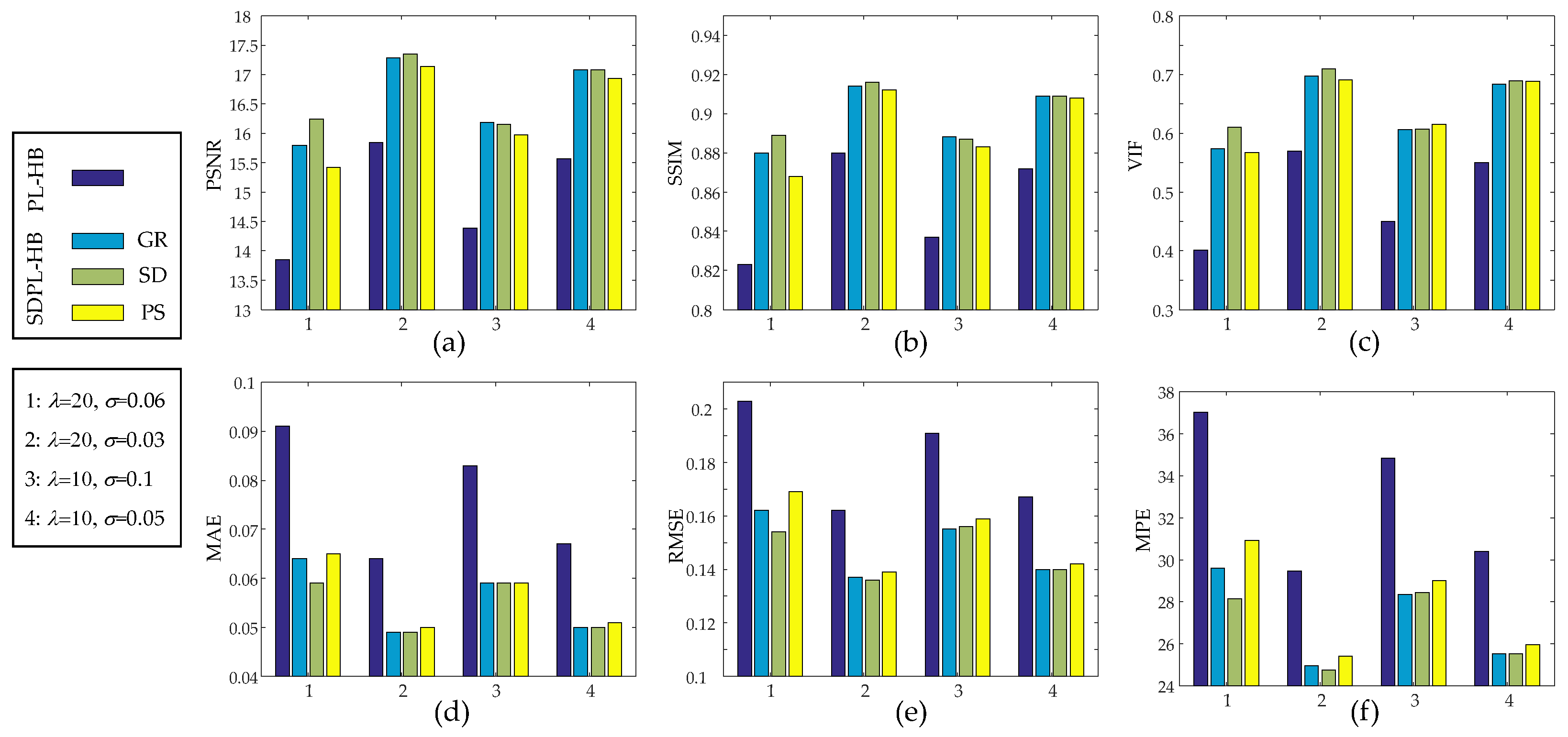
| IQA Metrics | PL-HB | SDPL-HB | |||
|---|---|---|---|---|---|
| GR | SD | PS | |||
| λ = 20 σ = 0.06 | PSNR(dB) | 13.857 | 15.798 | 16.239 | 15.421 |
| MSSIM | 0.823 | 0.880 | 0.889 | 0.868 | |
| VIF | 0.401 | 0.574 | 0.611 | 0.567 | |
| MAE | 0.091 | 0.064 | 0.059 | 0.065 | |
| RMSE | 0.203 | 0.162 | 0.154 | 0.169 | |
| MPE | 37.018 | 29.605 | 28.142 | 30.920 | |
| λ = 20 σ = 0.03 | PSNR(dB) | 15.838 | 17.277 | 17.353 | 17.134 |
| SSIM | 0.880 | 0.914 | 0.916 | 0.912 | |
| VIF | 0.569 | 0.697 | 0.710 | 0.691 | |
| MAE | 0.064 | 0.049 | 0.049 | 0.050 | |
| RMSE | 0.162 | 0.137 | 0.136 | 0.139 | |
| MPE | 29.469 | 24.971 | 24.755 | 25.386 | |
| λ = 10 σ = 0.1 | PSNR(dB) | 14.387 | 16.176 | 16.149 | 15.974 |
| SSIM | 0.837 | 0.888 | 0.887 | 0.883 | |
| VIF | 0.450 | 0.606 | 0.607 | 0.615 | |
| MAE | 0.083 | 0.059 | 0.059 | 0.059 | |
| RMSE | 0.191 | 0.155 | 0.156 | 0.159 | |
| MPE | 34.826 | 28.346 | 28.434 | 29.011 | |
| λ = 10 σ = 0.05 | PSNR(dB) | 15.564 | 17.086 | 17.086 | 16.938 |
| SSIM | 0.872 | 0.909 | 0.909 | 0.908 | |
| VIF | 0.550 | 0.684 | 0.689 | 0.688 | |
| MAE | 0.067 | 0.050 | 0.050 | 0.051 | |
| RMSE | 0.167 | 0.140 | 0.140 | 0.142 | |
| MPE | 30.412 | 25.526 | 25.527 | 25.963 | |
Disclaimer/Publisher’s Note: The statements, opinions and data contained in all publications are solely those of the individual author(s) and contributor(s) and not of MDPI and/or the editor(s). MDPI and/or the editor(s) disclaim responsibility for any injury to people or property resulting from any ideas, methods, instructions or products referred to in the content. |
© 2023 by the authors. Licensee MDPI, Basel, Switzerland. This article is an open access article distributed under the terms and conditions of the Creative Commons Attribution (CC BY) license (https://creativecommons.org/licenses/by/4.0/).
Share and Cite
Zhu, W.; Lee, S.-J. Similarity-Driven Fine-Tuning Methods for Regularization Parameter Optimization in PET Image Reconstruction. Sensors 2023, 23, 5783. https://doi.org/10.3390/s23135783
Zhu W, Lee S-J. Similarity-Driven Fine-Tuning Methods for Regularization Parameter Optimization in PET Image Reconstruction. Sensors. 2023; 23(13):5783. https://doi.org/10.3390/s23135783
Chicago/Turabian StyleZhu, Wen, and Soo-Jin Lee. 2023. "Similarity-Driven Fine-Tuning Methods for Regularization Parameter Optimization in PET Image Reconstruction" Sensors 23, no. 13: 5783. https://doi.org/10.3390/s23135783