
Growth Monitoring and Yield Estimation of Maize Plant Using Unmanned Aerial Vehicle (UAV) in a Hilly Region


Abstract
:1. Introduction
2. Materials and Methods
- Study Area
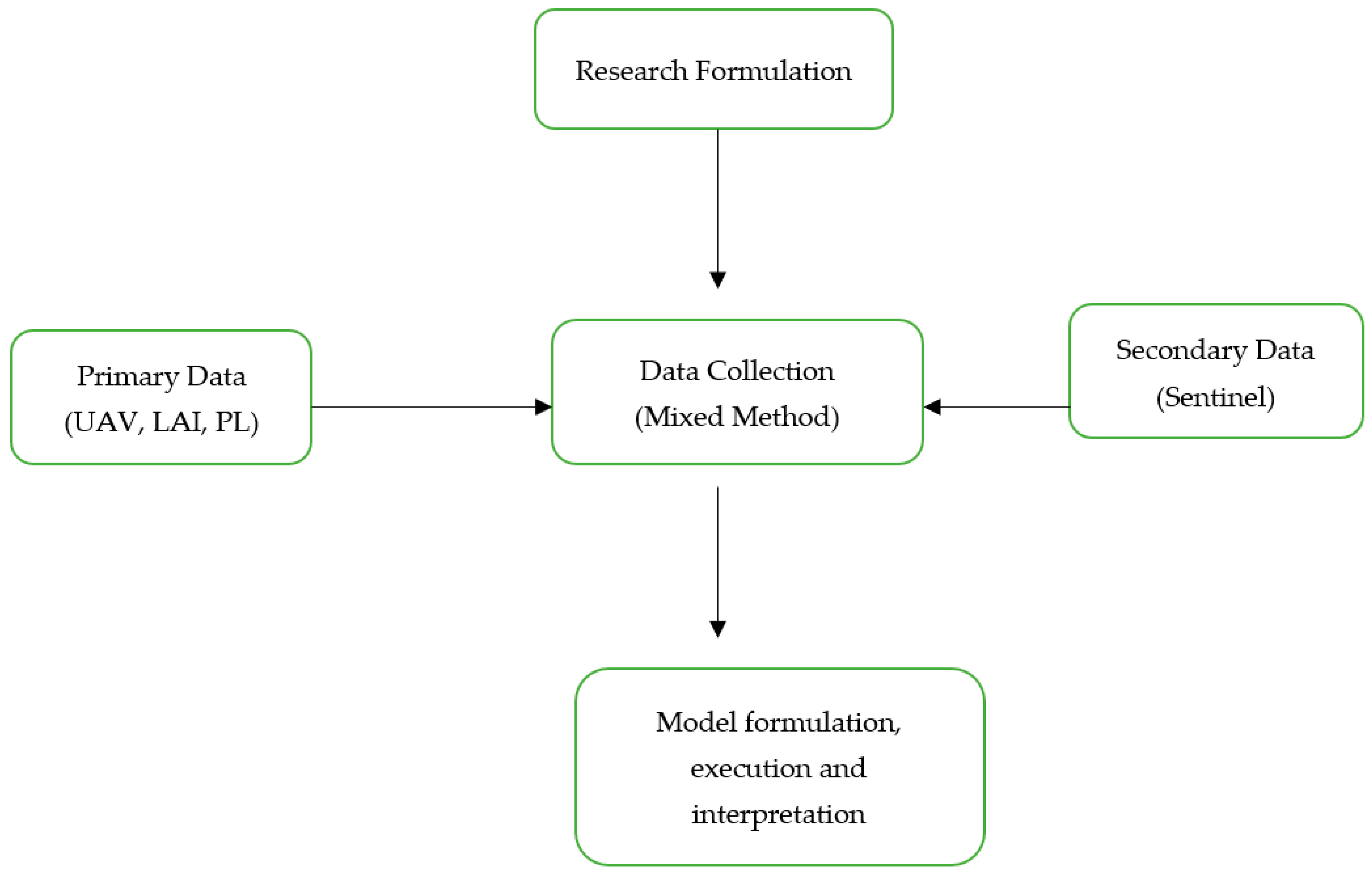
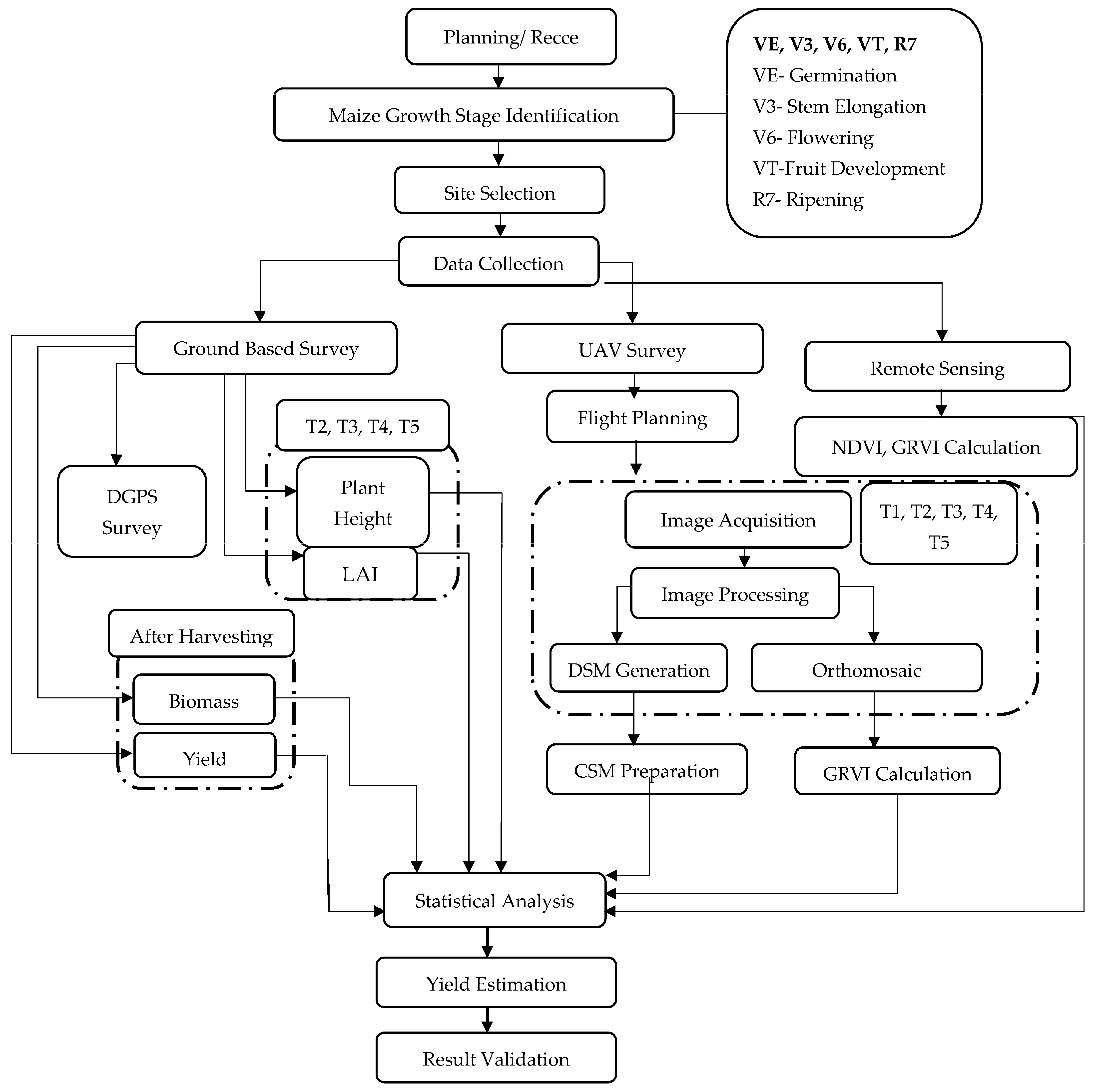
- Research Design
3. Results
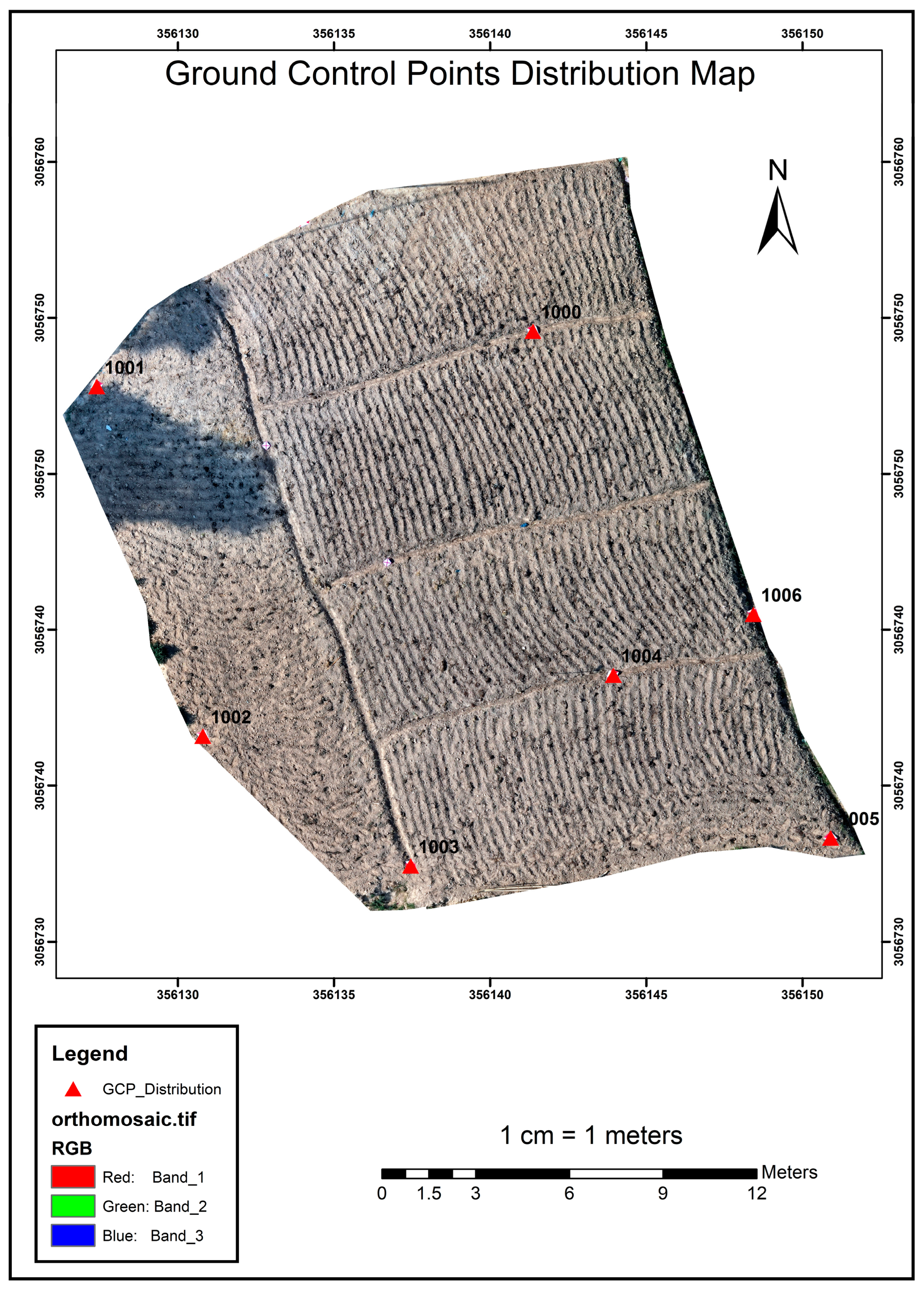
3.1. DGPS Survey Result
3.2. Growth Monitoring through Leaf Area Index
3.3. Growth Monitoring through Crop Surface Model
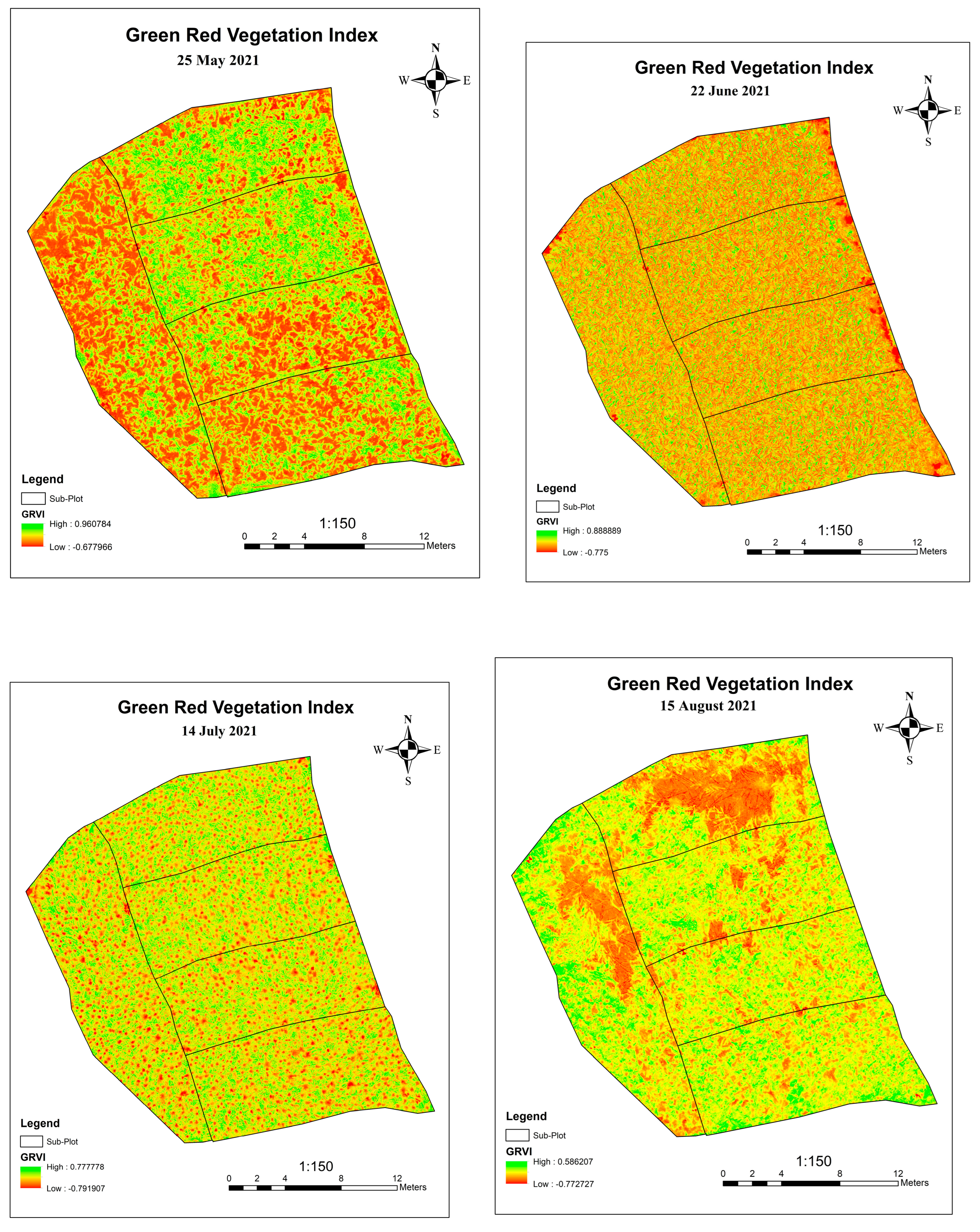
3.4. Growth Monitoring through Green–Red Vegetation Index
3.5. Relation between Crop Canopy Parameters
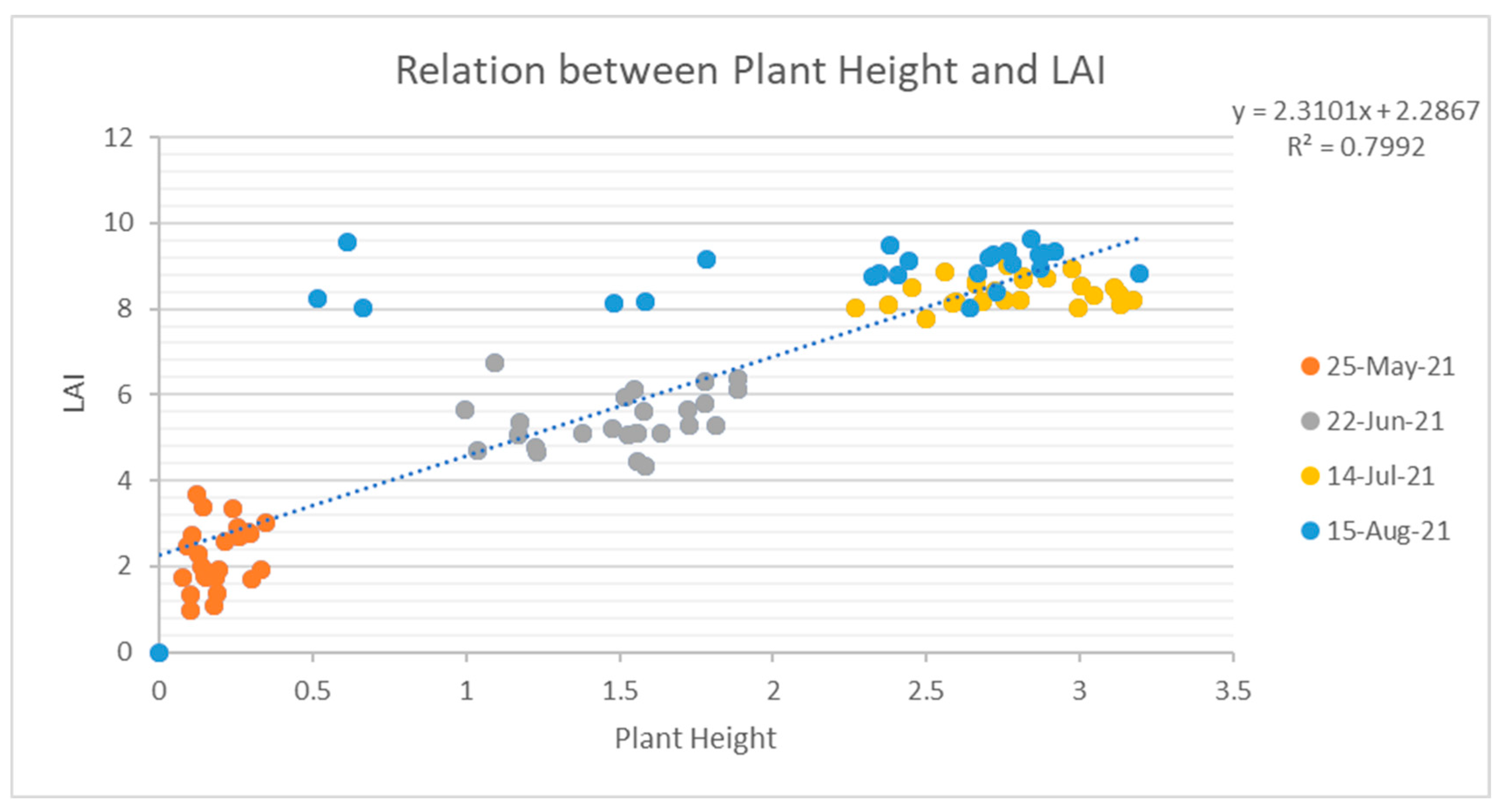
3.5.1. Relation between Plant Height and Leaf Area Index
3.5.2. Relation between GRVI and NDVI
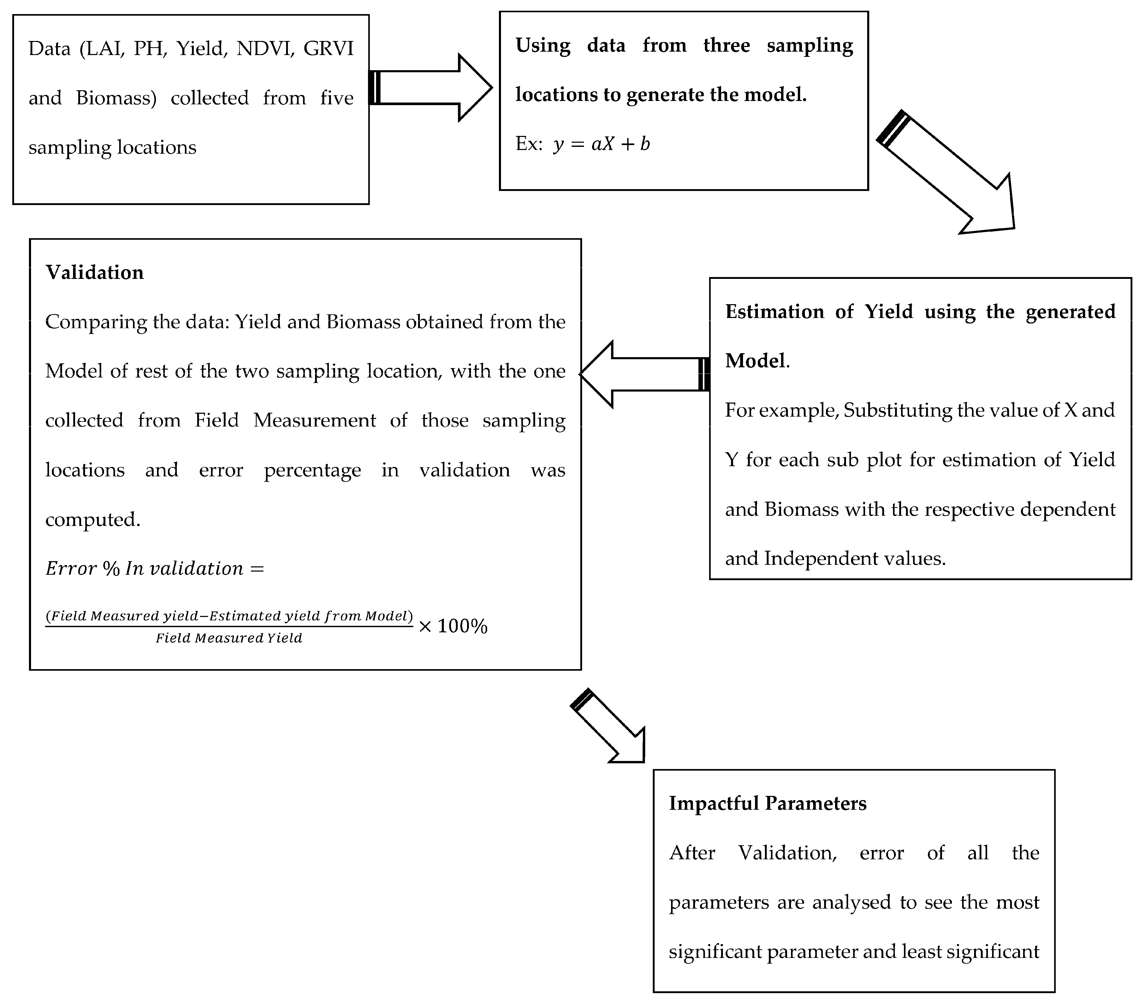
3.6. Model Generation, Estimation and Validation
3.6.1. Relation between Yield and Plant Height
3.6.2. Relation between Yield and Leaf Area Index
3.6.3. Relation between Yield and Green–Red Vegetation Index
3.6.4. Relation between Yield and Biomass
3.6.5. Relation between Yield and NDVI
3.6.6. Relation between Yield and Satellite-Based GRVI
3.6.7. Estimation of Yield from Plant Height
3.6.8. Estimation of Yield from Leaf Area Index (LAI)
3.6.9. Estimation of Yield from Green–Red Vegetation Index (GRVI)
3.6.10. Estimation of Yield from Biomass
3.6.11. Estimation of Yield from Normalized Difference Vegetation Index (NDVI)
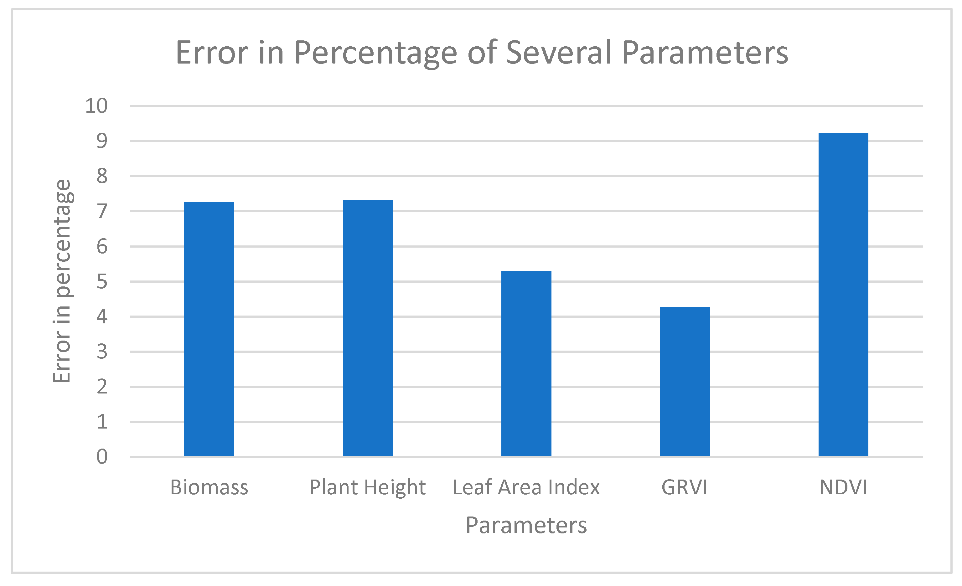
3.6.12. Analysis of Error to Select the Parameters
4. Discussion
Multiple Linear Regression Analysis
5. Conclusions
- GRVI is the most important parameter for estimating maize yield.
- Satellite-based NDVI is less important than UAV-based GRVI due to its lower spatial resolution and cloud cover.
- Future research should focus on incorporating higher-resolution NDVI data, genomic information, management practices, and environmental data into yield estimation models.
Author Contributions
Funding
Institutional Review Board Statement
Informed Consent Statement
Data Availability Statement
Acknowledgments
Conflicts of Interest
References
- World Bank. Food Security|Rising Food Insecurity in 2023. Available online: https://www.worldbank.org/en/topic/agriculture/brief/food-security-update (accessed on 23 March 2023).
- Ayim, C.; Kassahun, A.; Addison, C.; Tekinerdogan, B. Adoption of ICT innovations in the agriculture sector in Africa: A review of the literature. Agric. Food Secur. 2022, 11, 22. [Google Scholar] [CrossRef]
- National Academy of Sciences; National Academy of Engineering; Institute of Medicine. Population Summit of the World’s Scientific Academies; National Academies Press: Washington, DC, USA, 1993. [Google Scholar] [CrossRef]
- Radoglou-Grammatikis, P.; Sarigiannidis, P.; Lagkas, T.; Moscholios, I. A compilation of UAV applications for precision agriculture. Comput. Netw. 2020, 172, 107148. [Google Scholar] [CrossRef]
- Fertilizer Technology—An Overview|ScienceDirect Topics. Available online: https://www.sciencedirect.com/topics/agricultural-and-biological-sciences/fertilizer-technology (accessed on 25 March 2023).
- Liu, Y.; Bachofen, C.; Wittwer, R.; Silva Duarte, G.; Sun, Q.; Klaus, V.H.; Buchmann, N. Using PhenoCams to track crop phenology and explain the effects of different cropping systems on yield. Agric. Syst. 2022, 195, 103306. [Google Scholar] [CrossRef]
- Biomass—An Overview|ScienceDirect Topics. Available online: https://www.sciencedirect.com/topics/agricultural-and-biological-sciences/biomass (accessed on 24 March 2023).
- Assessing Carbon Stocks and Modelling Win-Win Scenarios of Carbon Sequestration though Land-Use Changes. Available online: https://www.fao.org/3/y5490e/y5490e07.htm (accessed on 24 March 2023).
- Khan, I.; Akhtar, M.W. Bioenergy Production from Plant Biomass: Bioethanol from Concept to Reality. Nat. Prec. 2011, 1. [Google Scholar] [CrossRef] [Green Version]
- Sertolli, A.; Gabnai, Z.; Lengyel, P.; Bai, A. Biomass Potential and Utilization in Worldwide Research Trends—A Bibliometric Analysis. Sustainability 2022, 14, 5515. [Google Scholar] [CrossRef]
- Prabhakara, K.; Hively, W.D.; McCarty, G.W. Evaluating the relationship between biomass, percent groundcover and remote sensing indices across six winter cover crop fields in Maryland, United States. Int. J. Appl. Earth Obs. Geoinf. 2015, 39, 88–102. [Google Scholar] [CrossRef] [Green Version]
- Xue, J.; Su, B. Significant Remote Sensing Vegetation Indices: A Review of Developments and Applications. J. Sens. 2017, 2017, e1353691. [Google Scholar] [CrossRef] [Green Version]
- Wang, L.; Duan, Y.; Zhang, L.; Rehman, T.U.; Ma, D.; Jin, J. Precise Estimation of NDVI with a Simple NIR Sensitive RGB Camera and Machine Learning Methods for Corn Plants. Sensors 2020, 20, 3208. [Google Scholar] [CrossRef]
- García-Fernández, M.; Sanz-Ablanedo, E.; Rodríguez-Pérez, J.R. High-Resolution Drone-Acquired RGB Imagery to Estimate Spatial Grape Quality Variability. Agronomy 2021, 11, 655. [Google Scholar] [CrossRef]
- Bouguettaya, A.; Zarzour, H.; Kechida, A.; Taberkit, A.M. A survey on deep learning-based identification of plant and crop diseases from UAV-based aerial images. Clust. Comput. 2023, 26, 1297–1317. [Google Scholar] [CrossRef]
- Sishodia, R.P.; Ray, R.L.; Singh, S.K. Applications of Remote Sensing in Precision Agriculture: A Review. Remote Sens. 2020, 12, 3136. [Google Scholar] [CrossRef]
- Precision Agriculture Techniques and Practices: From Considerations to Applications—PMC. Available online: https://www.ncbi.nlm.nih.gov/pmc/articles/PMC6749385/ (accessed on 24 March 2023).
- Dorji, P.; Fearns, P. Impact of the spatial resolution of satellite remote sensing sensors in the quantification of total suspended sediment concentration: A case study in turbid waters of Northern Western Australia. PLoS ONE 2017, 12, e0175042. [Google Scholar] [CrossRef] [Green Version]
- Zhao, Q.; Yu, L.; Du, Z.; Peng, D.; Hao, P.; Zhang, Y.; Gong, P. An Overview of the Applications of Earth Observation Satellite Data: Impacts and Future Trends. Remote Sens. 2022, 14, 1863. [Google Scholar] [CrossRef]
- Yao, H.; Qin, R.; Chen, X. Unmanned Aerial Vehicle for Remote Sensing Applications—A Review. Remote Sens. 2019, 11, 1443. [Google Scholar] [CrossRef] [Green Version]
- Giordan, D.; Adams, M.S.; Aicardi, I.; Alicandro, M.; Allasia, P.; Baldo, M.; De Berardinis, P.; Dominici, D.; Godone, D.; Hobbs, P.; et al. The use of unmanned aerial vehicles (UAVs) for engineering geology applications. Bull. Eng. Geol. Environ. 2020, 79, 3437–3481. [Google Scholar] [CrossRef] [Green Version]
- Burdziakowski, P. Increasing the Geometrical and Interpretation Quality of Unmanned Aerial Vehicle Photogrammetry Products using Super-Resolution Algorithms. Remote Sens. 2020, 12, 810. [Google Scholar] [CrossRef] [Green Version]
- Heidarian Dehkordi, R.; Burgeon, V.; Fouche, J.; Placencia Gomez, E.; Cornelis, J.-T.; Nguyen, F.; Denis, A.; Meersmans, J. Using UAV Collected RGB and Multispectral Images to Evaluate Winter Wheat Performance across a Site Characterized by Century-Old Biochar Patches in Belgium. Remote Sens. 2020, 12, 2504. [Google Scholar] [CrossRef]
- Fragassa, C.; Vitali, G.; Emmi, L.; Arru, M. A New Procedure for Combining UAV-Based Imagery and Machine Learning in Precision Agriculture. Sustainability 2023, 15, 998. [Google Scholar] [CrossRef]
- Bouguettaya, A.; Zarzour, H.; Kechida, A.; Taberkit, A.M. Deep learning techniques to classify agricultural crops through UAV imagery: A review. Neural Comput. Appl. 2022, 34, 9511–9536. [Google Scholar] [CrossRef] [PubMed]
- Li, C.; Wang, X.; Qin, M. Spatial variability of soil nutrients in seasonal rivers: A case study from the Guo River Basin, China. PLoS ONE 2021, 16, e0248655. [Google Scholar] [CrossRef] [PubMed]
- Bijay-Singh; Craswell, E. Fertilizers and nitrate pollution of surface and ground water: An increasingly pervasive global problem. SN Appl. Sci. 2021, 3, 518. [Google Scholar] [CrossRef]
- Neupane, J.; Guo, W. Agronomic Basis and Strategies for Precision Water Management: A Review. Agronomy 2019, 9, 87. [Google Scholar] [CrossRef] [Green Version]
- Yang, B.; Zhu, W.; Rezaei, E.E.; Li, J.; Sun, Z.; Zhang, J. The Optimal Phenological Phase of Maize for Yield Prediction with High-Frequency UAV Remote Sensing. Remote Sens. 2022, 14, 1559. [Google Scholar] [CrossRef]
- Luo, S.; Liu, W.; Zhang, Y.; Wang, C.; Xi, X.; Nie, S.; Ma, D.; Lin, Y.; Zhou, G. Maize and soybean heights estimation from unmanned aerial vehicle (UAV) LiDAR data. Comput. Electron. Agric. 2021, 182, 106005. [Google Scholar] [CrossRef]
- Tang, Z.; Guo, J.; Xiang, Y.; Lu, X.; Wang, Q.; Wang, H.; Cheng, M.; Wang, H.; Wang, X.; An, J.; et al. Estimation of Leaf Area Index and Above-Ground Biomass of Winter Wheat Based on Optimal Spectral Index. Agronomy 2022, 12, 1729. [Google Scholar] [CrossRef]
- Schaefer, M.T.; Lamb, D.W. A Combination of Plant NDVI and LiDAR Measurements Improve the Estimation of Pasture Biomass in Tall Fescue (Festuca arundinacea var. Fletcher). Remote Sens. 2016, 8, 109. [Google Scholar] [CrossRef] [Green Version]
- Dhulikhel Geographic Coordinates—Latitude & Longitude. Available online: https://www.geodatos.net/en/coordinates/nepal/dhulikhel (accessed on 25 March 2023).
- Brief Introduction|Dhulikhel Municipality. Available online: https://dhulikhelmun.gov.np/en/node/4 (accessed on 6 December 2022).
- Dhulikhel. Journeys International. 3 April 2019. Available online: https://www.journeysinternational.com/destination/asia/nepal/dhulikhel/ (accessed on 25 March 2023).
- Key Highlights from the Census Report 2021. Available online: https://nepaleconomicforum.org/key-highlights-from-the-census-report-2021/ (accessed on 18 January 2023).
- Dhital, B. Economy of Production and Labor Requirement in Major Field Crops of Kavre, Nepal. IJEAB 2017, 2, 350–353. [Google Scholar] [CrossRef]
- Dhulikhel Climate: Temperature Dhulikhel & Weather by Month—Climate-Data.org. Available online: https://en.climate-data.org/asia/nepal/central-development-region/dhulikhel-717780/ (accessed on 25 March 2023).
- Dawadi, B.; Shrestha, A.; Acharya, R.H.; Dhital, Y.P.; Devkota, R. Impact of climate change on agricultural production: A case of Rasuwa District, Nepal. Reg. Sustain. 2022, 3, 122–132. [Google Scholar] [CrossRef]
- Pazhanivelan, S.; Geethalakshmi, V.; Tamilmounika, R.; Sudarmanian, N.S.; Kaliaperumal, R.; Ramalingam, K.; Sivamurugan, A.P.; Mrunalini, K.; Yadav, M.K.; Quicho, E.D. Spatial Rice Yield Estimation Using Multiple Linear Regression Analysis, Semi-Physical Approach and Assimilating SAR Satellite Derived Products with DSSAT Crop Simulation Model. Agronomy 2022, 12, 2008. [Google Scholar] [CrossRef]
- Regression Equation—An Overview|ScienceDirect Topics. Available online: https://www.sciencedirect.com/topics/engineering/regression-equation (accessed on 25 March 2023).
- Fernandez-Beltran, R.; Baidar, T.; Kang, J.; Pla, F. Rice-Yield Prediction with Multi-Temporal Sentinel-2 Data and 3D CNN: A Case Study in Nepal. Remote Sens. 2021, 13, 1391. [Google Scholar] [CrossRef]
- Python Logistic Regression Tutorial with Sklearn & Scikit. Available online: https://www.datacamp.com/tutorial/understanding-logistic-regression-python (accessed on 25 March 2023).
- Piekutowska, M.; Niedbała, G.; Piskier, T.; Lenartowicz, T.; Pilarski, K.; Wojciechowski, T.; Pilarska, A.A.; Czechowska-Kosacka, A. The Application of Multiple Linear Regression and Artificial Neural Network Models for Yield Prediction of Very Early Potato Cultivars before Harvest. Agronomy 2021, 11, 885. [Google Scholar] [CrossRef]
- Olson, K.R.; Olson, G.W. Use of multiple regression analysis to estimate average corn yields using selected soils and climatic data. Agric. Syst. 1986, 20, 105–120. [Google Scholar] [CrossRef]
- Fan, J.; Zhou, J.; Wang, B.; de Leon, N.; Kaeppler, S.M.; Lima, D.C.; Zhang, Z. Estimation of Maize Yield and Flowering Time Using Multi-Temporal UAV-Based Hyperspectral Data. Remote Sens. 2022, 14, 3052. [Google Scholar] [CrossRef]
- Xie, T.; Li, J.; Yang, C.; Jiang, Z.; Chen, Y.; Guo, L.; Zhang, J. Crop height estimation based on UAV images: Methods, errors, and strategies. Comput. Electron. Agric. 2021, 185, 106155. [Google Scholar] [CrossRef]
- Linardatos, P.; Papastefanopoulos, V.; Kotsiantis, S. Explainable AI: A Review of Machine Learning Interpretability Methods. Entropy 2021, 23, 18. [Google Scholar] [CrossRef]
- Osco, L.P.; Junior, J.M.; Ramos, A.P.; de Castro Jorge, L.A.; Fatholahi, S.N.; de Andrade Silva, J.; Matsubara, E.T.; Pistori, H.; Gonçalves, W.N.; Li, J. A review on deep learning in UAV remote sensing. Int. J. Appl. Earth Obs. Geoinf. 2021, 102, 102456. [Google Scholar] [CrossRef]
- Easterday, K.; Kislik, C.; Dawson, T.E.; Hogan, S.; Kelly, M. Remotely Sensed Water Limitation in Vegetation: Insights from an Experiment with Unmanned Aerial Vehicles (UAVs). Remote Sens. 2019, 11, 1853. [Google Scholar] [CrossRef] [Green Version]
- Vegetation Indices to Meet Challenges of Agri Market. 10 January 2022. Available online: https://eos.com/blog/vegetation-indices/ (accessed on 25 March 2023).
- Zhu, W.; Sun, Z.; Peng, J.; Huang, Y.; Li, J.; Zhang, J.; Yang, B.; Liao, X. Estimating Maize Above-Ground Biomass Using 3D Point Clouds of Multi-Source Unmanned Aerial Vehicle Data at Multi-Spatial Scales. Remote Sens. 2019, 11, 2678. [Google Scholar] [CrossRef] [Green Version]
- Maresma, A.; Ballesta, A.; Santiveri, F.; Lloveras, J. Sowing Date Affects Maize Development and Yield in Irrigated Mediterranean Environments. Agriculture 2019, 9, 67. [Google Scholar] [CrossRef] [Green Version]
- Soleymani, A. Corn (Zea mays L.) yield and yield components as affected by light properties in response to plant parameters and N fertilization. Biocatal. Agric. Biotechnol. 2018, 15, 173–180. [Google Scholar] [CrossRef]
- Sultana, S.R.; Ali, A.; Ahmad, A.; Mubeen, M.; Zia-Ul-Haq, M.; Ahmad, S.; Ercisli, S.; Jaafar, H.Z. Normalized Difference Vegetation Index as a Tool for Wheat Yield Estimation: A Case Study from Faisalabad, Pakistan. Sci. World J. 2014, 2014, e725326. [Google Scholar] [CrossRef] [PubMed] [Green Version]
- Regression Parameter—An Overview|ScienceDirect Topics. Available online: https://www.sciencedirect.com/topics/mathematics/regression-parameter (accessed on 25 March 2023).
- Kiernan, D. Chapter 7: Correlation and Simple Linear Regression. January 2014. Available online: https://milnepublishing.geneseo.edu/natural-resources-biometrics/chapter/chapter-7-correlation-and-simple-linear-regression/ (accessed on 25 March 2023).


| Station | Easting (m) | Northing (m) | Elevation (m) |
|---|---|---|---|
| 1000 | 357,478.466 | 3,058,765.321 | 1384.572 |
| 1001 | 357,486.091 | 3,058,774.183 | 1384.052 |
| 1002 | 357,475.308 | 3,058,776.268 | 1384.392 |
| 1003 | 357,483.792 | 3,058,764.365 | 1384.442 |
| 1004 | 357,472.468 | 3,058,763.249 | 1384.663 |
| 1005 | 357,281.086 | 3,058,753.376 | 1383.392 |
| 1006 | 357,471.174 | 3,058,755.588 | 1383.414 |
| Yield vs. PH | ||
|---|---|---|
| Plot | Regression Model | R2 |
| 1 | y = 0.6701x + 5.3548 | 0.99 |
| 2 | y = 0.3541x + 2.2827 | 0.98 |
| 3 | y = 0.0489x + 3.6412 | 0.87 |
| 4 | y = 0.4462x + 8.0399 | 0.78 |
| 5 | y = 0.8608x + 2.4781 | 0.91 |
| Yield vs. LAI | ||
| Plot | Regression Model | R2 |
| 1 | y = 0.9118x − 3.986 | 0.97 |
| 2 | y = 0.5615x − 1.3953 | 0.97 |
| 3 | y = 0.1286x + 2.4286 | 0.96 |
| 4 | y = 0.9941x − 4.6506 | 0.79 |
| 5 | y = 0.2603x + 2.5337 | 0.98 |
| Yield vs. GRVI | ||
|---|---|---|
| Plot | Regression Model | R2 |
| 1 | y = 0.1749x − 0.4314 | 0.86 |
| 2 | y = 0.0401x + 0.3185 | 0.97 |
| 3 | y = 0.4382x + 1.7112 | 0.90 |
| 4 | y = 0.0104x + 0.1358 | 0.95 |
| 5 | y = 0.4617x + 2.4024 | 0.99 |
| Yield vs. Biomass | ||
|---|---|---|
| Plot | Regression Model | R2 |
| 1 | y = 1.3239x − 8.285 | 0.61 |
| 2 | y = 1.4286x − 7.4748 | 0.99 |
| 3 | y = 1.121x − 6.3167 | 0.88 |
| 4 | y = 1.2521x + 3.2791 | 0.99 |
| 5 | y = 1.2949x + 2.8891 | 0.98 |
| Yield vs. NDVI | ||
|---|---|---|
| Plot | Regression Model | R2 |
| 1 | y = 2.0345x + 0.6871 | 0.68 |
| 2 | y = 2.1429x + 1.2471 | 0.69 |
| 3 | y = 2.0172x − 6.2 | 0.54 |
| 4 | y = 2.0348x + 0.6658 | 0.63 |
| 5 | y = 2.5967x − 2.0623 | 0.69 |
| Yield vs. GRVI | ||
|---|---|---|
| Plot | Regression Model | R2 |
| 1 | y = 1.3210x + 0.8372 | 0.58 |
| 2 | y = 1.3211x + 2.3219 | 0.59 |
| 3 | y = 1.9211x − 4.9321 | 0.56 |
| 4 | y = 1.9821x + 0.3921 | 0.50 |
| 5 | y = 1.7328x − 3.3911 | 0.62 |
| Yield vs. Plant Height (PH) | |||
|---|---|---|---|
| Yield from Model | Yield from Field | Error | Error in Percentage |
| 415.21 | 340.86 | 0.2181 | 21.81 |
| 281.33 | 169.19 | 0.6627 | 66.27 |
| 310.63 | 259.62 | 0.1964 | 19.64 |
| 268.21 | 289.40 | 0.0732 | 7.32 |
| 410.98 | 397.71 | 0.0333 | 3.33 |
| Yield vs. LAI | |||
|---|---|---|---|
| Yield from Model | Yield from Field | Error | Error in Percentage |
| 389.0922 | 340.86 | 0.1415 | 14.15 |
| 268.1471 | 169.1932 | 0.5848 | 58.49 |
| 300.1429 | 259.6268 | 0.1560 | 15.6 |
| 274.0614 | 289.406 | 0.0530 | 5.30 |
| 402.0112 | 397.7108 | 0.0108 | 1.08 |
| Yield vs. GRVI | |||
|---|---|---|---|
| Yield from Model | Yield from Field | Error | Error in Percentage |
| 381.2192 | 340.86 | 0.1184 | 11.84 |
| 262.0212 | 169.1932 | 0.5486 | 54.86 |
| 287.2132 | 259.6268 | 0.1062 | 10.62 |
| 277.0614 | 289.406 | 0.0426 | 4.26 |
| 401.9821 | 397.7108 | 0.0107 | 1.07 |
| Yield vs. Biomass | |||
|---|---|---|---|
| Yield from Model (kg) | Yield from Field (kg) | Error | Error in Percentage |
| 400.5723 | 340.86 | 0.1751 | 17.51 |
| 274.2775 | 169.1932 | 0.6210 | 62.10 |
| 302.8247 | 259.6268 | 0.1663 | 16.63 |
| 268.4224 | 289.406 | 0.0725 | 7.25 |
| 407.5621 | 397.7108 | 0.0247 | 2.47 |
| Yield vs. NDVI | |||
|---|---|---|---|
| Yield from Model (kg) | Yield from Field (kg) | Error | Error in Percentage (%) |
| 410.5723 | 340.86 | 0.2045 | 20.45 |
| 268.2130 | 169.1932 | 0.5852 | 58.52 |
| 310.2510 | 259.6268 | 0.1949 | 19.49 |
| 312.3870 | 289.406 | 0.0794 | 7.94 |
| 432.2130 | 397.7108 | 0.0867 | 8.67 |
| Parameters | Sample Plot | Yield from Field (kg) | Yield from Model (kg) | Error in Percentage |
|---|---|---|---|---|
| Biomass | 268.422 | 7.25 | ||
| Plant Height | 268.219 | 7.32 | ||
| Leaf Area Index | 4 | 289.406 | 274.061 | 5.30 |
| GRVI | 277.061 | 4.26 | ||
| NDVI | 312.387 | 9.23 |
| Parameters | Sample Plot | Yield from Field (kg) | Yield from Model (kg) | Error in Percentage (%) |
|---|---|---|---|---|
| Biomass | 5 | 407.562 | 2.47 | |
| Plant Height | 410.982 | 3.33 | ||
| Leaf Area Index | 397.712 | 402.011 | 1.08 | |
| GRVI | 401.982 | 1.07 | ||
| NDVI | 432.213 | 8.67 |
Disclaimer/Publisher’s Note: The statements, opinions and data contained in all publications are solely those of the individual author(s) and contributor(s) and not of MDPI and/or the editor(s). MDPI and/or the editor(s) disclaim responsibility for any injury to people or property resulting from any ideas, methods, instructions or products referred to in the content. |
© 2023 by the authors. Licensee MDPI, Basel, Switzerland. This article is an open access article distributed under the terms and conditions of the Creative Commons Attribution (CC BY) license (https://creativecommons.org/licenses/by/4.0/).
Share and Cite
Sapkota, S.; Paudyal, D.R. Growth Monitoring and Yield Estimation of Maize Plant Using Unmanned Aerial Vehicle (UAV) in a Hilly Region. Sensors 2023, 23, 5432. https://doi.org/10.3390/s23125432
Sapkota S, Paudyal DR. Growth Monitoring and Yield Estimation of Maize Plant Using Unmanned Aerial Vehicle (UAV) in a Hilly Region. Sensors. 2023; 23(12):5432. https://doi.org/10.3390/s23125432
Chicago/Turabian StyleSapkota, Sujan, and Dev Raj Paudyal. 2023. "Growth Monitoring and Yield Estimation of Maize Plant Using Unmanned Aerial Vehicle (UAV) in a Hilly Region" Sensors 23, no. 12: 5432. https://doi.org/10.3390/s23125432