
EMD-Based Energy Spectrum Entropy Distribution Signal Detection Methods for Marine Mammal Vocalizations

Abstract
:1. Introduction
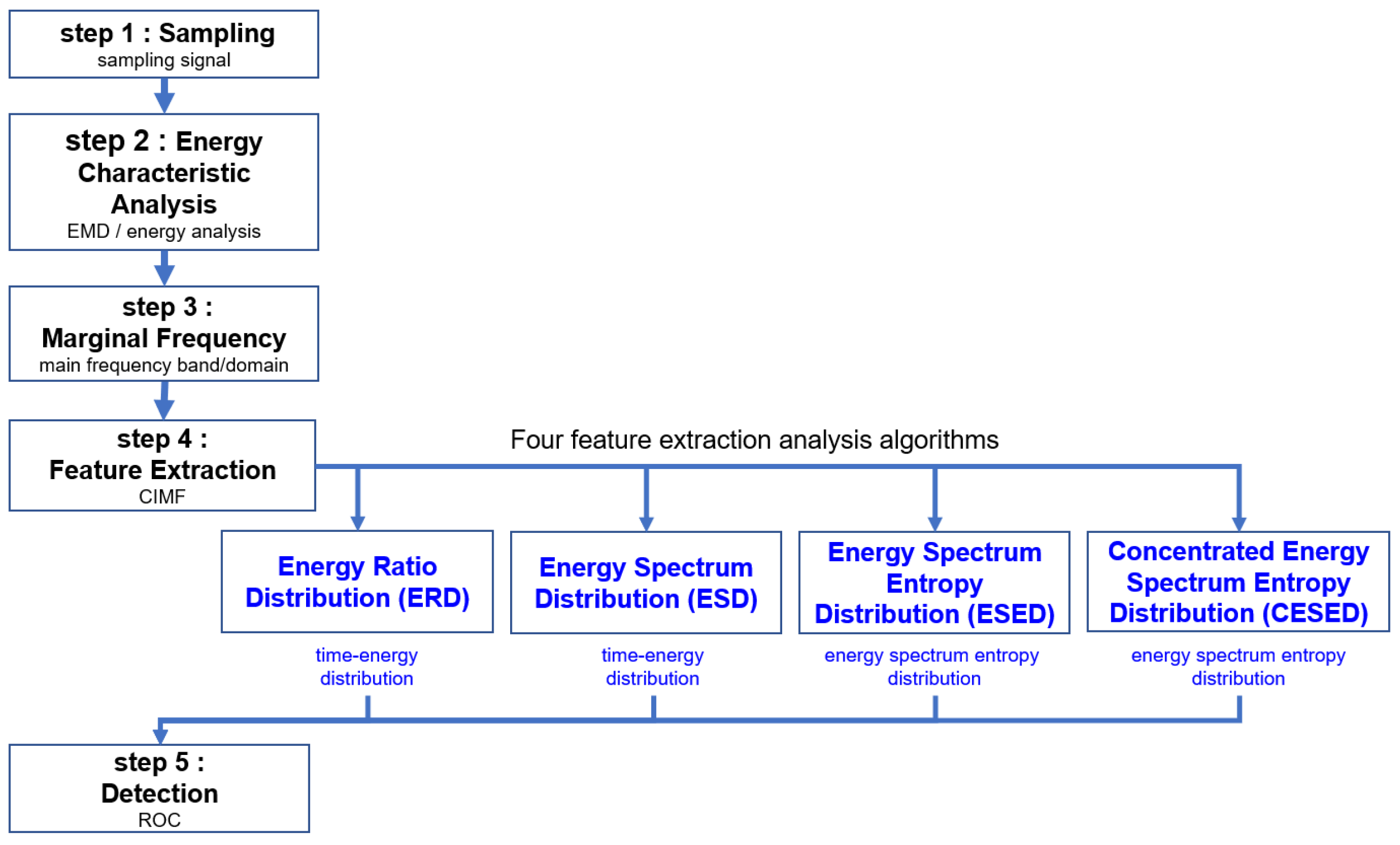
2. Method
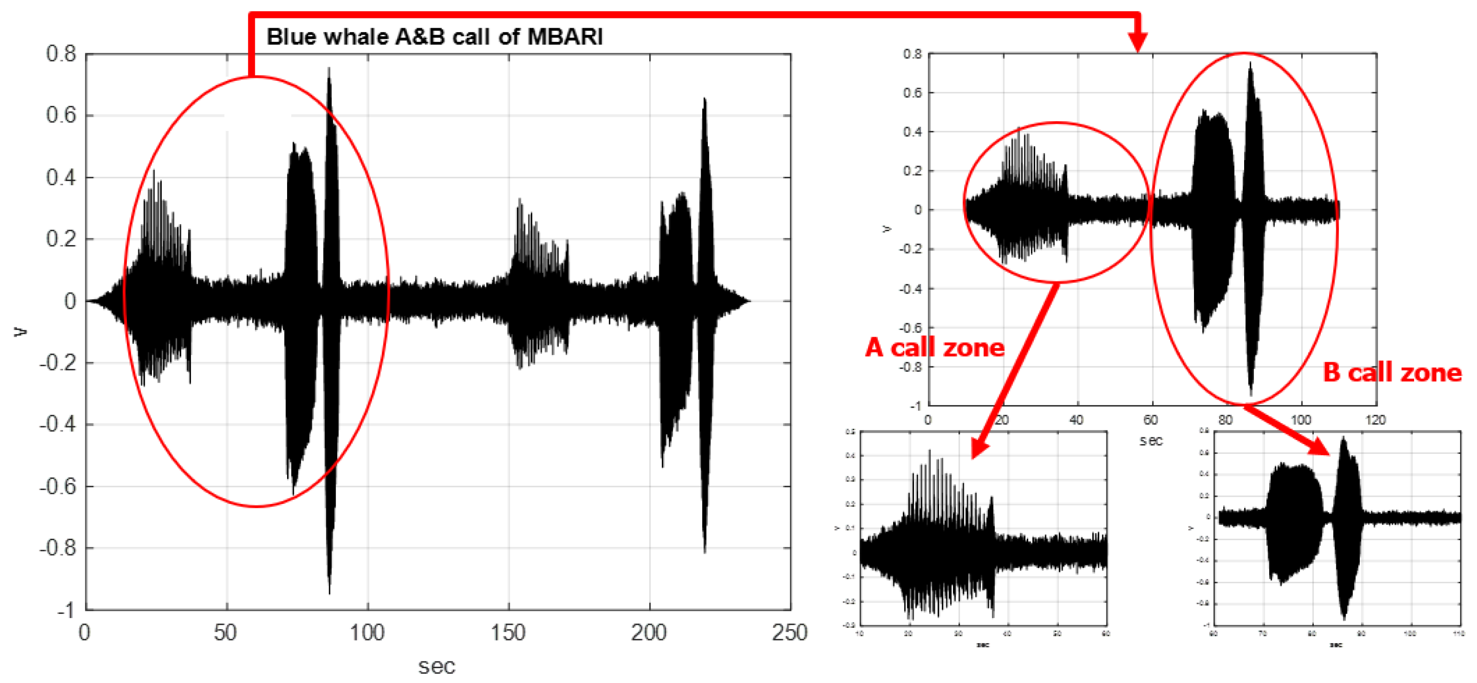
2.1. Sampling
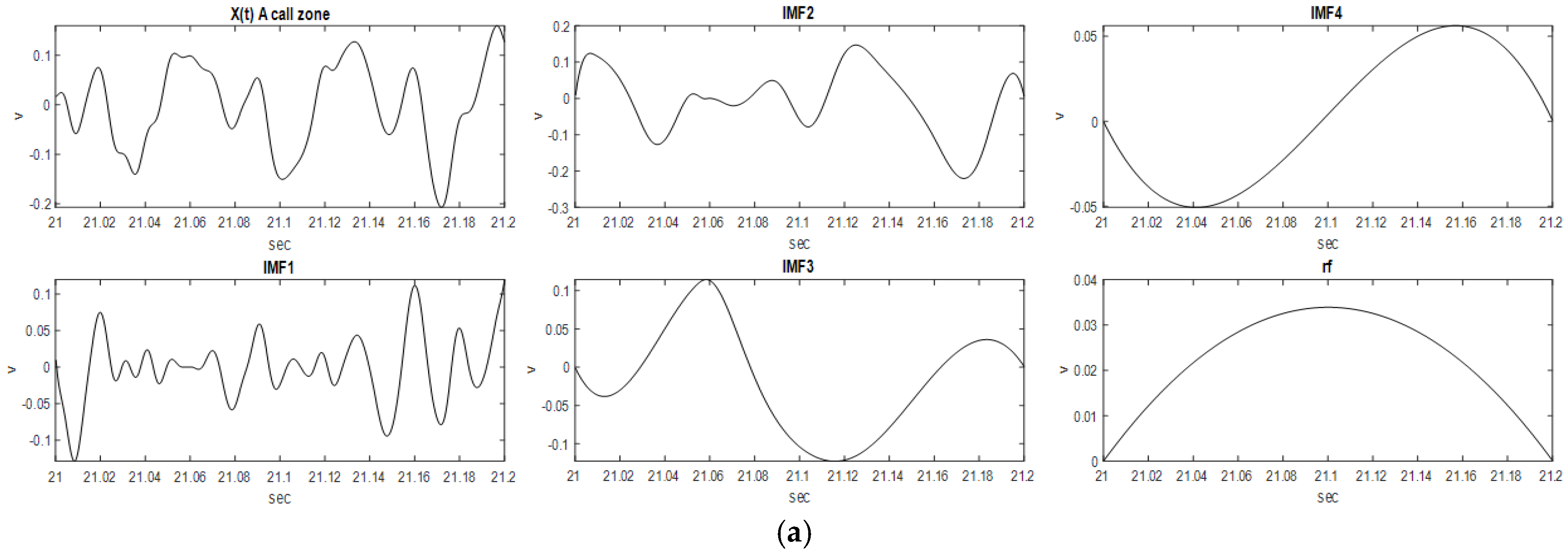
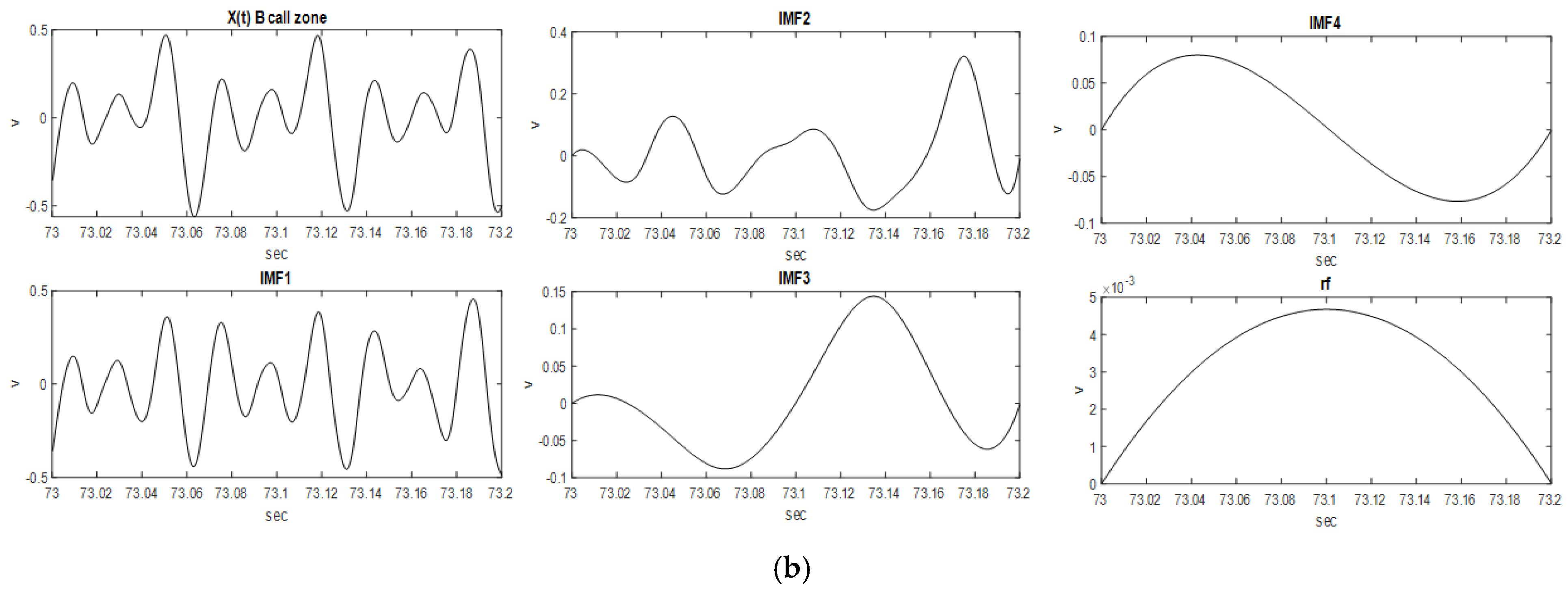
2.2. Energy Characteristics Analysis
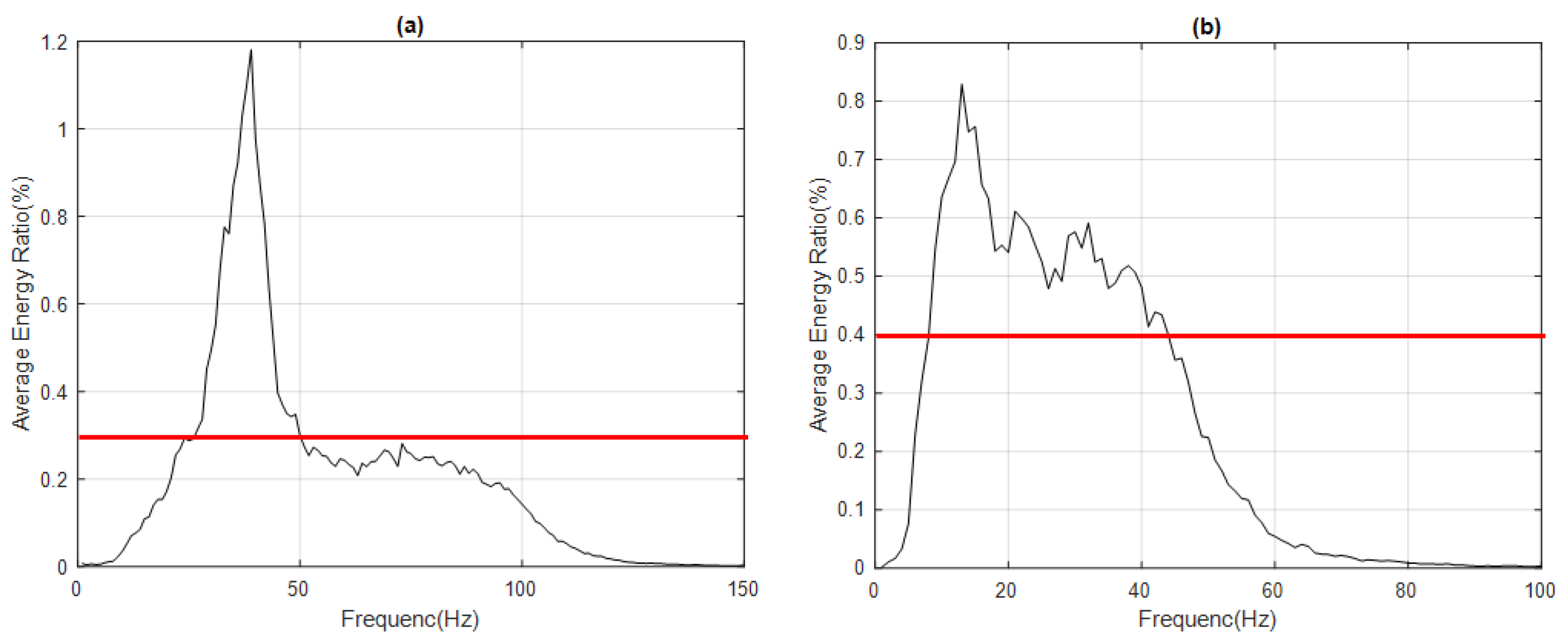
2.3. Marginal Frequency
2.4. Feature Extraction
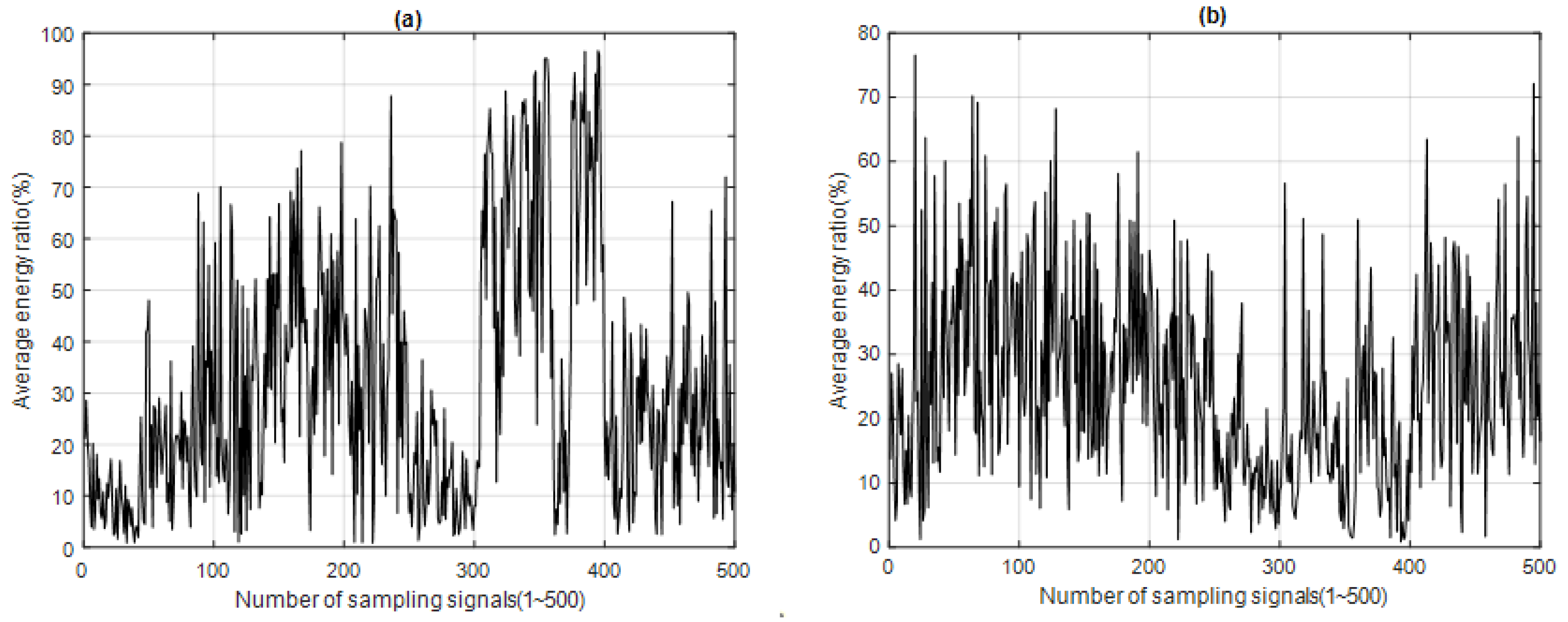
2.4.1. Energy Ratio Distribution (ERD)
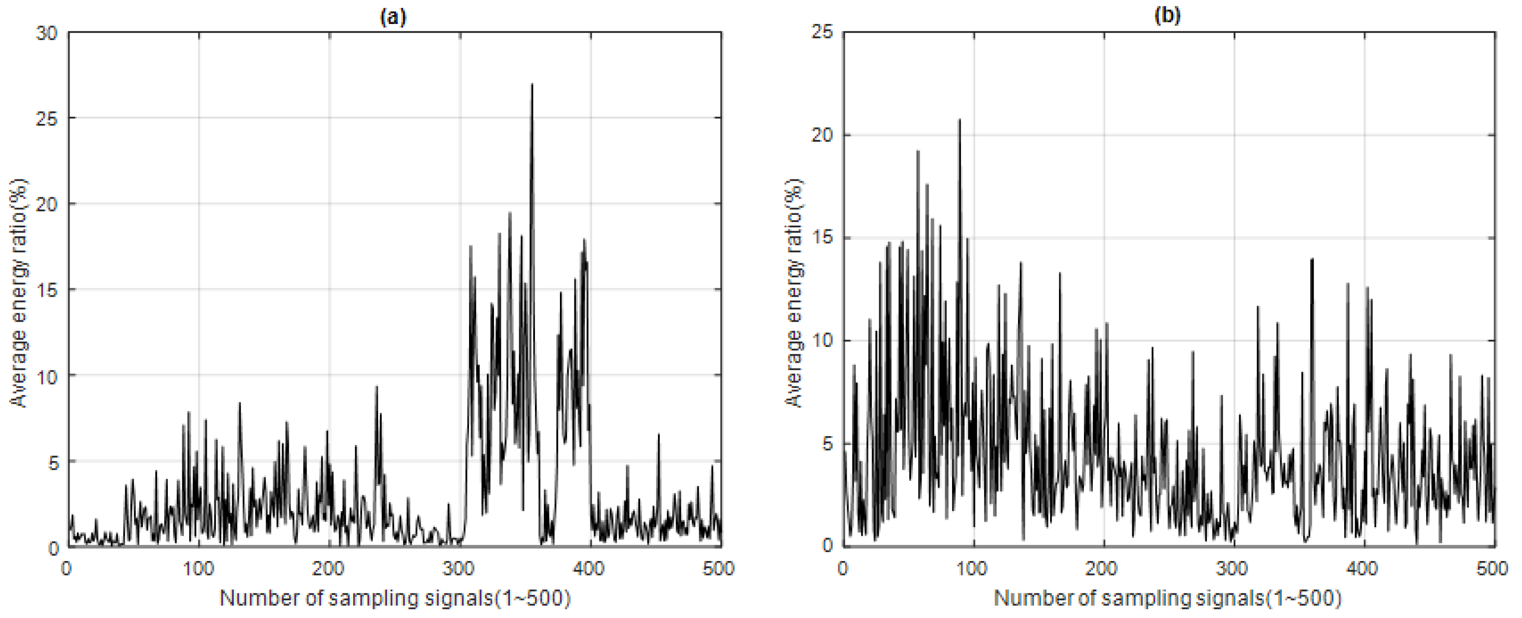
2.4.2. Energy Spectrum Distribution (ESD)
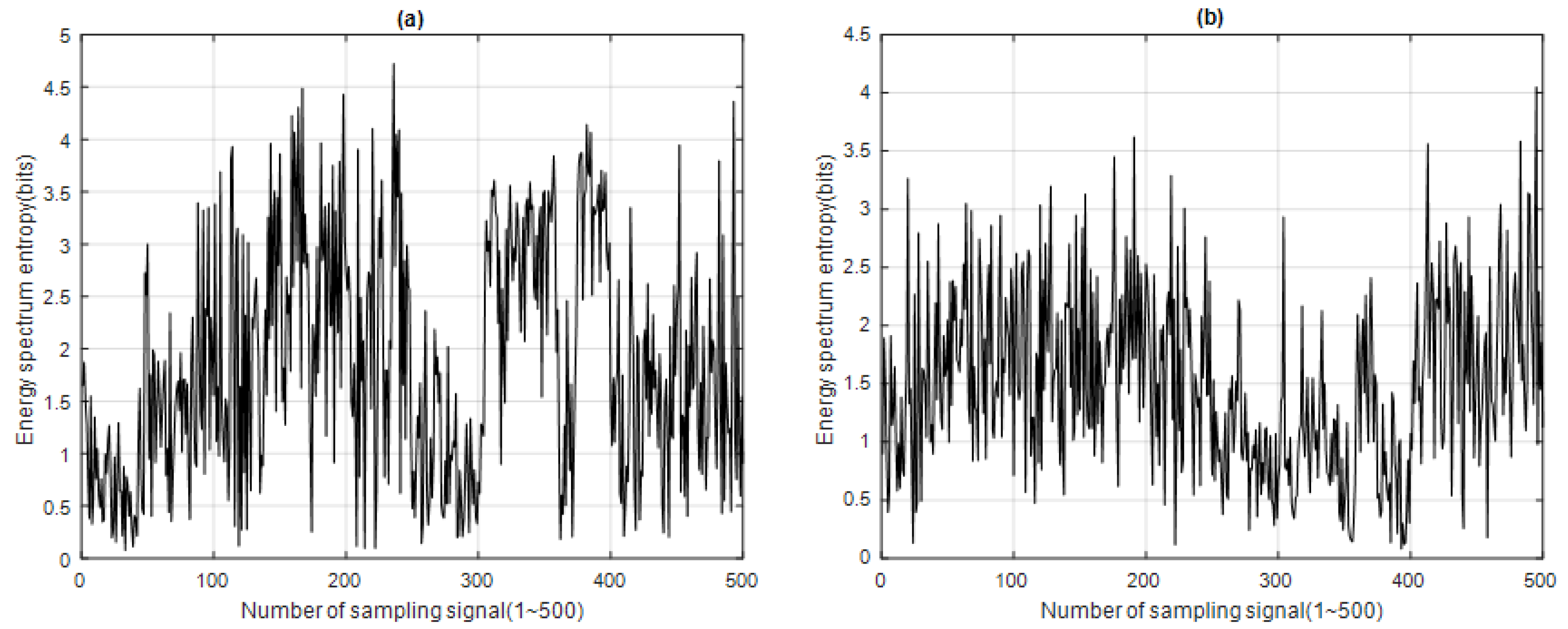
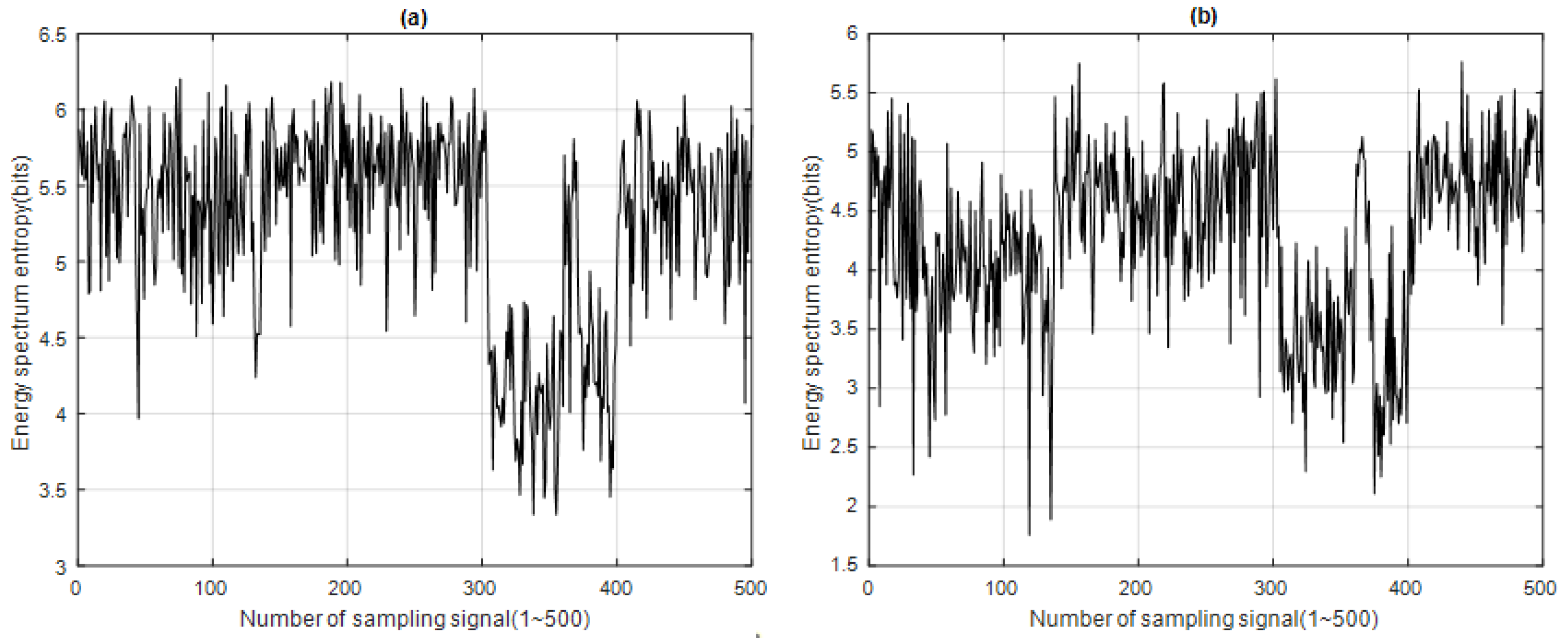
2.4.3. Energy Spectrum Entropy Distribution (ESED)
2.4.4. Concentrated Energy Spectrum Entropy Distribution (CESED)
2.5. Detection
- (1)
- Based on statistical features (medians): This approach to determining the threshold value utilizes Chebyshev’s inequality theory. According to this theory, the threshold can be set based on the energy of the sampling signal relative to the median plus a certain number of times the deviation is multiplied by a factor M [20]. This method allows for dynamic adjustment of the threshold based on the statistical features of the signal, enabling adaptation to different types of signals. Its advantages include:
- Adaptability: The threshold can be dynamically adjusted based on the statistical features of the signal, allowing it to adapt to variations in different signals;
- Robustness: By considering statistical features, threshold selection becomes more robust with respect to variations in signal characteristics, thereby improving detection performance.
- (2)
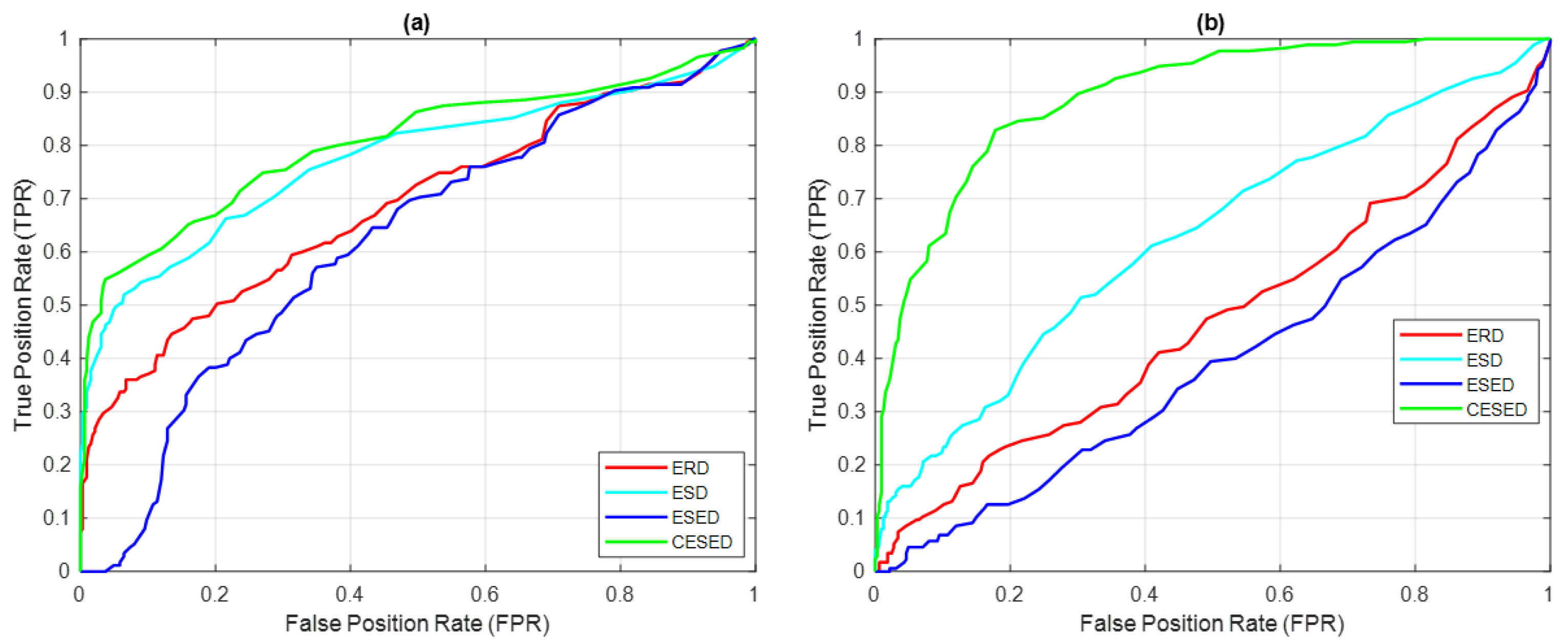
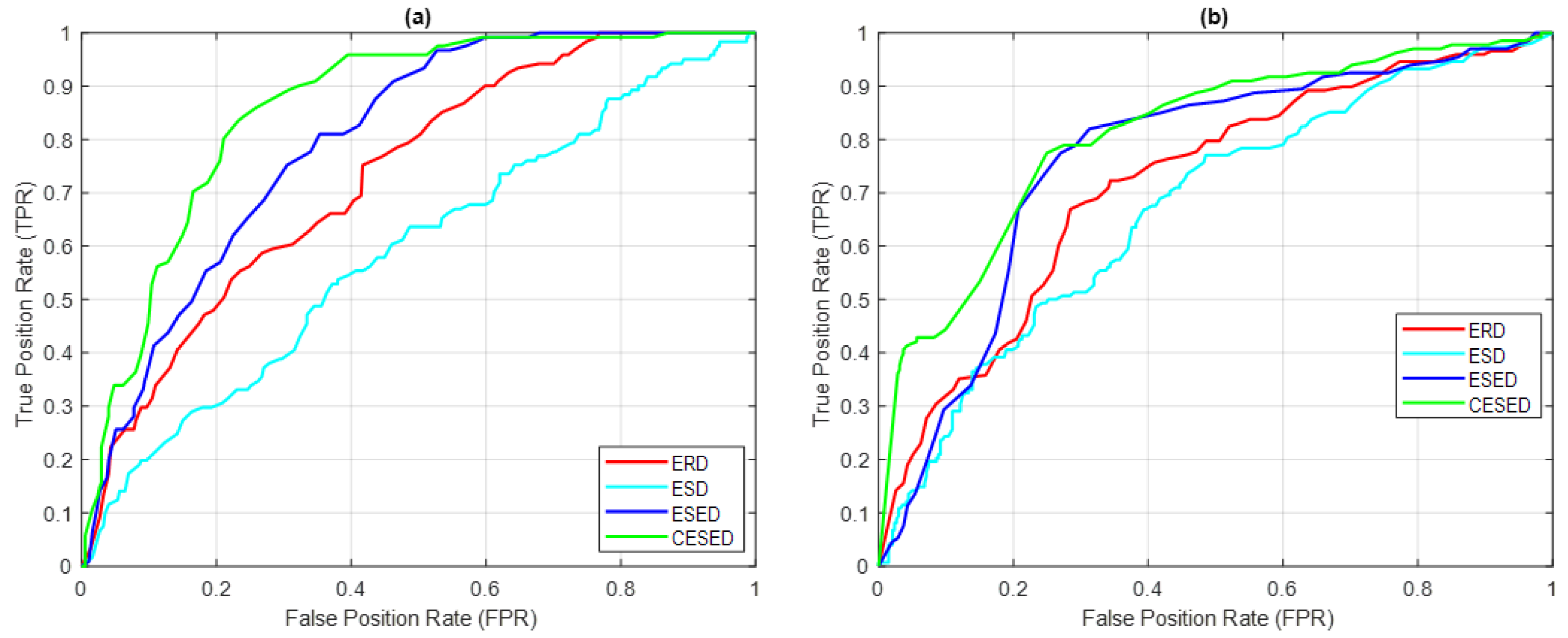
- Based on receiver operating characteristic (ROC) analysis (the optimal estimated threshold): Another criterion for selecting the threshold is by analyzing the receiver operating characteristic (ROC) curve. The ROC curve illustrates the trade-off between the true-positive rate and the false-positive rate at different threshold values. The point on the ROC curve closest to the coordinate (0,1) represents the optimal estimated result. Thus, the threshold chosen at this point can be considered the optimal estimated threshold, maximizing the system’s performance in terms of detection accuracy. By describing the process of setting the adaptive threshold based on statistical measures and selecting the optimal estimated threshold using the ROC curve, the study acknowledges the importance of threshold determination and highlights the use of adaptive techniques to enhance the detection accuracy and robustness of the system. Its advantages include:
- Performance optimization: Choosing the threshold based on the ROC curve allows identification of the optimal estimated threshold that maximizes the system’s detection accuracy. This can enhance the overall detection performance;
- Objective evaluation: The ROC curve provides a visual representation of the classifier’s performance, allowing for quantitative assessment of the balance between the true-positive rate and the false-positive rate. This objective evaluation helps in selecting a threshold that balances detection accuracy.
3. Analysis Results
4. Discussion
5. Conclusions
- (1)
- EMD can perform energy decomposition for multicomponent signals in the environment of nonstationary signals and present the energy state of signals as a function of IMFs.
- (2)
- The energy density intensity of the signal was concentrated in the main frequency domain. Energy characteristics analysis and the MF method were used to extract and analyze the signal in the main frequency domain to improve the resolution of the signal analysis.
- (3)
- Theoretical methods of EMD and entropy were used to analyze the parameters of signal data change in the signal feature extraction function distribution and the energy spectrum entropy distribution and achieve the signal detection effect.
Author Contributions
Funding
Institutional Review Board Statement
Informed Consent Statement
Data Availability Statement
Conflicts of Interest
Abbreviations
| AUC | Area under the curve |
| CESED | Concentrated energy spectrum entropy distribution |
| CIMF | Competent intrinsic mode function |
| EHO | Experienced human operator |
| EMD | Empirical mode decomposition |
| ESD | Energy spectrum distribution |
| ESED | Energy spectrum entropy distribution |
| ERD | Energy ratio distribution |
| FN | False negative |
| FP | False positive |
| HHT | Hilbert–Huang transform |
| HMM | Hidden Markov model |
| IF | Instantaneous frequency |
| IMF | Intrinsic mode function |
| MBARI | Monterey Bay Aquarium Research Institute |
| MF | Marginal frequency |
| MFCCS | Mel-scale frequency cepstral coefficients |
| NN | Neural network |
| PAM | Passive acoustic monitoring |
| rf | Residual function |
| ROC | Receiver operating characteristics |
| SE | Sample entropy |
| STFT | Short-time Fourier transform |
| SVM | Support vector machine |
| TFD | Time–frequency distribution |
| TN | True negative |
| TP | True positive |
| WT | Wavelet transform |
Appendix A

| Algorithms | Key Features | Distribution | |
|---|---|---|---|
| ERD | EIMFi(t) | The energy ratio of IMFi with the total energy | Time-energy |
| ESD | Max(EIMFi(f)) | Highest energy of spectrum with the main frequency domain (f = f1~f2) | Time-energy |
| ESED | Hsi Eij P(Eij) Hi(E) | Hilbert Spectrum of IMFi Energy distribution, i is the IMFs, j is the frequency(m~n) Probability functions Energy spectrum entropy with the total energy | Time-entropy |
| CESED | CHi(E) | Energy spectrum entropy with the main frequency domain (f = f1~f2) | Time-entropy |
| Index | Equation | Description | Parameters | Description |
|---|---|---|---|---|
| 1 | The EMD method decomposes a signal into a set of IMFs and an rf | IMFi(t) | The ith intrinsic mode function | |
| rf(t) | The residual function | |||
| 2 | The total energy is the sum of the energies of all the IMFs and rf | Etotal | The total energy of the signal | |
| 3 | The ith IMF energy ratio is divided by the total energy, Etotal | EIMFi | The ith IMF energy ratio | |
| 4 | The signal can be expressed as the sum of the real and imaginary parts | HT{IMFi(t)} | Hilbert transform for the ith intrinsic mode function | |
| Ai(t) | Amplitude of signal | |||
| θi(t) | Angular frequency of signal | |||
| 5 | By taking the derivative of the phase angle and dividing it by 2π, the instantaneous frequency of the IMF can be obtained | Fi(t) | Instantaneous frequency | |
| 6 | The sampling frequency bandwidth is f Hz, the MF (frequency–energy distribution) of the ith IMF | MFi | The ith IMF marginal frequency distribution | |
| 7 | The energy of all instantaneous frequencies is scanned and the frequency of the highest energy ratio in the main frequency domain of MF; f: f1–f2 is the main frequency domain of the MF of the sampling signal | |||
| 8 | Hilbert energy spectrum (HS; time–frequency–energy distribution) | Ei(t,f) | The energy distribution function Ei(t, f) contains the sampling time (t) and the sampling frequency (f) | |
| 9 | The energy distribution function can be expressed by the probability functions; it is normalized according to the total energy of the signal | P(Eij) | The probability functions | |
| Eij | The energy distribution, i is the IMF number, and j is the sampling frequency range m to n | |||
| 10 | The entropy of the energy spectrum of each sampling signal | H(E) | Energy spectrum entropy distribution (ESED) | |
| 11 | The energy spectrum entropy (H) of each IMFi can also be determined | |||
| 12 | The energy spectrum entropy of each IMFi in the main frequency domain, called Hicd, and the main frequency domain, which ranges from c to d | |||
| 13 | Sij, the signal energy density of the ith IMF in the sampling signal, where i is the IMF number of the sampling signal and j is the main frequency domain from a to b | |||
| 14 | The energy distribution function can be expressed by the probability functions; it is normalized according to the main frequency domain of the sampling signal | |||
| 15 | The concentrated energy spectrum entropy (CH) of each IMFi can also be determined | |||
References
- Whitlow, W.L.A.; Marc, O.L. Listening in the Ocean: New Discoveries and Insights on Marine Life from Autonomous Passive Acoustic Recorders; Springer: New York, NY, USA, 2016; pp. 1–415. [Google Scholar]
- Brekhovskikh, L.M.; Lysanov, Y.P. Fundamentals of Ocean Acoustics, 3rd ed.; Springer: New York, NY, USA, 2001; pp. 1–289. [Google Scholar]
- Usman, A.M.; Ogundie, O.O.; Versfeld, D.J.J. Review of automatic detection and classification techniques for cetacean vocalization. IEEE Access 2020, 8, 105181–105206. [Google Scholar] [CrossRef]
- Bittle, M.; Duncan, A. A review of current marine mammal detection and classification algorithms for use in automated passive acoustic monitoring. In Proceedings of the Acoustics, Victor Harbor, Australia, 17–20 November 2013. [Google Scholar]
- Zimmer, W.M.X. Passive Acoustics Monitoring of Cetaceans; Cambridge University Press: London, UK, 2011; pp. 1–368. [Google Scholar]
- Nanaware, S.; Shastri, R.; Joshi, Y.; Das, A. Passive acoustic detection and classification of marine mammal vocalizations. In Proceedings of the IEEE International Conference on Communication and Signal Processing, Melmaruvathur, India, 3–5 April 2014. [Google Scholar]
- Gillespie, D. Detection and classification of right whale calls using an ‘edge’ detector operating on a smoothed spectrogram. Can. Acoust. 2004, 32, 39–47. [Google Scholar]
- Lopatka, M.; Adam, O.; Laplanche, C.; Zarzycki, J.; Motsch, J.F. An attractive alternative for sperm whale click detection using the wavelet transform in comparison to the fourier spectrogram. Aquat. Mamm. 2005, 31, 463–467. [Google Scholar] [CrossRef]
- Adam, O. Advantages of the hilbert huang transform for marine mammals signals analysis. J. Acoust. Soc. Am. 2006, 120, 2965–2973. [Google Scholar] [CrossRef] [PubMed] [Green Version]
- Liu, J.; Li, X.K.; Ma, T.; Piao, S.C.; Ren, Q.Y. An improved hilbert-huang transform and its application in underwater acoustic signal detection. In Proceedings of the IEEE International Congress on Image and Signal Processing, Tianjin, China, 17–19 October 2019. [Google Scholar]
- Seger, K.D.; Al-Badrawi, M.H.; Miksis-Olds, J.L.; Kirsch, N.J.; Lyons, A.P. An empirical mode decomposition-based detection and classification approach for marine mammal vocal signals. J. Acoust. Soc. Am. 2018, 144, 3181–3190. [Google Scholar] [CrossRef] [PubMed] [Green Version]
- Mazhar, S.; Ura, T.; Bahl, R. Effect of temporal evolution of songs on cepstrum-based voice signature in humpback whales. In Proceedings of the IEEE International Conference on Ocean, Kobe, Japan, 8–11 April 2008. [Google Scholar]
- Pace, F.; White, P.; Adam, O. Hidden markov modeling for humpback whale (Megaptera novaeanglie) call classification. Proc. Meet. Acoust. 2012, 17, 070046. [Google Scholar]
- Murray, S.O.; Mercado, E.; Roitblat, H.L. The neural network classification of false killer whale (Pseudorca crassidens) vocalizations. J. Acoust. Soc. Am. 1998, 104, 3626–3633. [Google Scholar] [CrossRef] [PubMed] [Green Version]
- Oliver, S.K.; Fabio, F.; Yvan, S.; Nathalie, R.; Stan, M.; Samuel, G. Performance of a deep neural network at detecting north Atlantic right whale upcalls. J. Acoust. Soc. Am. 2020, 147, 2636–2646. [Google Scholar]
- Escobar-Amado, C.D.; Badiey, M.; Pecknold, S. Automatic detection and classification of bearded seal vocalizations in the northeastern Chukchi Sea using convolutional neural networks. J. Acoust. Soc. Am. 2022, 151, 299–309. [Google Scholar] [CrossRef] [PubMed]
- Ibrahim, A.K.; Zhuang, H.; Erdol, N.; Ali, A.M. A new approach for north atlantic right whale upcall detection. In Proceedings of the IEEE International Symposium on Computer, Consumer and Control, Xi’an, China, 4–6 July 2016. [Google Scholar]
- Altes, R.A. Detection, estimation, and classification with spectrograms. J. Acoust. Soc. Am. 1980, 67, 1232–1246. [Google Scholar] [CrossRef]
- Bouffaut, L.; Dreo, R.; Labat, V.; Boudraa, A.; Barruol, G. Antarctic blue whale calls detection based on an improved version of the stochastic matched filter. In Proceedings of the IEEE International Conference on European Signal Processing, Kos, Greece, 28 August–2 September 2017. [Google Scholar]
- Erbe, C.; King, A.R. Automatic detection of marine mammals using information entropy. J. Acoust. Soc. Am. 2008, 124, 2833–2840. [Google Scholar] [CrossRef] [PubMed]
- Siddagangaiaha, S.; Chen, C.F.; Hu, W.C.; Akamatsub, T.; McElligottc, M.; Lammersd, M.O.; Pierettie, N. Automatic detection of dolphin whistles and clicks based on entropy approach. Ecol. Indic. 2020, 117, 106559. [Google Scholar] [CrossRef]
- Cohen, L. Time-Frequency Analysis; Prentice Hall PTR: Englewood Cliffs, NJ, USA, 1995. [Google Scholar]
- Claasen, T.; Mechlenbrauker, W. The winger distribution—A tool for time-frequency signal analysis, parts I–III. Philips J. Res. 1980, 35, 372–389. [Google Scholar]
- Addison, P.S. The Illustrated Wavelet Transform Handbook: Introductory Theory and Applications in Science, Engineering, Medicine and Finance, 2nd ed.; CRC Press: Boca Raton, FL, USA, 2016. [Google Scholar]
- Huang, N.E.; Shen, Z.; Long, S.R.; Wu, M.C.; Shih, H.H.; Zheng, Q.; Yen, N.C.; Tung, C.C.; Liu, H.H. The empirical mode decomposition and the Hilbert spectrum for nonlinear and non-stationary time series analysis. Proc. R. Soc. Lond 1996, 454, 903–995. [Google Scholar] [CrossRef]
- Lin, C.F.; Chung, Y.C.; Zhu, J.D.; Chang, S.H.; Wen, C.C.; Parinov, I.A.; Shevtsov, S.N. The energy based characteristics of sperm whale clicks using the hilbert huang transform analysis method. J. Acoust. Soc. Am. 2017, 142, 504–511. [Google Scholar] [CrossRef] [PubMed]
- Wen, C.S.; Lin, C.F.; Chang, S.H. Extraction of energy characteristic of blue whale vocalization base on empirical mode decomposition. Sensors 2022, 22, 2737. [Google Scholar] [CrossRef] [PubMed]
- Shannon, C.E. A mathematical theory of communication. Bell Syst. Tech. J. 1948, 27, 379–423. [Google Scholar] [CrossRef] [Green Version]
- Monterey Bay Aquarium Research Institute. Available online: https://www.mbari.org/soundscape-blue-whale-behavior/ (accessed on 11 April 2023).
- Urazghildiiev, I.R.; Clark, C.W. Detection performances of experienced human operators compared to a likelihood ratio based detector. J. Acoust. Soc. Am. 2007, 122, 200–204. [Google Scholar] [CrossRef] [PubMed]
- Van Trees, H.; Kristine, L.B. Detection, Estimation, and Modulation Theory PART I—Detection, Estimation, and Filtering Theory, 2nd ed.; WILEY Publisher: Hoboken, NJ, USA, 2013; pp. 17–110. [Google Scholar]
- Ponomarenko, A.; Salin, M. Marine mammal calls detection in acoustic signals via gradient boosting model. Proc. Meet. Acoust. 2021, 44, 010001. [Google Scholar]
- Scripps Institution of Oceanography UCSD, Scripps Whale Acoustic Lab. Available online: http://voicesinthesea.ucsd.edu/ (accessed on 11 April 2023).
- Kuroshio Ocean Education Foundation. Available online: https://www.kuroshio.org.tw/ (accessed on 11 April 2023).


| IMFi | IMF1 | IMF2 | IMF3 | IMF4 | IMF5 | IMF6 | IMF7 |
|---|---|---|---|---|---|---|---|
| Average energy ratio (%) | 31.92 | 25.09 | 19.29 | 12.14 | 6.62 | 1.90 | 0.21 |
| IMFi | Threshold | Frequency of Highest Energy Ratio (Hz) | Main Frequnecy Band (Hz) | Main Frequency Domain (Hz) |
|---|---|---|---|---|
| IMF1 | 0.3 | 39 | 27~49 | 1~150 |
| IMF2 | 0.3 | 13 | 9~43 | 1~100 |
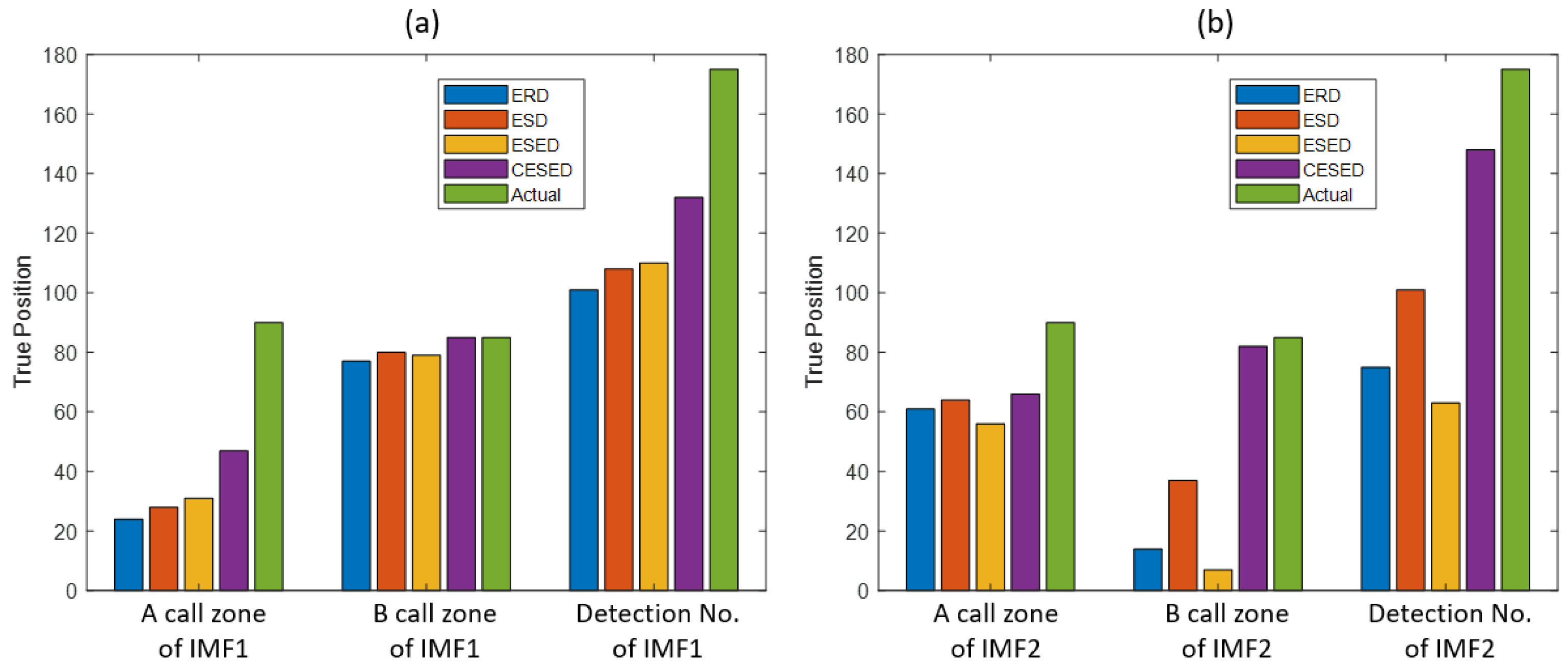
| IMF1 Threshold (Median) | True Position (TP) | False Position (FP) | ||||||
|---|---|---|---|---|---|---|---|---|
| A Call Zone Number | B Call Zone Number | Detection Number | Detection Ratio (TPR) | A Call Zone Number | B Call Zone Number | False Alarm Number | False Alarm Ratio (FPR) | |
| ERD | 35 | 80 | 115 | 65.71% | 86 | 50 | 136 | 41.72% |
| ESD | 47 | 83 | 130 | 74.29% | 70 | 38 | 108 | 33.23% |
| ESED | 37 | 79 | 116 | 66.29% | 86 | 47 | 133 | 40.80% |
| CESED | 47 | 85 | 132 | 75.43% | 40 | 60 | 100 | 30.37% |
| IMF2 Threshold (Median) | True Position (TP) | False Position (FP) | ||||||
|---|---|---|---|---|---|---|---|---|
| A Call Zone Number | B Call Zone Number | Detection Number | Detection Ratio (TPR) | A Call Zone Number | B Call Zone Number | False Alarm Number | False Alarm Ratio (FPR) | |
| ERD | 69 | 17 | 86 | 49.14% | 96 | 73 | 169 | 52.15% |
| ESD | 107 | 40 | 107 | 61.14% | 77 | 56 | 133 | 40.92% |
| ESED | 62 | 12 | 74 | 42.29% | 97 | 86 | 183 | 56.44% |
| CESED | 72 | 85 | 157 | 89.71% | 64 | 34 | 98 | 30.66% |
| IMF1 (the Optimal Estimated Threshold) | True Position (TP) | False Position (FP) | ||||||
|---|---|---|---|---|---|---|---|---|
| A Call Zone Number | B Call Zone Number | Detection Number | Detection Ratio (TPR) | A Call Zone Number | B Call Zone Number | False Alarm Number | False Alarm Ratio (FPR) | |
| ERD | 24 | 77 | 101 | 57.71% | 73 | 27 | 100 | 30.67% |
| ESD | 28 | 80 | 108 | 61.71% | 45 | 17 | 62 | 19.08% |
| ESED | 31 | 79 | 110 | 62.86% | 78 | 35 | 113 | 34.66% |
| CESED | 47 | 85 | 132 | 75.43% | 40 | 60 | 100 | 30.37% |
| IMF2 (the Optimal Estimated Threshold) | True Position (TP) | False Position (FP) | ||||||
|---|---|---|---|---|---|---|---|---|
| A Call Zone Number | B Call Zone Number | Detection Number | Detection Ratio (TPR) | A Call Zone Number | B Call Zone Number | False Alarm Number | False Alarm Ratio (FPR) | |
| ERD | 61 | 14 | 75 | 42.86% | 84 | 66 | 150 | 46.32% |
| ESD | 64 | 37 | 101 | 57.71% | 71 | 53 | 124 | 38.15% |
| ESED | 56 | 7 | 63 | 36.00% | 81 | 69 | 151 | 46.32% |
| CESED | 66 | 82 | 148 | 84.57% | 46 | 23 | 69 | 21.17% |
| Species | Sampling Frequency (Hz) | Sampling Time (ms) | Number of Sampled | CIMF | Average Energy Ratio | Main Frequency Domain (Hz) | Optimal Estimated Threshold | Performance Metric | ERD | ESD | ESED | CESED |
|---|---|---|---|---|---|---|---|---|---|---|---|---|
| Blue whale [27] | 4800 | 200 | 500 | 2 | 25.09% | 1~100 | 4.38 | AUC Accuracy Precision Recall F1 score | 0.4621 49.90% 31.19% 42.83% 37.41% | 0.6162 60.40% 44.89% 57.71% 50.50% | 0.3894 47.50% 29.44% 36.00% 32.39% | 0.8979 80.84% 68.20% 84.57% 84.57% |
| Bowhead whale [29] | 4800 | 200 | 500 | 2 | 34.73% | 1~100 | 2.55 | AUC Accuracy Precision Recall F1 score | 0.7388 60.61% 35.77% 76.86% 48.82% | 0.5944 58.99% 30.84% 54.55% 39.40% | 0.8061 68.89% 42.53% 77.69% 54.97% | 0.8980 81.45% 67.83% 58.79% 80.17% |
| Bryde’s whale [29] | 2400 | 200 | 500 | 5 | 29.59% | 1~100 | 1.10 | AUC Accuracy Precision Recall F1 score | 0.7254 69.60% 49.02% 67.57% 56.82% | 0.6678 62.55% 42.61% 66.22% 51.85% | 0.7735 72.99% 50.48% 78.95% 61.58% | 0.8320 74.28% 51.98% 78.95% 62.69% |
| Dolphin whistle [31] | 96,000 | 200 | 200 | 1 | 68.03% | 2000~8000 | 8.36 | AUC Accuracy Precision Recall F1 score | 0.8800 87.00% 44.12% 68.18% 53.57% | 0.8945 86.00% 42.86% 81.82% 56.25% | 0.6777 61.31% 18.39% 72.73% 29.36% | 0.7582 79.00% 29.17% 63.64% 40.00% |
| Pattern dolphin click [32] | 44,100 | 200 | 300 | 1 | 30.96% | 1~1000 | 7.10 | AUC Accuracy Precision Recall F1 score | 0.7812 67.67% 51.85% 81.55% 63.40% | 0.6525 58.47% 43.40% 66.35% 52.47% | 0.7953 75.00% 62.73% 66.99% 64.79% | 0.7589 69.44% 54.35% 72.12% 61.98% |
Disclaimer/Publisher’s Note: The statements, opinions and data contained in all publications are solely those of the individual author(s) and contributor(s) and not of MDPI and/or the editor(s). MDPI and/or the editor(s) disclaim responsibility for any injury to people or property resulting from any ideas, methods, instructions or products referred to in the content. |
© 2023 by the authors. Licensee MDPI, Basel, Switzerland. This article is an open access article distributed under the terms and conditions of the Creative Commons Attribution (CC BY) license (https://creativecommons.org/licenses/by/4.0/).
Share and Cite
Wen, C.-S.; Lin, C.-F.; Chang, S.-H. EMD-Based Energy Spectrum Entropy Distribution Signal Detection Methods for Marine Mammal Vocalizations. Sensors 2023, 23, 5416. https://doi.org/10.3390/s23125416
Wen C-S, Lin C-F, Chang S-H. EMD-Based Energy Spectrum Entropy Distribution Signal Detection Methods for Marine Mammal Vocalizations. Sensors. 2023; 23(12):5416. https://doi.org/10.3390/s23125416
Chicago/Turabian StyleWen, Chai-Sheng, Chin-Feng Lin, and Shun-Hsyung Chang. 2023. "EMD-Based Energy Spectrum Entropy Distribution Signal Detection Methods for Marine Mammal Vocalizations" Sensors 23, no. 12: 5416. https://doi.org/10.3390/s23125416