1. Introduction
The Internet of Things (IoT) is transforming our lives and workplaces, presenting unparalleled opportunities to improve efficiency, reduce costs, enhance safety, and drive innovation across a broad range of industries and applications. From smart homes and cities to healthcare, transportation, and industrial automation, IoT is reshaping how we engage with the world. One promising application of IoT technology is the use of unmanned aerial vehicles (UAVs) for effective data collection, enabling real-time monitoring and analysis in various contexts [
1,
2]. In particular, the healthcare industry is poised to experience significant economic growth worldwide by 2025, with estimates projecting annual growth between USD 1.1 trillion and 2.5 trillion due to the adoption and integration of IoT technology [
3].
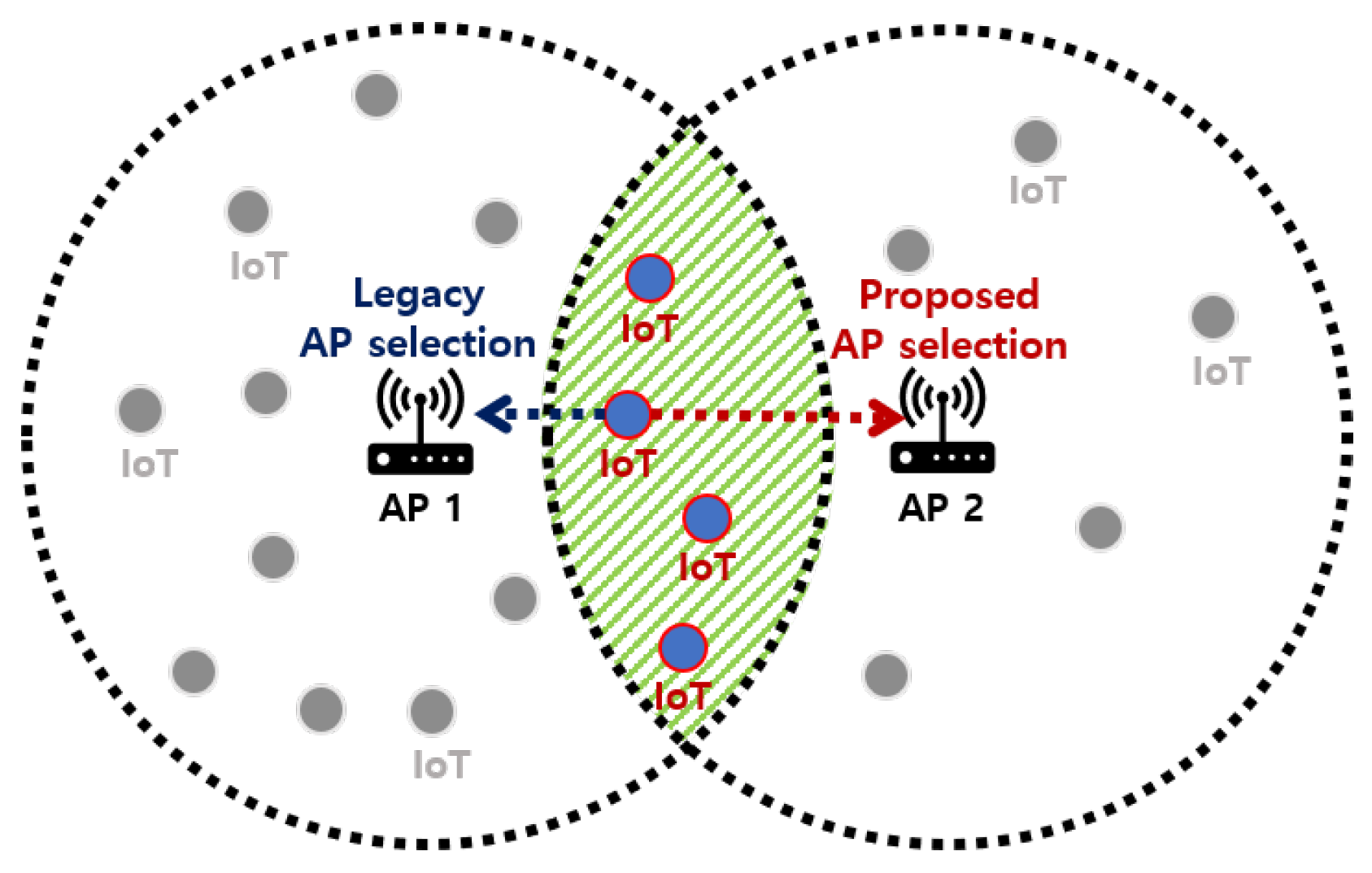
As the traffic on a Wi-Fi network increases, the cells covered by the network’s access point (AP) become smaller and more crowded. As a result, mobile terminals (MTs), including IoT devices, are present within multiple overlapping cells in Wi-Fi networks [
4]. In this scenario, MTs typically connect to the AP with the strongest signal, which can result in contention and packet collisions during transmission due to the concentration of the devices on particular APs. Consequently, these repetitive transmissions can disrupt energy efficiency and increase latency at the device. Additionally, non-crowded APs are underutilized, which leads to lower overall network performance. Therefore, it is important to address the issue of selecting the optimal AP that considers IoT devices’ energy efficiency and latency in a multi-coverage Wi-Fi network environment.
There are two types of AP selection schemes in Wi-Fi networks: distributed and centralized. In a traditional distributed scheme, an MT selects an AP based on the received signal strength indication (RSSI) values between the MT and several available APs [
5]. However, biased AP connections can occur when many MTs want to connect to a particular AP, which leads to load imbalance and poor quality of service (QoS) for MTs, including low throughput and latency performance [
6]. Some studies have attempted to solve this problem by using the combination of RSSI values and other parameters [
7,
8], but distributed AP selection methods have limitations in addressing load balancing due to the limited information that MTs can obtain [
9,
10,
11].
To address these issues, centralized AP selection methods have been proposed [
12,
13,
14]. The centralized approach for AP selection involves the AP choosing the most suitable AP based on factors such as RSSI value and achievable throughput. This method can help to reduce the problem of unbalanced load and enhance network performance. However, this approach does not take into account the uplink traffic and the energy efficiency of IoT devices. When aiming to provide IoT services, it is crucial to consider the uplink traffic and the energy efficiency of IoT devices because the performance (e.g., reliability, durability, etc.) highly depends on the transmission activity of the IoT devices. For example, in healthcare IoT services, uplink traffic, including sensed IoT data, is frequently transmitted to the server, and the amount of uplink traffic is much more significant than that of downlink traffic. Therefore, rather than considering downlink traffic, the consideration of uplink traffic is more important. In addition, the frequent replacements of IoT devices due to the limited battery capacity is the most significant challenge for implementing good quality IoT service.
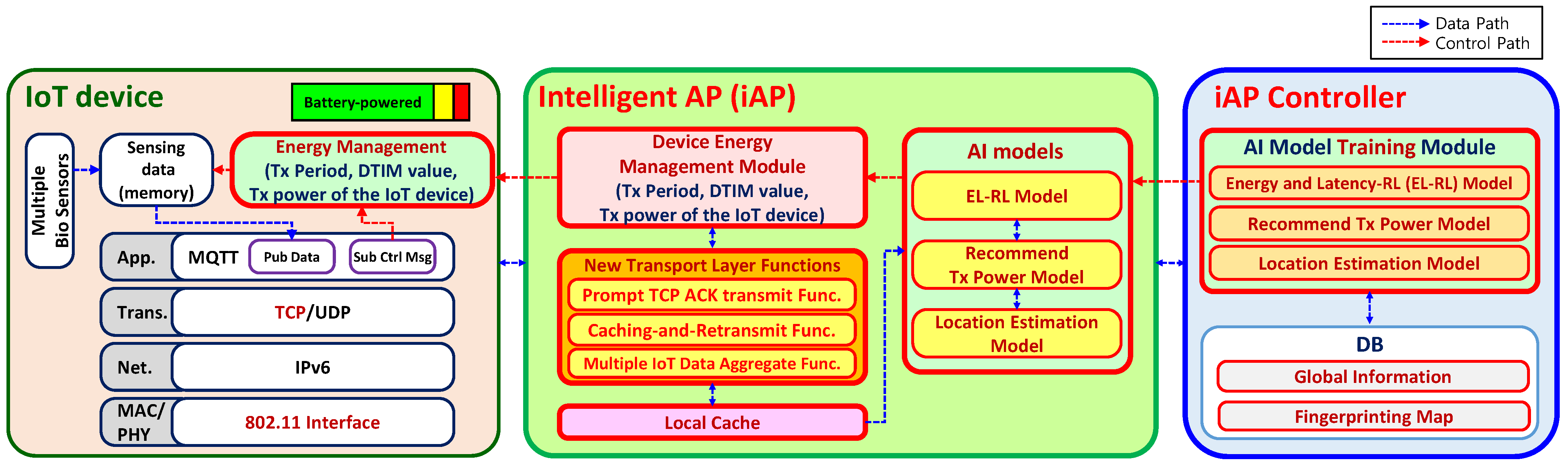
To solve the problems mentioned above, in [
15] (our previous study on the iAP system), we proposed the iAP system that increases the energy efficiency of IoT devices when transmitting uplink IoT data after the AP connection procedure. However, we have recognized that the procedures for the initial AP selection and connection establishment also cause a large energy consumption of IoT devices, especially in crowded network environments. Such real-time connection dynamics between MTs and APs occur without the knowledge of future connections. The selection of an AP has a significant impact on network performance, specifically in terms energy efficiency, as it is influenced by factors such as the uplink traffic of APs and the distance between APs and their connected MTs. However, relying solely on the received signal strength indicator (RSSI) between the MT and AP is inadequate for achieving optimal connections. Moreover, the number of possible cases for connections between MTs and APs grows exponentially with the number of MTs, resulting in a large search space. To effectively explore this space while considering the influence of the current AP selection on future network performance, the adoption of a reinforcement learning algorithm is essential.
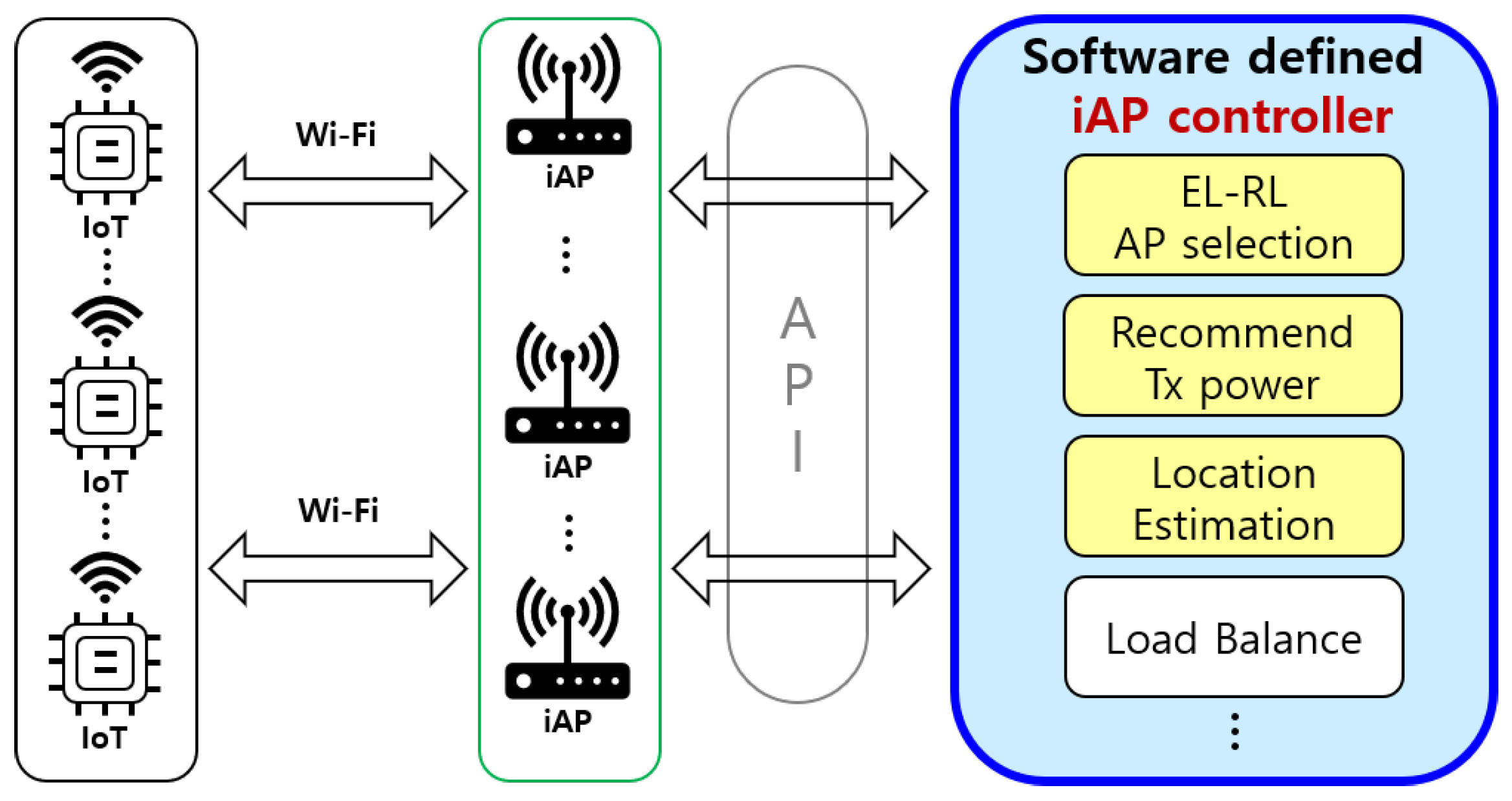
Therefore, in this paper, we propose an energy-efficient AP connection method using an intelligent AP (iAP) system [
15] to increase the lifespan of IoT devices; particularly, we focus on an AP selection and connection method before transmitting uplink IoT data to achieve much better energy efficiency for IoT devices.
The main contributions of this paper are as follows:
This paper proposes a novel energy-efficient AP selection scheme to increase the lifespan of IoT devices. To achieve this, we design an AP control system architecture that selects the optimal AP and controls operating parameters.
We propose a new Energy and Latency Reinforcement Learning (EL-RL) model for optimal AP selection. The EL-RL model utilizes RSSI values and the number of connected IoT devices as input sequences for the AI model, with the aim of addressing the load-unbalancing problem and enhancing the energy efficiency of IoT devices. To the best of our knowledge, this represents the first attempt to consider the real-time connection dynamics and energy efficiency of IoT devices in the context of optimal AP selection.
Based on the newly defined collision probability considering the retransmission of IoT devices, we design the energy consumption and latency estimation model of the overall IoT devices in Wi-Fi networks.
We also analyzed the energy consumption and latency of IoT devices using a proposed energy-efficient AP selection scheme with an EL-RL model. Through extensive simulations, the proposed scheme achieved significant improvements, including a maximum of in energy efficiency, in uplink latency, and a -times improvement in the expected lifespan of IoT devices, compared to legacy AP selection schemes.
2. Related Works
Enhancing the energy efficiency of IoT devices is of paramount importance as it enables the provision of a diverse range of IoT services while simultaneously minimizing energy consumption. Significant research efforts have been devoted to this area, as evidenced by notable studies [
16,
17,
18,
19,
20]. These works have made significant contributions to the understanding and development of energy-efficient solutions for IoT devices, offering valuable insights and strategies for improving their performance in terms of energy consumption and sustainability.
When multiple access points are overlapped, the selection of an appropriate AP becomes a critical concern. An energy-efficient AP selection method is required to address this challenge and enhance the energy efficiency and QoS for IoT devices in IoT services. As a result, numerous studies have focused on investigating AP selection schemes in both decentralized and centralized approaches [
5,
6,
7,
8,
9,
10,
11,
12,
13,
14]. These research endeavors aim to provide effective solutions for optimizing AP selection and improving the overall throughput and QoS of IoT devices in diverse IoT services (
Table 1).
In legacy distributed AP selection schemes, the MT selects the AP with the strongest signal [
5,
9], which causes an unbalanced load across the network. In [
9], the authors used an RSSI interval overlap degree determination method to improve positioning accuracy, but it did not address the load-unbalancing problem. Other AP selection schemes that utilize RSSI value and achievable throughput parameters also have limitations in AP load balancing and network utilization [
7,
11]. While in [
7] the authors used a multi-armed bandits algorithm to enhance downlink throughput, it did not consider uplink traffic. In [
11], the authors increased downlink throughput using RSSI value and achievable throughput, but the authors did not consider uplink traffic and energy consumption of MTs. Even centralized AP selection approaches primarily focus on downlink throughput [
12,
13], without considering uplink performance and collision probability. In [
12], the authors used RSSI value and achievable throughput to select the optimal AP using a centralized approach, but the authors did not consider uplink traffic and energy efficiency. In [
13], the authors used estimated RSSI values, which are obtained by a long short-term memory (LSTM) algorithm to improve positioning accuracy while reducing computational load and enhancing noise robustness, but the authors did not consider uplink traffic and energy efficiency. In general, AP selection studies have mainly emphasized increasing downlink performance rather than considering the uplink traffic and energy efficiency of IoT devices.
For more robust and durable IoT services, new AP selection proposals are necessary because IoT devices, which are the main component of the service, are sensitive to energy and uplink delay [
15]. Therefore, a new energy-efficient AP selection scheme is required to overcome the problem of biased connection to a particular AP, which increases the collision probability of the network. Particularly, the biased connection can result in an increased amount of retransmissions at IoT devices, leading to higher energy consumption and uplink latency. Therefore, in this paper, we propose a new method that considers such problems to improve the performance of Wi-Fi networks.
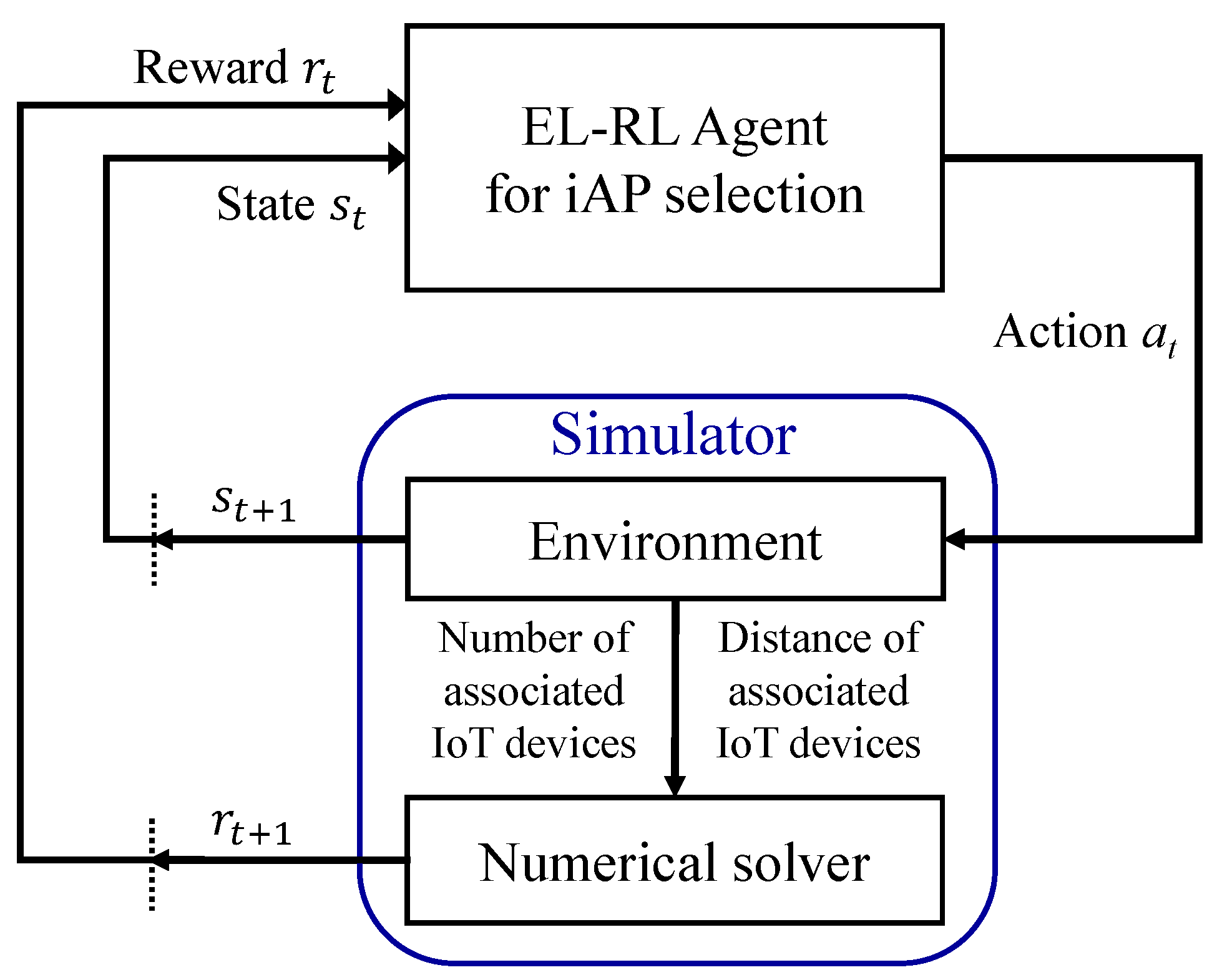
4. Energy and Latency Reinforcement Learning (EL-RL) Model
The proposed Energy and Latency Reinforcement Learning (EL-RL) model is illustrated in
Figure 6. The model is designed for iAP selection, where the environment sends state information in the form of
to the EL-RL agent. The state
is determined based on the RSSI between the IoT device and the candidate iAP, as well as the number of MTs currently connected to the iAP. At this stage, action
represents the candidate iAP to connect the IoT device. The numerical solver then computes the reward
, taking into account the number of connected IoT devices and their distances from the chosen iAP. Additionally, the reward is calculated based on the average energy consumption and latency of IoT devices. Thus, the EL-RL model aims to minimize the average energy consumption and latency of all connected IoT devices, which is set as the objective function. The EL-RL agent receives the reward
and selects a new action, and this process continues iteratively until the agent obtains the maximum reward through reinforcement learning. The notations used in the EL-RL model are defined as follows:
State,
- –
Global network information (, ) where ).
- –
Candidate iAP set of the IoT device i where .
Action,
- –
Select of the IoT device i where .
- –
where subscript is the number of candidate iAPs for connecting the IoT device i among all iAPs.
Reward (penalty),
- –
+ .
- –
where is the weight for avg. energy consumption and is the weight for avg. latency.
Policy
- –
Minimize the objective function .
In addition, the proposed iAP control system includes a location estimation ML model. This model employs a fingerprint method, which estimates location based on RSSI values by comparing them with reference point values stored in the database. The fingerprint method is widely recognized as the most suitable method for indoor positioning [
21,
22]. Once the location is estimated, the distances to each candidate iAP are calculated, and the recommended Tx power values are determined according to the adaptive Tx power equation (Equation (
A1)) in the
Appendix A [
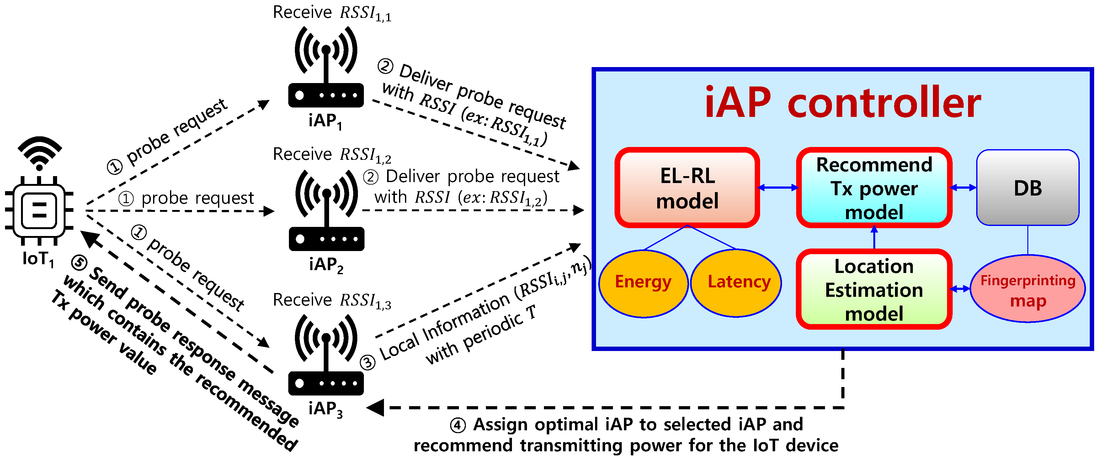
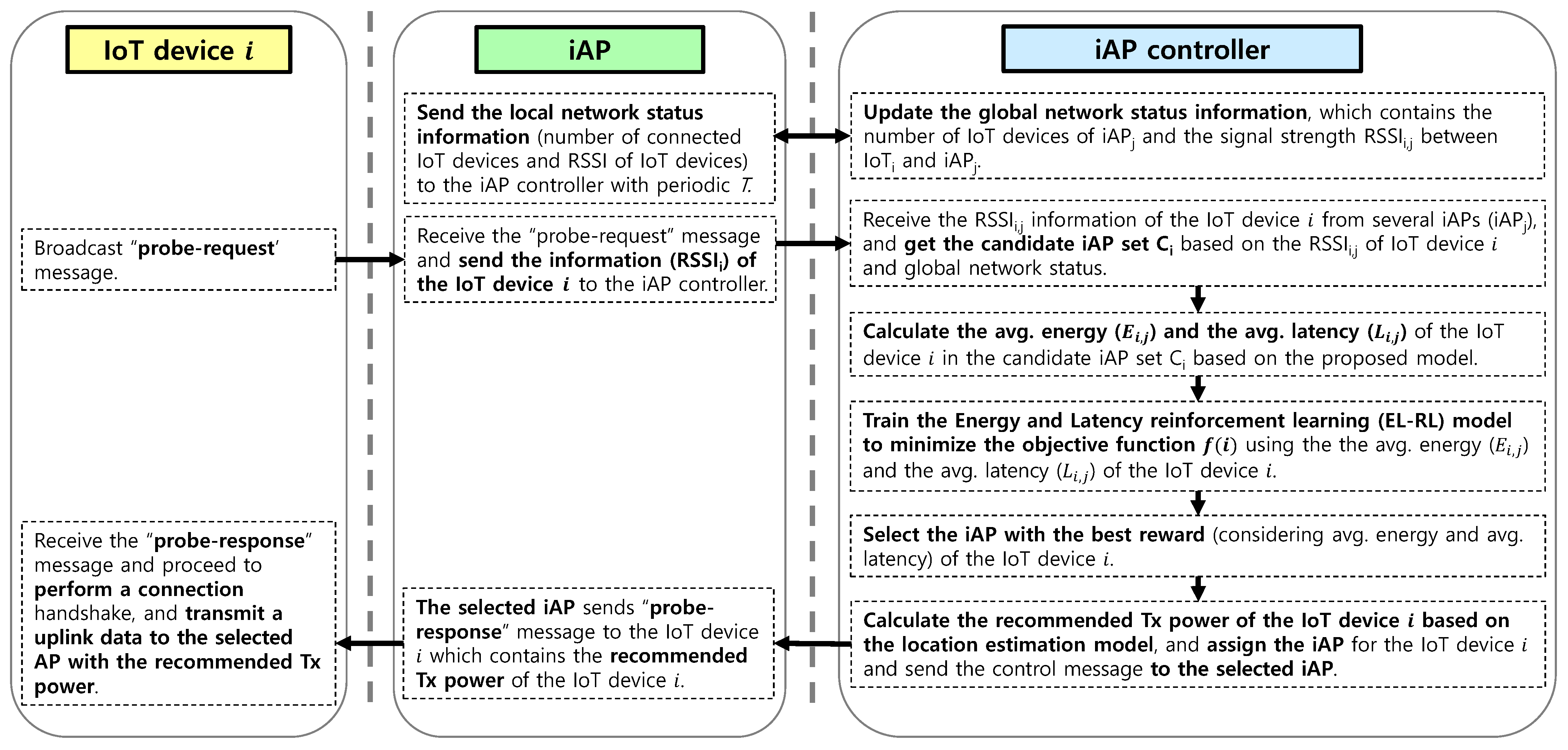
15]. The iAP controller selects the optimal AP based on the EL-RL model and sends the recommended transmitting power to the IoT device. The iAP controller then updates the localization ML model and EL-RL model.
In the training procedure of the EL-RL model, each training data instance is obtained whenever a new connection is established between a MT and an AP. Each training data instance consists of the state
, which includes information such as the RSSI between the MT and AP and the number of already connected MTs for each AP. Additionally, it contains the action
representing the selected AP for the connection and the reward
associated with the chosen action in terms of network performance, such as latency and energy efficiency. To facilitate the training process, the training data is constantly stored in the iAP controller’s storage as new connections are made. From this dataset, a batch of training data is randomly selected for training the EL-RL model. This random selection helps ensure a diverse and representative sample of the training instances. To further enhance the learning process, the reward for each action in the selected training data is adjusted using the Proximal Policy Optimization (PPO) algorithm [
23]. By adjusting the rewards, the model can better estimate the impact of each action on future network performance. During each epoch of training, the model’s parameters are iteratively updated using randomly chosen training data. This iterative process allows the model to gradually improve its performance and adapt to various network conditions. The training continues for several epochs until the total reward converges, indicating that the model has learned an optimal policy for AP selection.
4.1. Collision Probability
The energy consumption caused by traffic retransmissions resulting from packet collisions is demonstrated in
Figure 7. When an IoT device and any other IoT devices try to simultaneously transmit a packet during the first transmission attempt from the IoT device perspective, a collision occurs between the transmitted packets, and a timeout for the IoT device occurs because an ACK(Acknowledgement) packet has not been received. Once the channel becomes idle again, the IoT device attempts a second transmission using a random backoff time within the double contention window size. The same process applies to the collisions encountered during the second through sixth transmission attempts. If a collision happens even on the seventh transmission attempt, the packet is discarded, and there is no further retransmission attempt.
To examine the energy consumption attributed to retransmissions, we conduct mathematical calculations of collision probabilities based on realistic collision simulations. As per the IEEE 802.11 standardization, we consider that the IoT device could transmit the same packet a total of seven times, which includes the initial transmission attempt. Hence, the maximum number of retransmission attempts (
m) is six [
24,
25], the minimum contention window size
is 31 time slots, the maximum contention window size
is 1023 time slots, and the maximum number of recursive attempts to increase
is 6 [
24,
25]. We define the collision probability for each transmission attempt as
and the transmission attempt probability as
in follows.
Therefore, the transmission probability of the
nth transmission attempt,
is given by Equation (
1),
In this paper, a collision occurs when more than one IoT devices share the same time slot for attempting uplink transmissions. For example, when one device among
N devices is trying to transmit within a certain time slot, another device among
devices may try to transmit simultaneously. We take into account the concurrent transmission attempt in the following collision model. The transmission collision probability is formulated from a new perspective in Equation (
2),
- –
where
- –
where
- –
where
This collision probability is calculated by considering the packet collision probability within a single arbitrary time slot. Additionally, this collision probability considers the actual collision probability for ML, which can be solved numerically. Concerning the transmitting devices at an arbitrary time slot, the number of devices attempting the first transmission in that time slot is represented by , and the number of devices attempting the second transmission is expressed as . Likewise, describes the number of devices attempting nth transmission in that time slot for . In addition, is the number of devices with no transmission attempt in the same time slot.
The collision probability is defined as the sum of the values multiplied by the number of cases in which collision can happen and the transmission attempt probability. Here, if there is no transmission from any device at that time slot, the has a value of 0, and it is considered that no collision has occurred. Furthermore, is defined as the sum of all attempted transmission probabilities. The collision probability based on these actual collisions was calculated with numerical techniques.
4.2. Energy and Latency of IoT Devices
In this subsection, we present the average energy consumption and the average latency model of IoT devices based on the collision probability. The average energy consumption of IoT devices can be obtained as the sum of the product of the probability of all transmission attempts, the probability of successful transmission without collision, and the energy consumption value according to the
nth transmission attempt. The average energy consumption of IoT devices is given as Equation (
3),
The energy consumed by the
nth transmission attempt is the sum of the product of the operation time of each operation mode and the power used in that operation mode as follows in Equation (
4).
The total Tx mode time according to the transmission attempt consists of data transmission time and ACK transmission time in Equation (
5). The data transmission time can be obtained by multiplying the number of transmission attempts by the time required to send one transmission data, and the ACK transmission time can be obtained by the time required to send an L2ACK message once.
where
is a 104 bytes,
is a 54 bytes,
B is a 160 kHz, and
is a 40 dB [
15].
The total Rx (Receive) mode time according to the transmission attempt is given by
where
is a 337
s,
is a 44
s [
12], and
is a
s [
15]. The time calculated in Rx mode is the sum of the ACKtime time value, the beacon reception time value, and the product of the number of times sent so far and the time set by ACKtimeout.
The total sleep mode time according to the transmission attempt is given by
where
is a 1 s of the transmission period. The total sleep mode time per transmission attempt can be obtained by subtracting the Tx mode time and the Rx mode time from the period.
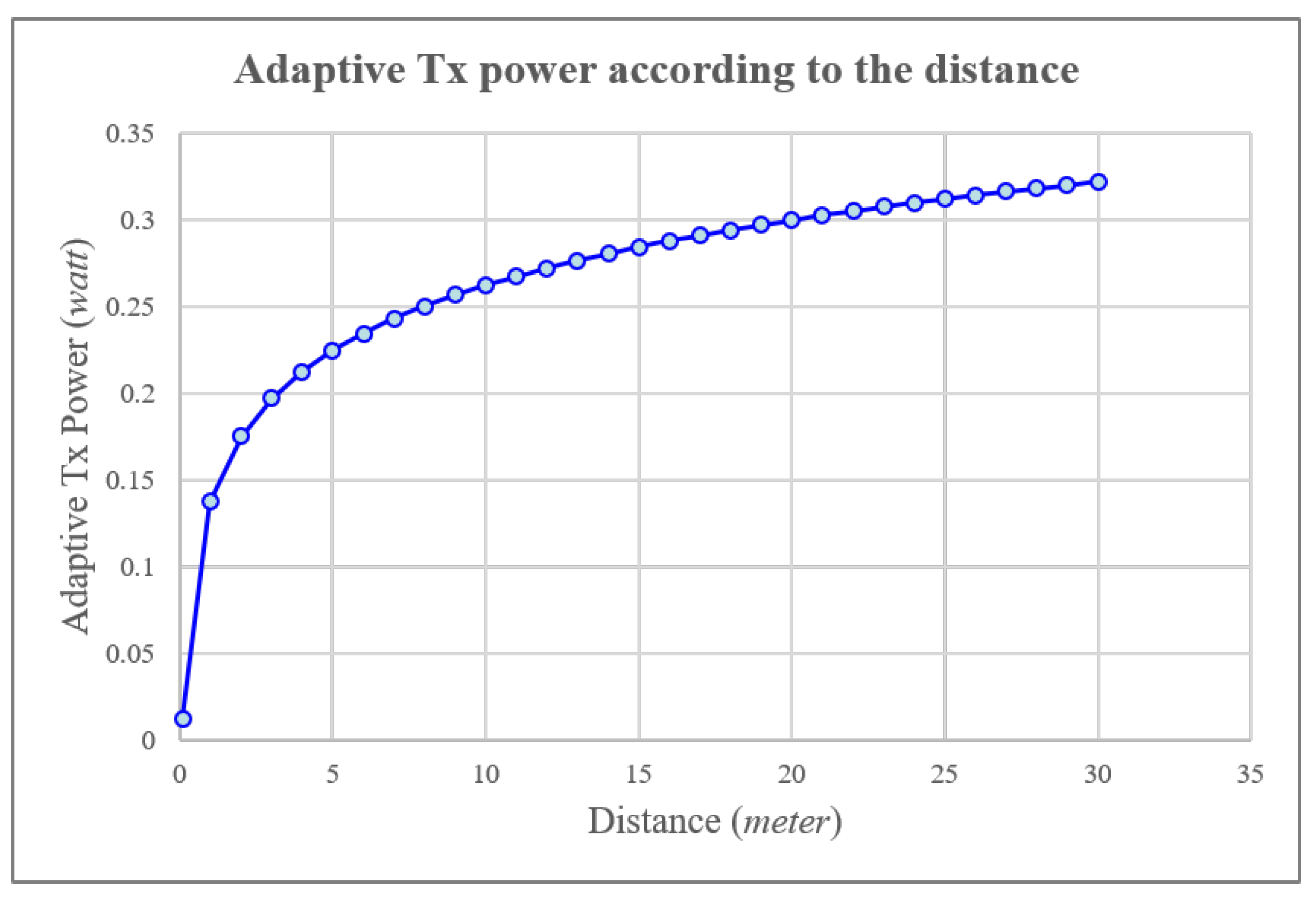
In addition, the adaptive Tx power according to the distance,
, can be obtained as Equation (
A1) in the
Appendix A [
15]. The average uplink latency of IoT devices is calculated by the below Equation (
8). The average latency is composed of the average backoff time, the average transmission time for successful delivery, and the average collision time for transmission failure according to the
nth transmission attempts,
The average backoff time of
nth transmission attempts is given by
where
is a 20
s, and
is a 16 as a default value [
12]. The average transmission time for the successful delivery of
nth transmission attempts is given by
where SIFS is a 10
s,
is a 44
s, and DIFS is a 50
s [
12]. The average collision time for transmission failure of
nth transmission attempts is given by
where
is a 337
s, and DIFS is a 50
s [
12].
To calculate the average consumed energy of an IoT device, we use the RSSI values and the number of IoT devices that are connected to the iAPs. Moreover, to calculate the average latency of an IoT device, we use the number of IoT devices that are connected with iAPs for load balancing. The objective function of the proposed EL-RL model has defined below in Equation (
12),
where
and
are the weight of average energy consumption and average latency, respectively. The goal of the objective function is to minimize the weighted sum of the average energy value and average latency value.
5. Performance Evaluation
The simulator uses Python and the PyTorch library for the PPO algorithm implementation [
26]. The parameter settings for simulation are shown in
Table 3.
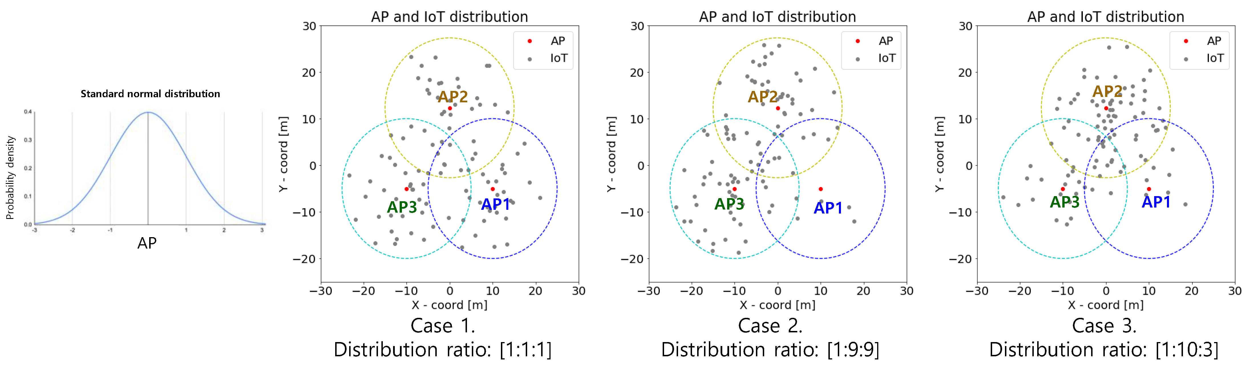
For the simulation, we assume the total number of APs is three, the distance between the APs is 20 m, and the cell coverage is 15 m. In addition, it is assumed that the IoT devices in each APs are normally distributed with respect to the iAP location, which is placed at the center of the cell. The distribution ratio of IoT between APs are assumed to be [1:1:1], [1:9:9], and [1:10:3]. These represent hotspot scenarios: balanced scenario, two hotspots scenario, and one hotspot scenario, respectively. The total numbers of IoT devices applied to the simulation are 50, 100, 150, and 200. Reinforcement learning of the EL-RL model is performed based on the PPO algorithm, which shows the best performance and fastest learning in various fields [
27] (
Figure 8).
The reason for using the PPO algorithm is as follows. First, it is rare for a sequence to produce a similar state because the state in a sequence is defined by the distance between the IoT device and the AP and the number of devices connected to the AP. Second, in order to train EL-RL model from numerous amount of various sequences, we must carefully consider the effect of current actions on future actions, i.e., the final return value. Therefore, we implement an advantage actor-critic-based PPO algorithm as a value-based algorithm that can efficiently consider the return value for the current action.
The agent of the proposed EL-RL model is based on the PPO algorithm. The state, action, reward weight values, and epoch of the EL-RL model for the simulation are as follows.
State:
- –
represent the RSSI value of the at the .
- –
represent the number of connected IoT devices in the .
Action:
- –
represent selection to .
- –
represent selection to .
- –
represent selection to .
Reward weight value:
- –
: Average energy consumption of .
- –
: Average uplink latency of .
Epoch: 200
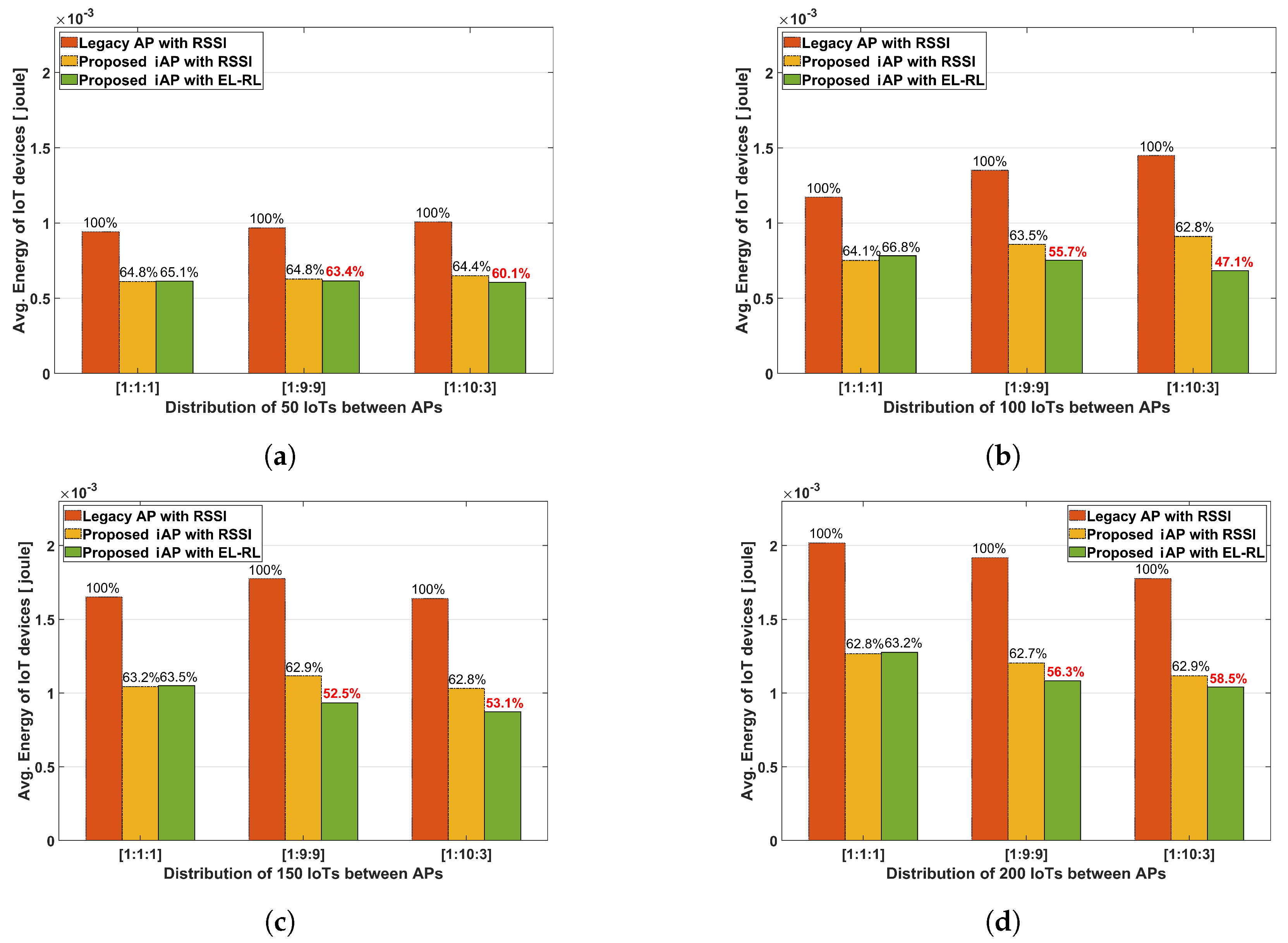
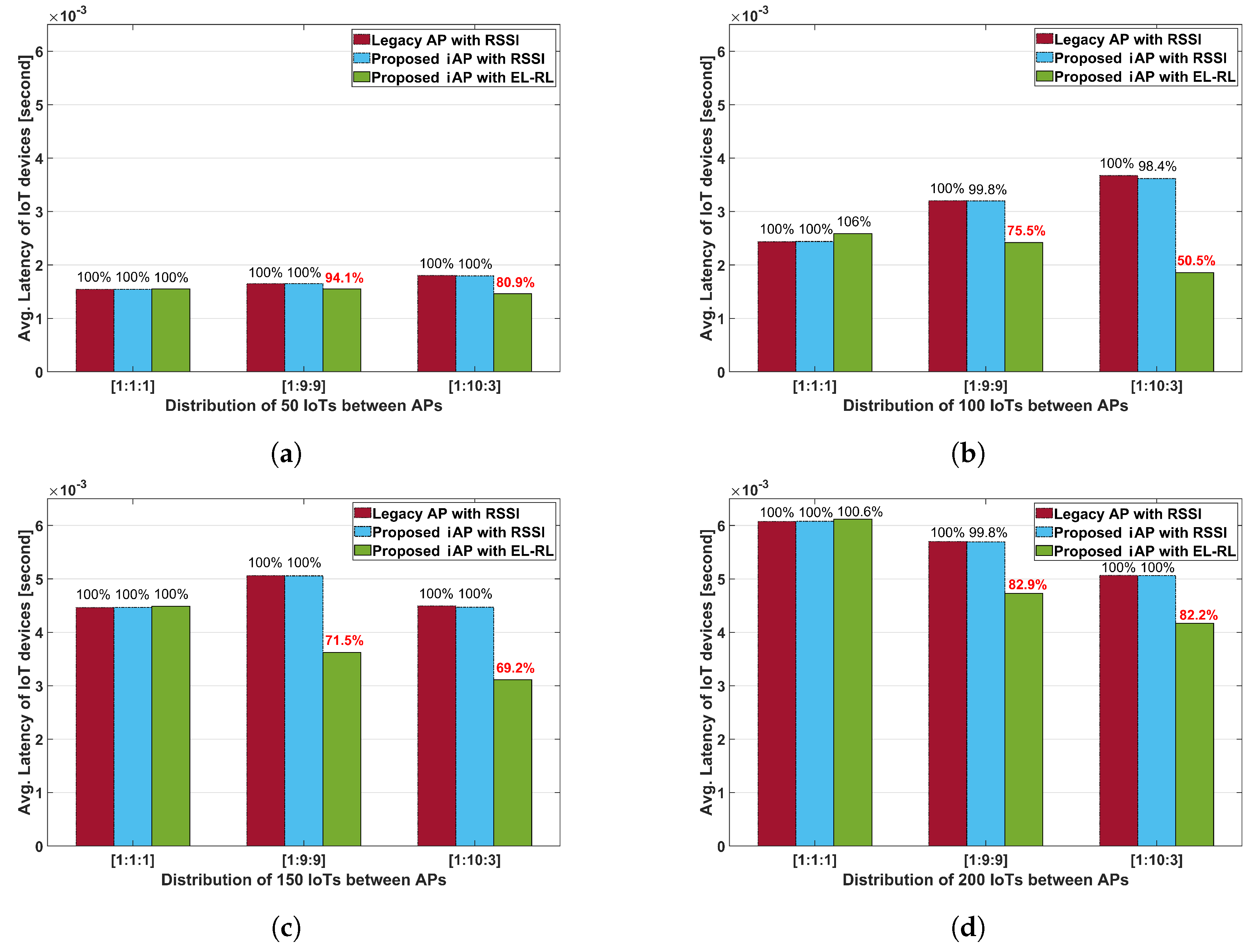
We compare three AP selection models for performance evaluation. First, the legacy AP selection model that only uses RSSI value to select AP is presented as ‘legacy AP with RSSI’. Second, the proposed iAP selection model that only uses RSSI value to select iAP with an adaptive Tx power is expressed as ‘proposed iAP with RSSI’. Last, the proposed iAP selection model that uses the EL-RL agent to select iAP is denoted as ‘proposed iAP with EL-RL’. With three AP selection models, we consider three cases regarding distribution ratios of IoT devices between APs as follows.
Case 1: refers to the balanced case (the distribution ratio between APs is [1:1:1]).
Case 2: refers to the two hotspots case (the distribution ratio between APs is [1:9:9]).
Case 3: refers to the one hotspot case (the distribution ratio between APs is [1:10:3]).
The results for each model in all experiments are the average value obtained from 500 simulations.
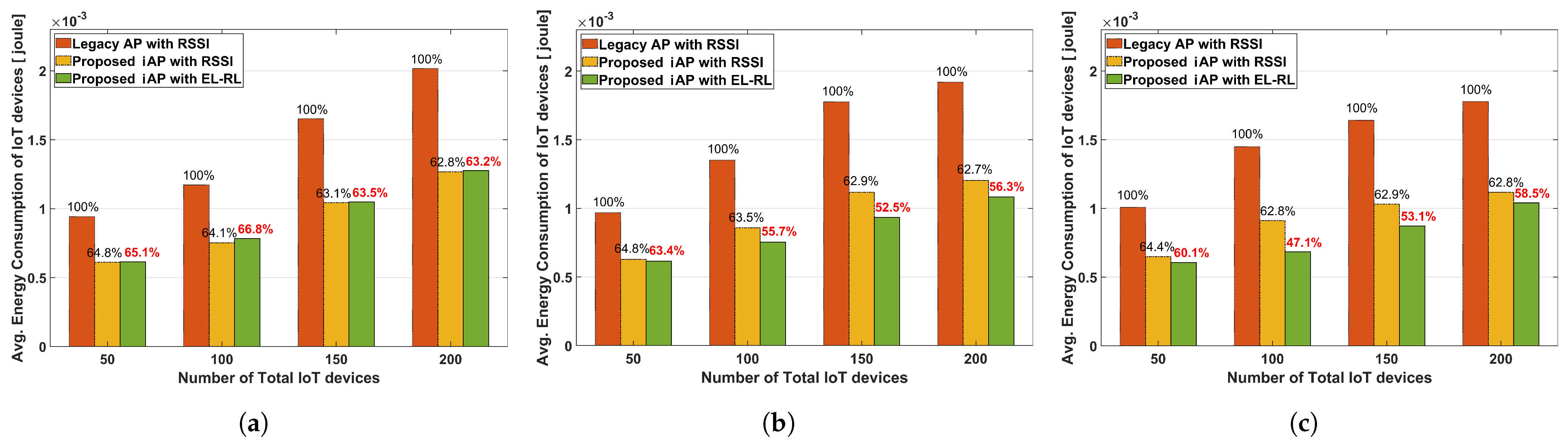
Figure 9 presents the average energy consumption of IoT devices according to the distribution ratio between APs. In all cases, the average energy consumption of IoT devices shows an increasing trend as the number of devices increases. For Case 1, the energy consumption performance of the two proposed iAP models (namely ‘proposed iAP with RSSI’ and ‘proposed iAP with EL-RL’) are better than that of the ‘legacy AP with RSSI’ model, but the energy consumption values of the two models are comparable as shown in
Figure 9a. Since Case 1 is already load-balanced, it shows similar performance between the two proposed models. However, the two proposed iAP models demonstrate lower energy consumption, at 63∼66%, compared to the legacy AP model because of the adaptive Tx power and the prompt ACK reception function in the iAP system. In Case 2 and Case 3, as shown in
Figure 9b,c, respectively, the average energy consumption of IoT devices increases with the increasing number of IoT devices, a similar trend to Case 1. In Case 2, where there are two hotspot APs, the two proposed iAP models exhibit energy consumption performance ranging from 62% to 65% compared to the legacy AP model. On the other hand, in Case 3, where there is only one hotspot AP, the two proposed iAP models demonstrate better performance in terms of energy consumption ranging from 47% to 64% compared to the legacy AP model. Especially the ‘proposed iAP with EL-RL’ model performs the best in Case 3, exhibiting energy consumption of only
compared to the ‘legacy AP with RSSI’ model, with a total of 100 IoT devices. This is because the ‘proposed iAP with EL-RL’ model has a better load-balancing effect that reduces retransmission energy.
Figure 10 displays the average energy consumption of IoT devices for cases with respect to the different numbers of IoT devices. The results indicate that the two proposed iAP models outperform the legacy AP model in terms of energy consumption performance. Particularly, the ‘proposed iAP with EL-RL’ model demonstrates the best energy consumption performance, achieving an energy reduction of
in the 1:10:3 distribution of 100 IoT devices. This outcome is due to the ‘proposed iAP with EL-RL’ model’s load-balancing scheme, which selects the optimal AP while taking into account both energy consumption and latency.
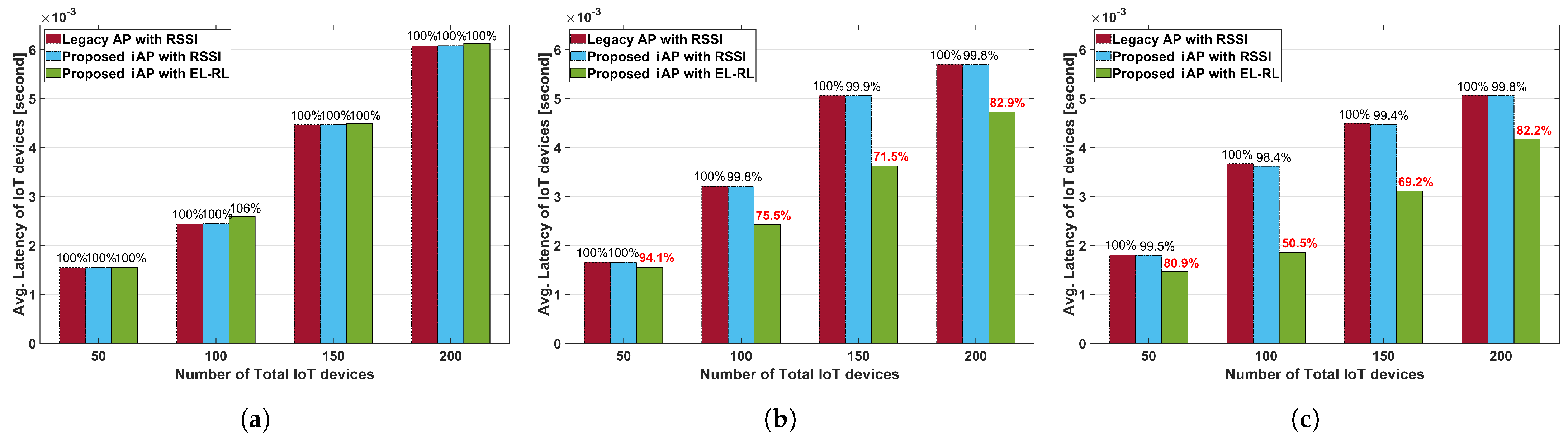
Figure 11 presents the average uplink latency of IoT devices according to the distribution ratio between APs.
Figure 11a shows the average uplink latency of IoT devices for Case 1. The average uplink latency of each model increases as the number of IoT devices increases due to retransmissions resulting from packet collisions. However, the two proposed iAP models exhibit almost the same average uplink latency as the legacy AP model since the APs are already load-balanced.
Figure 11b,c shows the average uplink latency of IoT devices for Case 2 and Case 3, respectively. In Case 2, where there are two hotspot APs, the ‘proposed iAP with EL-RL’ model demonstrates a latency ranging from 71% to 94% compared to the legacy AP model. This is because only the ‘proposed iAP with EL-RL’ model selects the AP, taking into account the latency of IoT devices. Furthermore, in Case 3, where there is only one hotspot AP, the ‘proposed iAP with EL-RL’ model exhibits better performance, with a latency ranging from 50% to 82% compared to the legacy AP model. From this, we can see that the ‘proposed iAP with EL-RL’ model shows better latency performance as the unbalanced load situation worsens.
The average uplink latency of IoT devices under each case with the different number of IoT devices is depicted in
Figure 12. The results indicate that in Cases 2 and 3 where load balancing is required, the ‘proposed iAP with EL-RL’ model is superior in terms of latency performance to both the ‘legacy AP with RSSI’ model and the ‘proposed iAP with the RSSI’ model. This is because the EL-RL model minimizes the number of retransmissions through load balancing. Specifically, the ‘proposed iAP with EL-RL’ model demonstrates the best latency performance, achieving a latency reduction of
in the 1:10:3 distribution ratio of 100 IoT devices. This outcome is due to the ‘proposed iAP with EL-RL’ model’s load-balancing scheme, which chooses the optimal AP considering the latency of IoT devices.
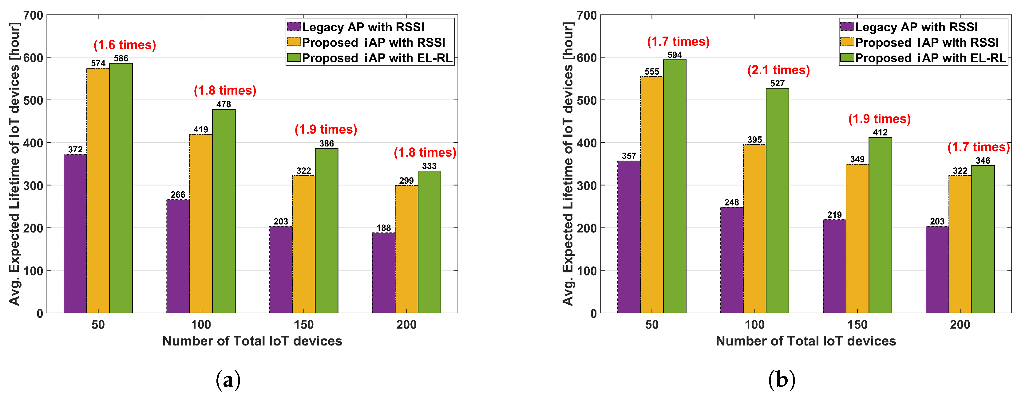
Figure 13 presents the expected lifespan of an IoT device, under the different distribution ratios between APs. In Case 2 of the 1:9:9 distribution ratio between APs, the expected lifespan of an IoT device is shown in
Figure 13a. The ‘proposed iAP with EL-RL’ model can significantly enhance the expected lifespan, with an improvement ranging from
times to
times roughly when compared to the ‘legacy AP with RSSI’ model. Furthermore,
Figure 13b displays the expected lifespan of an IoT device according to Case 3 of the 1:10:3 distribution ratio between APs. The ‘proposed iAP with EL-RL’ model offers an even more significant improvement in the expected lifespan, roughly ranging from
times to
times when compared to the legacy AP model. From this, it can be seen that the ‘proposed iAP with EL-RL’ model shows better energy-saving performance as the unbalanced load situation deepens. As such, the increased expected lifespan of IoT devices using the ‘proposed iAP with EL-RL’ model can be of great help in providing various IoT services by solving the problem of frequent battery replacement.
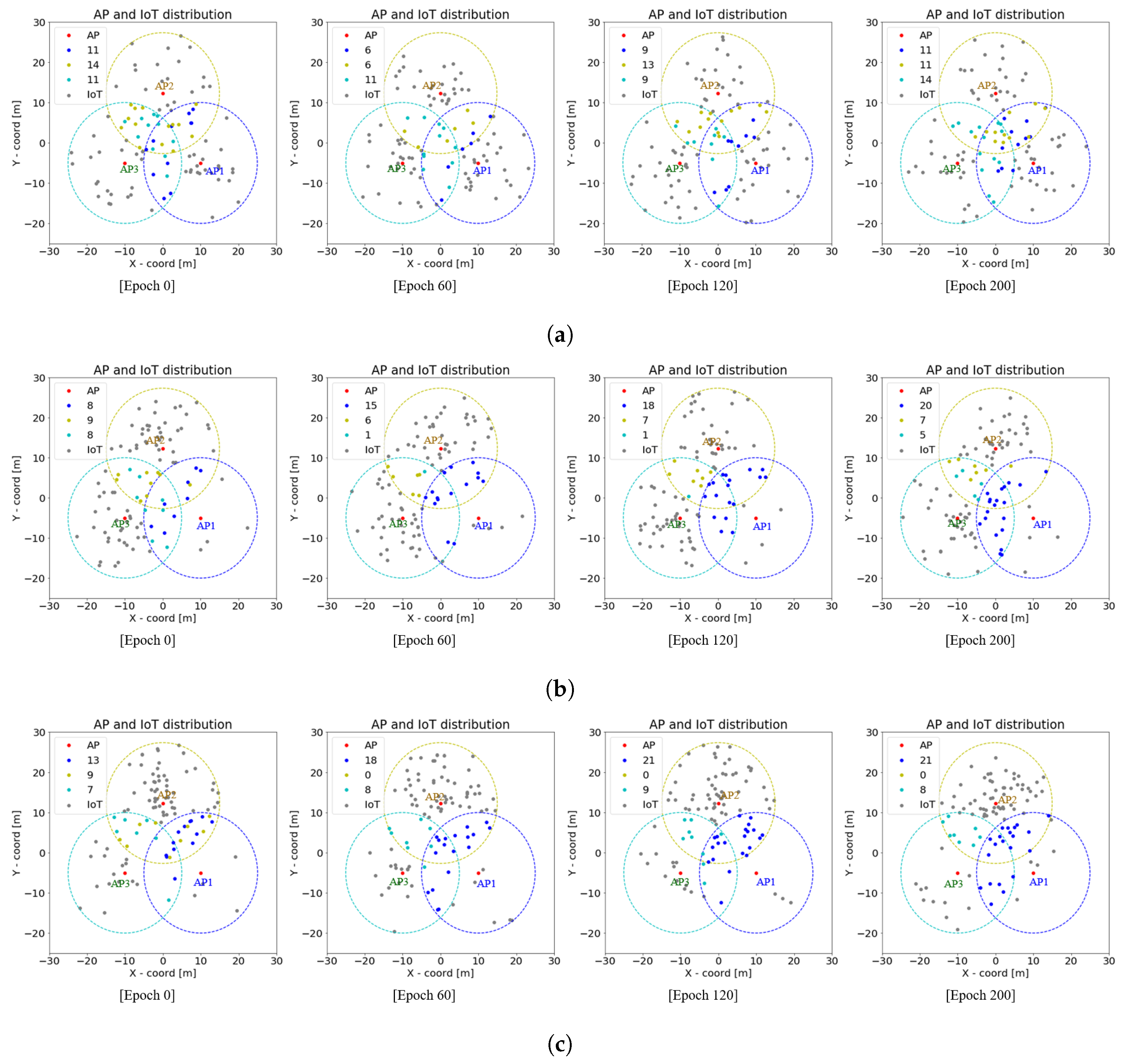
The generalization of IoT device location (i.e., the location of each IoT device has continuously changed as epoch increased) in the EL-RL model is demonstrated in
Figure 14 under three cases, each with a total of 100 devices and different distribution ratios between APs. In Case 1 where the distribution ratio is 1:1:1,
Figure 14a displays the location generalization. Case 2 with a distribution ratio of 1:9:9 is presented in
Figure 14b. Finally,
Figure 14c illustrates Case 3 where the distribution ratio is 1:10:3. As the epoch progresses, the IoT devices located at the overlapping section tended to select the AP connected with a smaller number of IoT devices to maintain stable load balancing in terms of energy efficiency and latency. Therefore, regardless of the distribution of IoT devices, the proposed EL-RL model can be stably trained under the generalization of IoT device location, and improve the energy efficiency and latency performance of IoT devices.
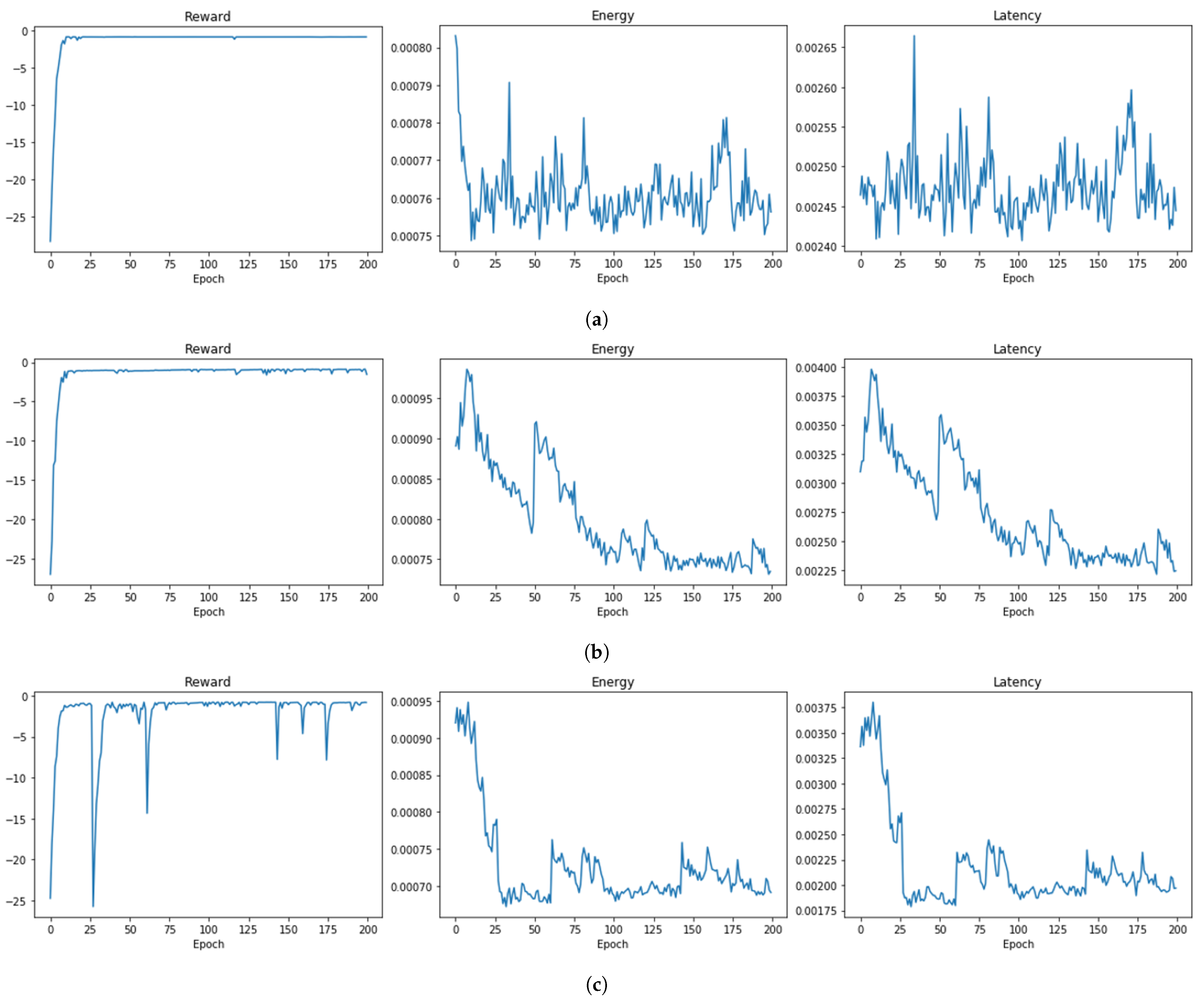
The convergence analysis of the EL-RL model is demonstrated in
Figure 15 under three different distribution ratios between APs, in order to examine its performance in various scenarios.
Figure 15a depicts the convergence behavior of the model when the distribution ratio is 1:1:1. The reward of the EL-RL model quickly and efficiently converges after approximately 25 epochs of training, while the energy consumption and latency also gradually converge as the epochs progress. Similarly, the convergence behavior of the EL-RL model is presented in
Figure 15b when the distribution ratio is 1:9:9. As observed in the previous case, the reward, energy consumption, and latency of the EL-RL model converge efficiently after approximately 25 epochs of training. Finally,
Figure 15c illustrates the convergence behavior of the EL-RL model when the distribution ratio is 1:10:3. The reward of the model gradually converges as the epochs progress, indicating that the reinforcement learning was successful. Although the reward changes rapidly in some cases, the range of change decreases as the learning progresses and ultimately converges. Additionally, the energy consumption and latency of the EL-RL model also converge as the epochs progress.
To address the training and inference time of the EL-RL model, we provide comprehensive information in
Table 4, which summarizes the average training time per epoch and the average inference time per input instance. The simulations were conducted on a computer system with a 64-bit Intel Core i7-800 CPU, and 16 GB of RAM. The simulation results reflect the duration required for training the EL-RL model and the inference time for making AP selections across different cases. It is noteworthy that the average training time per epoch increases with a higher number of MTs. Nevertheless, the overall training duration remains within 25 epochs, equivalent to less than 10 min. Furthermore, the training and inference procedures can be decoupled. The iAP operates using the most recently updated EL-RL model, which is redistributed to the iAPs when the model is updated at the iAP controller with an accumulated training dataset. This approach enables dynamic and iterative training, enhancing the model’s effectiveness over time. With an average inference time below
milliseconds, the EL-RL model has a minimal impact on the overall time required for establishing connections, typically measured in seconds [
28]. Therefore, the EL-RL model demonstrates its feasibility for real-world AP selection scenarios without significantly increasing connection setup delays. Finally, while the training and inference of the EL-RL model primarily utilize the CPU, incorporating GPU acceleration can further reduce processing time in both the training and inference stages.


