
Energy-Efficient Algorithms for Path Coverage in Sensor Networks

1
School of Computer Science and Engineering, Changsha University, Changsha 410022, China
2
Department of Computer Science and Software Engineering, Swinburne University of Technology, Hawthorn 3122, Australia
*
Author to whom correspondence should be addressed.
Sensors 2023, 23(11), 5026; https://doi.org/10.3390/s23115026
Submission received: 13 April 2023
/
Revised: 14 May 2023
/
Accepted: 23 May 2023
/
Published: 24 May 2023
(This article belongs to the Topic Wireless Sensor Networks)
Abstract
:Path coverage attracts many interests in some scenarios, such as object tracing in sensor networks. However, the problem of how to conserve the constrained energy of sensors is rarely considered in existing research. This paper studies two problems in the energy conservation of sensor networks that have not been addressed before. The first problem is called the least movement of nodes on path coverage. It first proves the problem as NP-hard, and then uses curve disjunction to separate each path into some discrete points, and ultimately moves nodes to new positions under some heuristic regulations. The utilized curve disjunction technique makes the proposed mechanism unrestricted by the linear path. The second problem is called the largest lifetime on path coverage. It first separates all nodes into independent partitions by utilizing the method of largest weighted bipartite matching, and then schedules these partitions to cover all paths in the network by turns. We eventually analyze the energy cost of the two proposed mechanisms, and evaluate the effects of some parameters on performance through extensive experiments, respectively.
1. Introduction
Wireless sensor networks (WSNs) are generally regarded as a type of smart network which consists of multiple nodes with limited capabilities on energy, computation, and storage [1]. In certain popular scenarios of these networks (e.g., target tracing), people have a great interest in guarding an object’s moving trail. This type of problem is called path coverage [2,3]. For nodes that are normally deployed at some sparse regions at random, a portion of them need to be moved to cover the path of the target, and minimizing the total moving distance of nodes should be considered seriously in resource-constrained networks [4]. Moreover, it is usually feasible to schedule these intensively deployed nodes for monitoring in some efficient ways to extend the life cycle of the network [5].
On minimizing the movements of nodes in sensor networks, some solutions have been presented for target coverage rather than for path coverage. Considering this, we propose a heuristic algorithm for minimizing the movements of nodes in sensor networks for path coverage for the first time in the heuristic algorithm; each path is divided into some discrete points by utilizing the curve disjunction technique. After finding out all redundant sensors and paths, sensors are then moved gradually to cover the given path under a set of regulations. As a result, path coverage can be achieved with the fewest movements of sensors.
On maximizing the lifetime of sensor networks, plenty of algorithms have been proposed, but most of them mainly focus on scenarios of point coverage and region coverage, rather than on those of path coverage. Therefore, we propose another heuristic algorithm on path coverage with the largest monitoring lifetime, which suits common sensor networks. Nodes are first divided into groups that can cover the path independently in the algorithm. Then, the largest weighted bipartite matching is utilized to schedule the nodes in each group. As a result, maximizing the lifetime of the network can be achieved.
The main contributions of this paper can be summarized as follows:
First, the problem of path coverage with the fewest movements of sensors is proved to be NP-hard, and then a new algorithm is proposed. The adopted curve disjunction technique overcomes the limitations of the linear path, which is a challenge in most of the existing schemes. Additionally, the effects of some parameters on moving distance are evaluated through further simulations.
Second, we present a heuristic algorithm for the problem of maximizing the lifetime of sensor networks on path coverage. In the experiments, we inspect not only the relationship between the number of nodes and lifetime of coverage, but also the relationship between the initial battery level and lifetime of coverage.
The rest of the paper is organized as follows. Related works on coverage in sensor networks are surveyed in Section 2. The algorithm on path coverage with the fewest movements in sensor networks is presented In Section 3, followed by Section 4, which presents the details of the largest lifetime of path coverage. Finally, Section 5 concludes the whole work.
2. Related Work
In recent years, some works have been presented to cope with the moving problems of sensors [5,6,7,8,9]. Liao et al. [5] gave a solution for the Mobile Nodes Deploying problem (MND) by decomposing it into two sub-steps. The first is the Target Coverage problem (TCP), and the second is the Network Connectivity problem (NCP). The named TCP problem concerns, supposing there exist m objects and n randomly located nodes, moving nodes to cover all objects with the least distance. It proved the NP-hardness of TCP, then solved TCP and NCP one by one, and finally addressed the MND problem through the combination of their solutions. Hefeeda et al. [6] proposed an approximated algorithm for k-coverage in intensively deployed sensor networks. Without considering the mobility of sensors, Zhang et al. [7] proposed a probabilistic mechanism. However, due to the fact that each node only works for another one that is out of service, the largest moving distance of each node is restricted. Attea et al. [8] modeled the Minimum Set Covering Problem (MSCP) to move sensors that can achieve energy-efficient coverage. Han et al. [9] proved that finding the largest number of crossed barriers is NP-hard, and presented a heuristic algorithm called MSPA based on a multi-round shortest path to solve the problem.
For maximizing the lifetime of sensor networks, many algorithms have been presented in recent years [7,10,11,12,13,14,15,16,17,18]. Dhawan et al. [10] proposed a mechanism to prolong the lifetime of the network by constructing the Lifetime dependency Graph (LG) to select a subset of sensors that can cover the target. Mini et al. [11] utilized the artificial bee colony algorithm and particle swarm optimization to schedule sensors to achieve the theoretical upper bound of a network’s lifetime. Abrams et al. [12] proved the problem of maximizing sensor network lifetime to be NP-Complete and presented a heuristic mechanism to solve it. Based on the method of separating nodes into the largest quantity of disjoint collections, Cardei et al. [13] proposed a scheme to extend networks’ monitoring lifetime. In the case of bounding the density of targets, Lu et al. [14] presented a PTAS mechanism to prolong the monitoring lifetime of the network and verified that, even in specialized conditions for nodes possessing the same sensing range and transmission range, the problem of scheduling nodes aimed to maximized lifetime belongs to NP-hard. Pointing to the scenario where nodes form a barrier to trace moving objects, Zhang et al. [7] provided an approximated algorithm for path coverage without considering energy optimization. Gu et al. [15] had a joint consideration of energy efficient routing and sleep scheduling, and mathematically formulated the lifetime maximization problem under multiple constraints (i.e., routing, end-to-end delay bounds, sleep scheduling, the energy consumption of transmission, receiving and listening, etc.). Considering that the formulated problem is a mixed integer non-linear programming (MINLP) problem and NP-hard to solve, they relaxed it into a linear programming (LP) problem and solved the relaxed problem for the upper bound. Weng et al. [16] proposed an Efficient k-Barrier Construction Mechanism (EBCM), aiming to schedule the sleep-wake time of all the constructed barriers to achieve energy balance. Yoon et al. [17] derived the upper and lower bounds on the coverage of a 2-D deployment of static sensors, and then used these bounds in constructing a method of estimating the coverage of deployment by assuming that there are only pair-wise intersections between the disks representing the range of each sensor. Ma et al. [18] proposed a hybrid strategy-improved butterfly optimization algorithm based on the elite-fusion and elite-oriented local mutation strategies.
As can be seen from the above, most of the existing works focus on point coverage or region coverage-related problems, while little attention has been paid to path coverage. This paper utilizes curve disjunction and largest weighted bipartite matching to achieve energy-efficient path coverage in sensor networks. The comparison of the main coverage algorithms is illustrated in Table 1.
3. Least Movement of Sensors on Path Coverage
3.1. Problem Description
We first define the problem under study and then prove its hardness in this section.
Definition 1.
Path coverage with least nodes’ movements Problem (noted as PCP). Supposing there exists a path P and a group of nodes belonging to collection S, move nodes to cover P with the least distance making the probability of each point in P being covered not less than d. The covering probability of a point is defined as follows in [3].
Definition 2.
Covering probability. The probability of node s covering object t is
When point j is covered by several nodes (s1, s2, …, sN), then Pj is the accumulative covering probability of s1, s2, …, and sN.
Note S(v) and P(u) as the collection of nodes covering point v, and the collection of points being covered by node u, respectively. Supposing Q is the collection of multiple disconnected points (p1, p2, …, pN), we note Mj(pi) as pi+j and Nj(pi) as pi−j, respectively.
Theorem 1.
PCP is an NP-hard problem.
Proof.
The proof is a deduction of TCP [5], which has already been verified as an NP-hard problem. First, supposing there exist m objects and n nodes in TCP, move nodes to cover all objects, making the total movement the least. Second, construct PCP as follows: sort all objects according to the x-axis, then connect all objects successively to form a path P, and finally, move nodes to cover P with the least distance.
In one case, suppose m new locations of nodes covering all objects with the fewest movements existed. The m discrete points mentioned above in P can be covered for the reason that P is constructed by m objects. As a result, m nodes in the new locations can cover P with the fewest movements in PCP.
In another case, assuming m new locations of nodes existed, which led to covering P with the fewest movements. It is easy to know that there are m discrete points in P being covered by these nodes. Here, m points are corresponding objects in TCP; thus, these new locations of nodes can cover all objects with the fewest movements in TCP.
Therefore, PCP is also NP-hard. □
3.2. The Least Movement Algorithm
The algorithm to solve PCP is divided into three steps: (1) separate the path into a partition of discrete points; (2) for nodes that do not cover any point in the path, move each of them to cover the closest point in P; and (3) move nodes to cover all discrete points with the least distance.
3.2.1. Path Disjunction
Path disjunction is to separate the given path P into multiple points in collection Q, which is implemented as follows: define a step-size threshold d, and in each run, fetch a point in P whose range is d far away from the former one according to the x-axis; carry this out continuously, until all of the n points are included in the collection Q finally. The corresponding pseudo-code is shown in Algorithm 1, which consumes time O(n).
| Algorithm 1: Curve disjunction |
| 1. Let step-size d be (big-coordinate − min-coordinate)/n; 2. Let the collection Q be NULL; 3. For i from 1 to n do 4. xi = (i − 1/2)d; 5. Insert the fetched point (h(xi), xi) into collection Q; 6. Return collection Q. |
3.2.2. Initial Movement
After deployment, we need to find out the nodes which are free of work and move each of them to cover at least one point, respectively. The aim of the initialized movement is illustrated below. Preset a group of nodes belonging to collection S and a group of points belonging to collection Q in path P; move each node that is not covering any point in P to cover the closest point in P. Here, we note the distance between the corresponding node and the point as R2. The pseudo-code is shown in Algorithm 2. As finding out the closest point in the path runs in O(n), judging every node needs time O(nm).
| Algorithm 2: Initializing movement |
| /* Input: points in collection Q with size n in path P, deployed node collection S with size m. Output: move S shortest such that for si in S, there exists pj in Q, where |si, pj| ≤ R2; */ 1. For i from 1 to m do 2. If |si, every point in Q| > R2, then 3. move si to its closest point pj such that |si, pj| = R2; 4. Return. |
3.2.3. Last Movement
After the initial movement, we need to move nodes further such that all discrete points in the path are covered. We first define the redundant node and redundant path, respectively, and then present the moving regulations.
Definition 3.
Redundant node. Assume that the covering probability of point j is not smaller than d in Q, i.e., Pj ≥ d; if the equation still works after taking node si out of S(j), then node si is called a redundant node.
In order to find out a redundant node of pi, we need to judge whether there is a redundant node: if point j has an initial covering probability not less than d, which becomes less than d after removing node s, then s is not redundant. Further, we need to check if the redundant node is closest among all neighbors of i. The pseudo-code of finding a redundant node is listed in Algorithm 3, which runs in time O(nm2).
| Algorithm 3: Find-redundant-nodes |
| /* Input: points collection Q with size n in P, nodes collection S with size m, point i. Output: the closest redundant node in S(i) to N(pos(i)).*/ 1. For (1≤ i ≤ n) & (Pi ≥ d), then 2. If Pi < d after moving s, then 3. Return Ø; 4. If orient = left, then 5. Set N(pos(i)) as Mj(pi) 6. Else if orient = right, then 7. Set N(pos(i)) as Nj(pi) 8. Else if orient = self 9. Set N(pos(i)) as i; 10. Take i out of Q; 11. If exist a closest redundant node s to N(pos(i)), then 12. Insert i into Q; 13. Return s. |
Definition 4.
Redundant path. For points p1, …, pi, assume the covering probability of p1 is less than d, and there are no redundant nodes in p2, p3, …, and pi−1, except that pi possesses a redundant node si. Find a partition of nodes s2, …, si, and move si to monitor pi−1, …; similarly, move s2 to monitor p1, such that all points have covering probability not smaller than d. Then, the path (p1, pi) is redundant.
We then present the heuristic regulations to move nodes.
Regulation 1.
To a point pj, whose covering probability is smaller than d, examine all redundant nodes in collection S(pj) and move the closest one to guarantee the probability of covering pj is not smaller than d.
Regulation 2.
Given path (pi, pk) and a redundant node in S(pj), if j = i − 1, we move the closest redundant node to guarantee pj is not smaller than d; otherwise, we move the closest redundant node of pj−1 to guarantee pj−1 not smaller than d.
When pj is smaller than d, we chase a redundant node in S(pj). If it works, Regulation 1 is applied to move nodes. Otherwise, we have to chase a redundant path. If it works, Regulation 2 is used.
The total algorithm for solving PCP is given in Algorithm 4. Combined with curve disjunction, initial movement, and last movement, PCP can be solved in O (n4m + n3m2).
| Algorithm 4: PCP solution |
| /* Input: points collection Q with size n in P, nodes collection S with size m. Output: move S shortest distance to cover P, or report failure.*/ 1. Rank all points in line with x-axis; 2. Compute covering probability of all elements in collection Q; 3. Let mv_len = 0; 4. Initializing node movement; /*Algorithm 2*/ 5. For (0 ≤ i ≤ n) & For (1 ≤ j ≤ n) 6. If exists redundant node s in S(Mi(pj)) or S(Ni(pj)), then 7. When (i = 0), move s to s0 according to Regulation 1; 8. mv_len = mv_len + |s0, s|; else 9. If s in S(Mi(pj)), then let orient be left 10. Else let orient be right. 11. If x0 in Mi(pj) or Ni(pj) possesses a redundant node; 12. Note path (pf, pf−1, …, p1); 13. For (r = f, r--, r ≥ 1) 14. If exists redundant node s in S(pr), then 15. When (r ≥ 2) then move node according to Regulation 2. 16. Else move s according to Regulation 1; 17. Move node to s0; add |s0, s| to mv_len. |
3.2.4. Simulations
To confirm the effectiveness of the proposed scheme, we establish the simulated platform using the Python and C++ languages. Due to the limitation of space, we only present results for the changing conditions of the total moving distance of nodes, according to variations of the number of discrete points in the path, parameters R1 and R2, respectively. The size of the monitoring region is 100 × 100 m2, where 120 nodes are located at random in it. Additionally, we use function y = 0.1 × (x − 10) × (x − 20) (0 < x < 100) to generate points in the path. The threshold of covering probability d is set as 0.5, and β is set as 0.5. The sensing radius R1 changes from 0 to 2.5 m, and R2 changes from 2.5 m to 5 m, respectively. We also observe the moving conditions of nodes. The results are averaged over 10 simulated topologies.
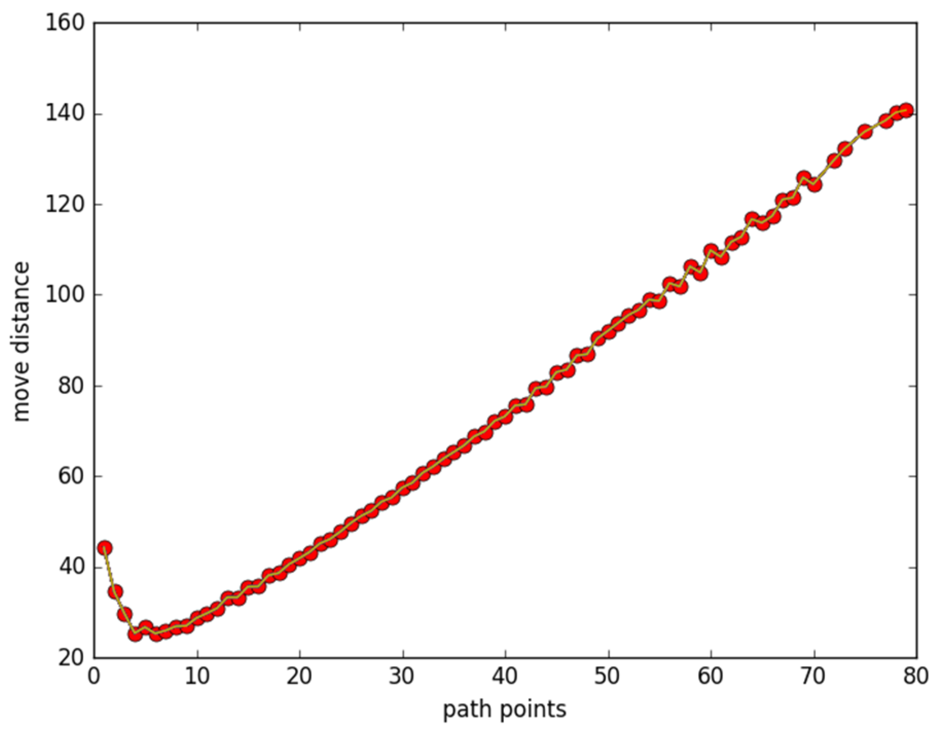
Figure 1 plots how the total moving distance changes as a function of the number of discrete points in the path, with 80 nodes located randomly in the area. Discrete points in the path are produced using the following function: y= 0.1(x − 20)(x − 10) (0 ≤ x ≤ 100). Other parameters are set as d = 0.5, R1 = 2.5, R2 = 5, and β = 0.5, respectively. As can be seen in Figure 1, there exists turning points in the curve on about five discrete points. At first, with few discrete points, all nodes have to move to their closest places. With the increase in the number of points, the moving distance decreases. However, as the number of points increased to some critical value (about eight here), more movements would be required to meet the covering expectations of all points.
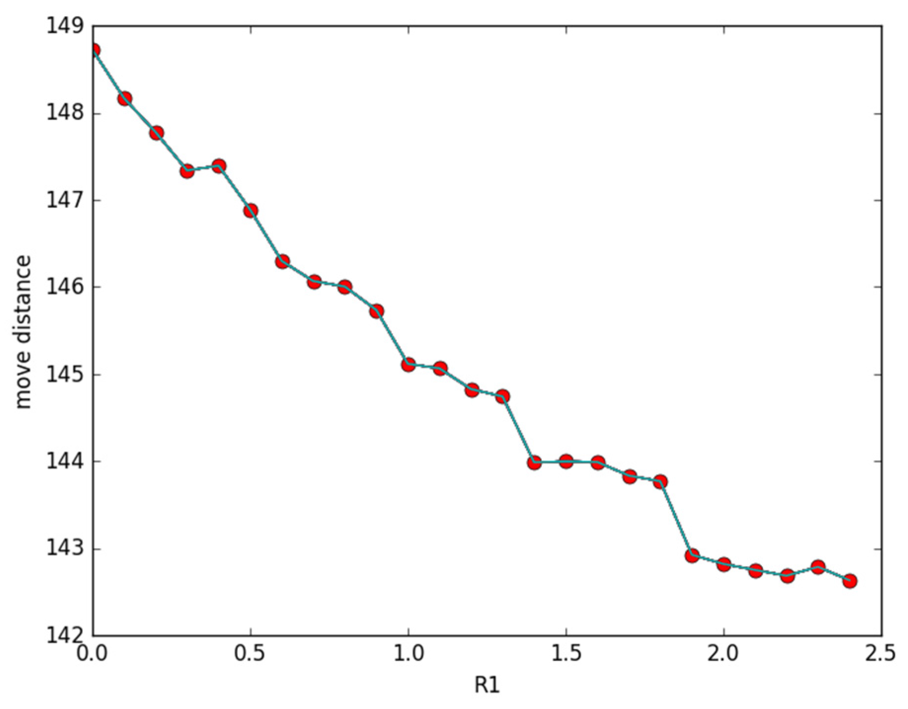
Figure 2 illustrates the changing conditions of the total moving distance according to variations in the sensing radius. We also use the same curve function, y, to generate 80 discrete points in the path, and then deploy 120 nodes randomly in the region. R1 ranges from 0 to 2.5 m, and the other parameters are set as d = 0.5, β = 0.5, and R2 = 5 m, respectively. It can be noticed from Figure 2 that moving distance decreases gradually in accordance with the increase in R1. This is because when R1 increases, the covering probability of all discrete points around it will become larger.
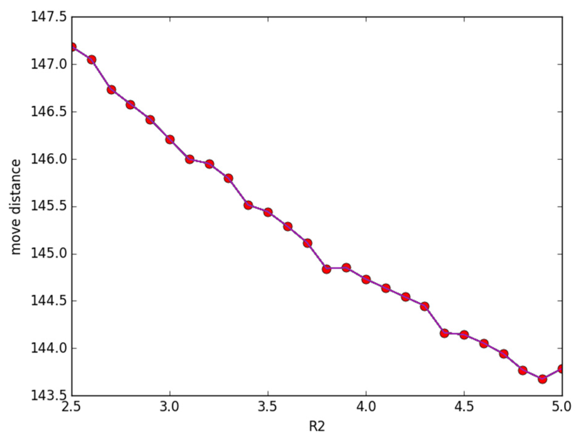
Figure 3 plots how the total moving distance changes according to R2. The parameters evaluating covering performance are set as R1 = 2.5, d = 0.5, and β = 0.5, respectively, while R2 changes from 2.5 m to 5 m. The other parameters are the same as in Figure 2. We observe that in Figure 3, with the increase of R2, the moving distance decreases. This phenomenon is caused by some discrete points being out of monitoring at the beginning while they are covered by nodes with the increase in R2.
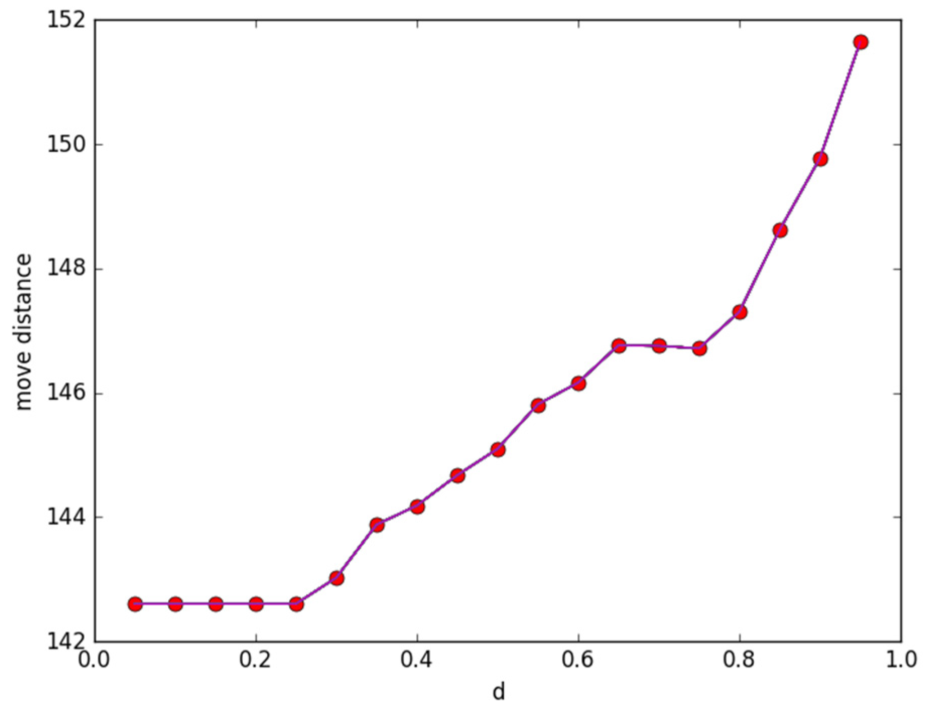
Figure 4 presents the changing condition of moving distance according to threshold d. In the initialized phase, we randomly produce 120 sensors in the monitoring area. Additionally, the same path function as in Figure 1 is taken to generate 80 discrete points. The covering probability threshold is ranged in (0.05, 0.95), and the other parameters are set as β = 0.5, R1 =2.5, and R2 = 5, respectively. We change the covering probability threshold d gradually. It can be observed from Figure 4 that, with the increase in d, the moving distance increases accordingly.
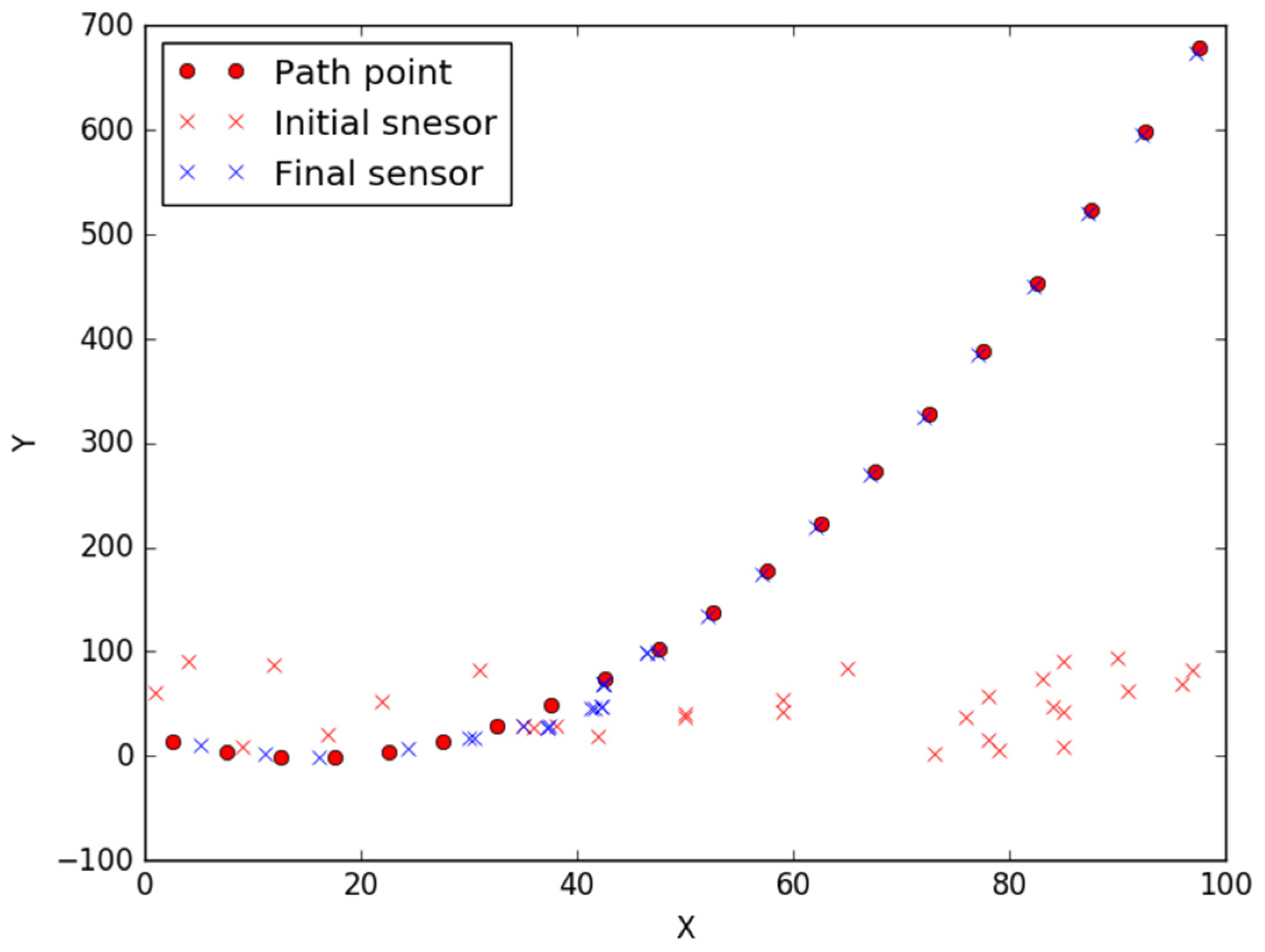
Figure 5 shows the conditions of node deployment and movement in order to cover all discrete points in the path. Twenty discrete points are generated through the function of y = 0.1 × (x − 20) × (x − 10) (0 ≤ x ≤ 100), and then 30 nodes are located randomly in the area of 100 × 100 m2. The other parameters are set as d = 0.5, β = 0.5, R1 = 2.5, and R2 = 5, respectively. We observe from the curve that nodes move efficiently to save energy.
4. Largest Path Coverage Lifetime
4.1. Problem Analysis
4.1.1. Marks
This section introduces the symbols that will be used in later aspects.
- E(s): The remaining battery level of node s, which is also called the lifetime of s;
- S(v): The collection of nodes that covered point v;
- C(s): The collection of points within the covering region of node s.
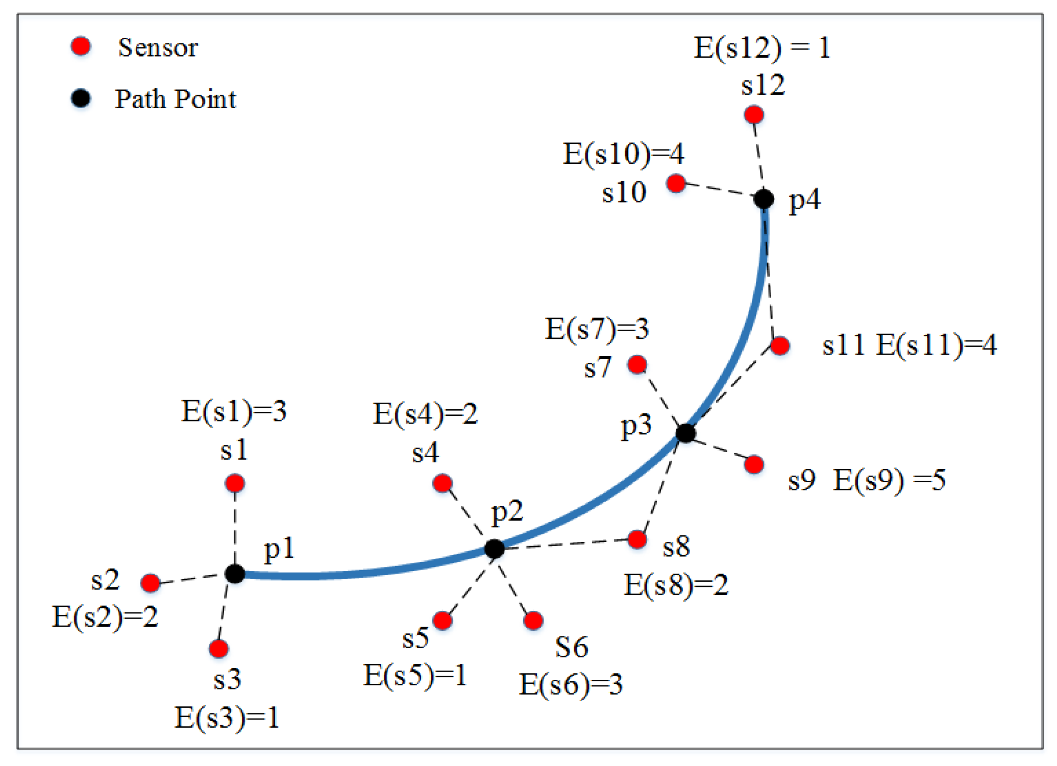
As illustrated in the network in Figure 6, twelve nodes and four points are located in the area. According to the definitions, here we have E(s1) = 3, S(p1) = {s1, s2, s3}, and C(s8) = {p2, p3}.
4.1.2. Preliminaries
Definition 5.
Coverage-weighted bipartite graph. In a sensor network, the graph is built as follows: B = (V1, V2, E). Here, the set V1 is composed of vertices representing the corresponding nodes, and the collection V2 contains vertices marking the corresponding points. When v belongs to collection C(u), the tuple (u, v) is treated as an edge in E. The value of (u, v) represents the residual battery level of node u.
For nodes that are usually deployed densely, only parts of them need to be activated to cover all points in some fixed time; the others turn to sleep mode.
Definition 6.
Path coverage lifetime. It is defined as the period of time that starts at all points being covered completely by nodes, and ends at any point where all the nodes cannot be covered.
Definition 7.
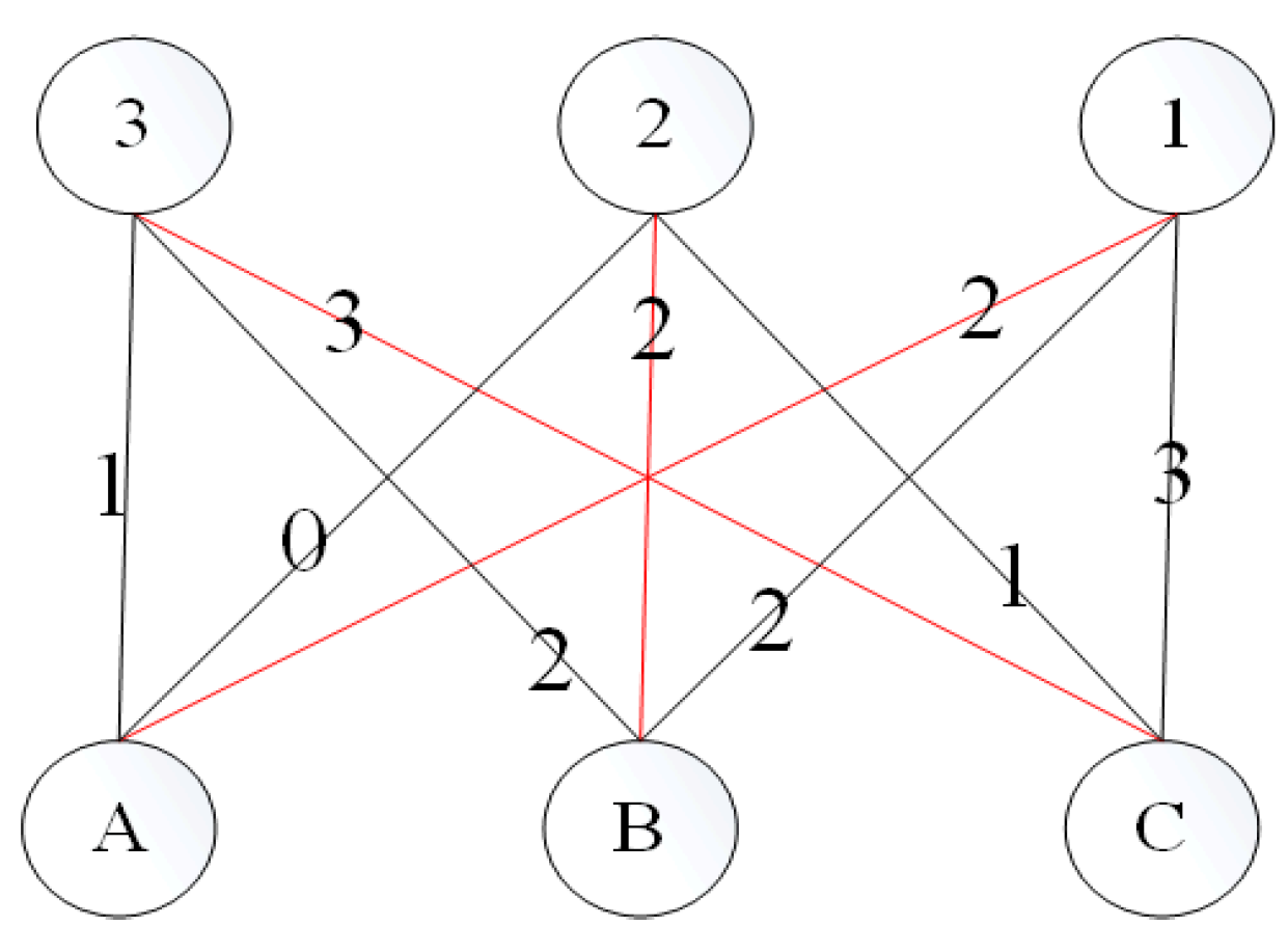
Largest Weighted bipartite Match (noted as LWM in later chapters). A match is defined in a graph G as a collection of edges that are vertex-disjoint. For a weighted bipartite graph, if the summation of values of all edges is the largest among all situations, then the weighted bipartite graph value is called LRM. As in Figure 7, A,B,C and 1,2,3 within each circle represents six different vertices, while the other numbers represent the value of each edge, respectively. Here LRM is {(1, A), (2, B), (3, C)}, with the summation of values even.
4.1.3. Problem Description
Considering the following problem: assuming multiple nodes are located randomly along a path, we first separate them into h partitions, then seek a way to schedule them in turn for path coverage with the largest monitoring lifetime (noted as PCLL). As in Figure 5, two partitions of nodes are formed: T1 = {s1, s4, s7, s10} and T2 = {s2, s3, s5, s6, s8, s9, s11, s12}, respectively. T1 is first used to monitor the path, and then T2 is taken to execute the task after some nodes in T1 exhaust their energy. T1 and T2 might not be the best partitioning solution; thus, some heuristic regulations are necessary for seeking a nearly optimal way.
In order to solve the PCLL problem, we decompose it into four steps: (1) separate the path into some discrete points, and divide all nodes into h partitions, respectively; (2) for the partitions that cannot cover all points completely, combine some of them to cover all points; (3) schedule all partitions to maximize the covering lifetime; and (4) schedule nodes within each partition to extensively maximize the covering lifetime. The mechanism for solving PCLL is formed through the combination of solutions of the above steps.
4.2. Largest Path Coverage Lifetime Algorithm
4.2.1. Nodes Partitioning
Before the phase of node partitioning, we also use Algorithm 1 to make the path discrete, which is omitted here.
For a fixed path P and a collection of distributed nodes S, h partitions of nodes T1, T2, …, and Th are found, each of which can cover some points on path P. The collection S(p) of point p is separated into k partitions randomly, and each covers some number of points. The nodes partitioning solution is given in Algorithm 5. It loops h × n times since some points from each S(pj) are removed randomly in a round; thus, the algorithm consumes a total of O(hnm) energy.
| Algorithm 5: Nodes-partition (S, Q) |
| /* Input: deploy nodes collection S = {v1, v2, …, vn}, and points collection Q = {p1,…,pm} in P. Output: partitions collection of nodes. */ 1. Note S(pi) be the collection of nodes covering point pi; 2. Note T1, T2, …, Th be collection of node partitions; 3. S1 = Ø; 4. For (1 ≤ i ≤ h) & (1 ≤ j ≤ m) 5. randomly pitch a subset S0 of S(pj); 6. Ti = Ti + (S0 − S1); 7. S(pj) = S(pj) − (S′ − S1); 8. S1 = S1 + (S0 − S1); 9. Return T1, T2, …, Th. |
4.2.2. Combine Partitions
After obtaining h partitions of nodes, a partition combination is needed to achieve the object that each new partition can cover all points completely. The problem is defined as follows: given h partitions of nodes T1, T2, …, Th and a collection of points Q, produce new collections of nodes W1, W2, …, Wr (r ≤ h), making each collection Wi cover all points in collection Q.
The solution is as follows: (1) first, arrange all partitions according to the number of points covered, and then take the first partition Ti out of them; if Ti can cover all the points, it is merged into collection Wi and then removed from the partitions; (2) otherwise, we put Ti into collection Wi and then fetch the next partition Ti+1. (3) In the case where Ti+1 is able to cover the point left by Wi, it is merged into Wi, too; execute the above procedure continuously, stopping only when all points are covered by Wi or all partitions are handled completely. (4) In the case that some points are left by Wi, we check if there is a collection Wj which is able to cover all points, and all remained partitions will be merged in a new collection Wj with the combination of Wi. In Algorithm 6, computing the number of points being covered by nodes takes O(hnm), sorting partitions takes O(hlogh), and combining partitions takes O(h2). Thus, the algorithm totally consumes O(hnm + h2).
| Algorithm 6: Combine-partition (T, Q) |
| /* Input: collection T = {T1, T2,…, Th} of node partitions, collection Q = {p1,…,pm} of points in P Output: new partition collections W1, W2, …, Wr (r ≤ h), each covers all points in collection Q. */ 1. Arrange T by quantity of covered points by Ti, denoted by T = {T1, T2, …, Th}. 2. r = 1; T0 = T; S0 = Q; 3. If (r ≤ h) 4. Set Wr be zero, j be one, respectively; 5. If (T0 is not null) & (S0 is not null) & (j ≤ h) & (|C(Tj) − (Q − S0)| ≤ 0) 6. j++; Wr = Wr + { Tj }; T0 = T0 − Tj; S0 = S0 − C(Tj); j++; 7. If (S0 is null collection) 8. r++; else if (r ≤ 1) 9. Return zero; else 10. Merge all collections in T0 with Wr − 1; Merge all collections in Wr with Wr − 1; r--; 11. Return W1, …, Wr. |
4.2.3. Partition Schedule
The partition schedule can be defined as follows: given some partitions of nodes, schedule them to achieve the largest lifetime of path coverage. It is obvious that the largest lifetime can be achieved by executing each partition once. The algorithm is given in Algorithm 7, which consumes time O(r).
| Algorithm 7: Partition schedule (W) |
| /* Input: partition collections W = {W1, W2, …, Wr} (r ≤ h), each covers all points in Q = {p1,…,pm}. Output: the schedule of collections in W */ 1. Calculate expected lifetime for each Wi; 2. For (1 ≤ i ≤ r) 3. Command nodes in collection Wi covering points in collection P; 4. Return. |
4.2.4. Intra-Schedule
Intra-scheduling aims to seek a method of making nodes in activating or sleeping mode, thus achieving the largest coverage time. To solve this, we first construct a coverage-weighted bipartite graph G and then seek an LRM in G. As a result, it is able to schedule nodes with the largest residual battery level. If they are not able to cover all points, we continue to construct the coverage-weighted bipartite graph G0 for those points left over, which stops when all points are covered, or the remaining nodes cannot cover all points. The pseudo-code is described in Algorithm 8. As illustrated, finding the largest weighted matching consumes (n2m); thus, the total time consumed is O (n2m2w), where w is the largest value.
| Algorithm 8: Intra-partition scheduling (Wi, Q) |
| /* Input: node collection Wi covering all points in collection Q = {p1,..,pm}. Output: schedule of nodes */ 1. While nodes in Wi cover all points in Q 2. Produce G = (V1,V2,E), where V1 denotes nodes set in Wi, and V2 denotes points set in Q; 3. Find a LRM (noted as M) in G; 4. For each vertex without matching in V2 5. Denote unmatched vertices set by V2′ in V2; 6. Induce a new sub-graph G0 from V1 and V2′; 7. Find a LRM in G0; 8. For element v in V2, note M(v) as the element in collection V1 matching some element of v in collection V2, and the one in M(v) with least battery be ver0; 9. For element v in collection V2, schedule M(v) to cover point v and point M(v), thus each element in collection Vi cost ver0 battery; 10. Delete elements in Wi out of service. 11. Return. |
4.3. Simulations
We use simulations to further evaluate the effect of the number of nodes on the largest path coverage lifetime. As there is only one existing work analyzing path coverage in specialized situations, it is unfeasible to compare the simulation results with former works. A given path is divided into ten discrete points, and then a group of sensors is deployed around these points. The points covered by each sensor are also continuous. Due to space limitations, we only consider the impacts of the following parameters, quantity of nodes, initial battery level, and sensing radius. For parameter setting, the path is separated into ten points, while the energy of each node is set to a random number in the interval [5,10]. We assume that each node can cover one to three discrete points. The results are averaged over 10 simulated topologies.
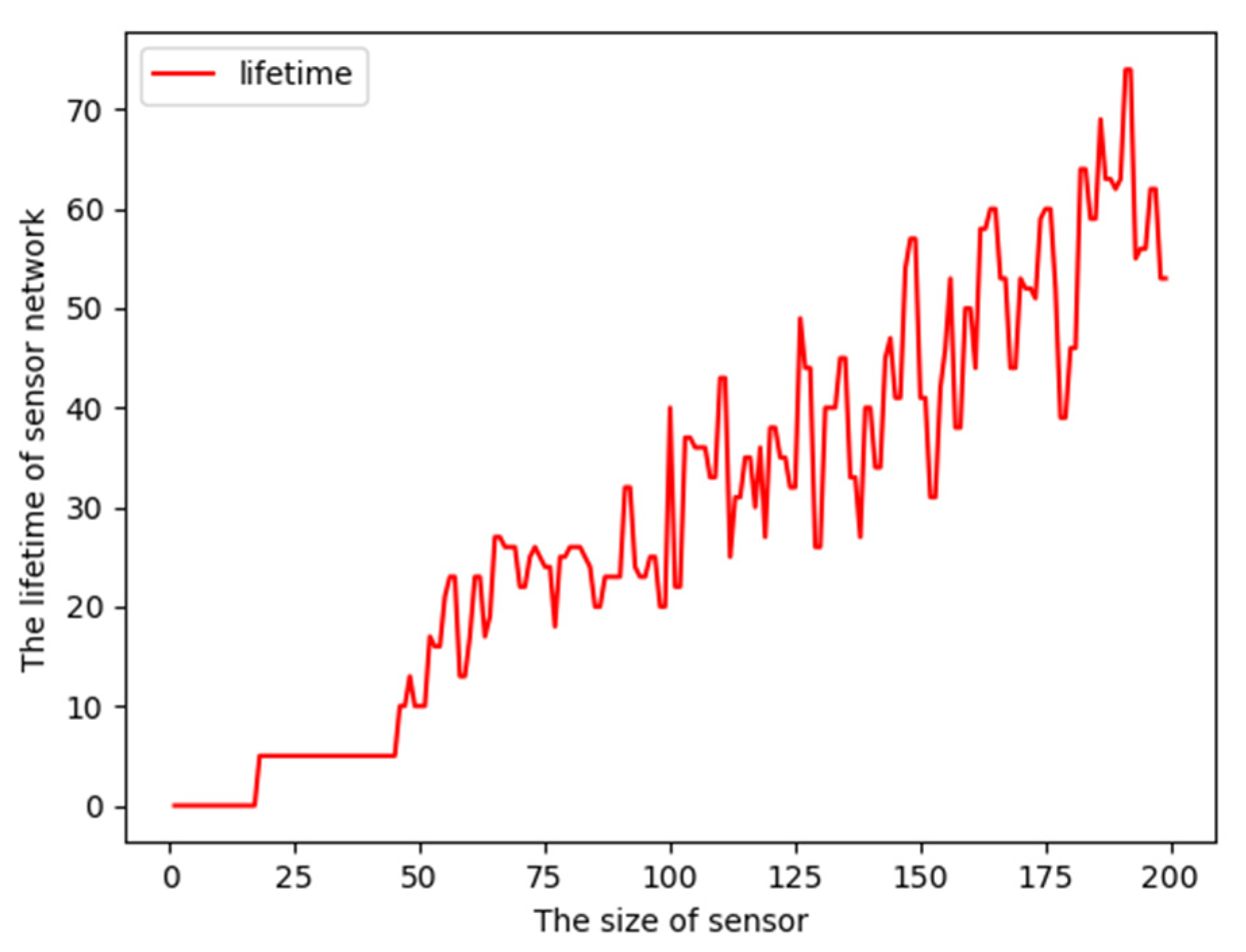
The lifetime function curve changing with the size of nodes is illustrated in Figure 8. From Figure 8, we know that with a small number of nodes, the path coverage lifetime is zero. This is because of the lack of enough nodes to cover all points. With the number of nodes increasing, the coverage lifetime increases gradually as more nodes are engaged to cover points.
The effect of the least initial battery level on the largest lifetime is given in Figure 9. Here, 200 nodes are located randomly around 10 discrete points in the path, and each node is equipped with the same battery initially. From Figure 9, we observe that the coverage lifetime also increases with the increase in the initial battery level of nodes, which enables nodes to monitor for a longer time.
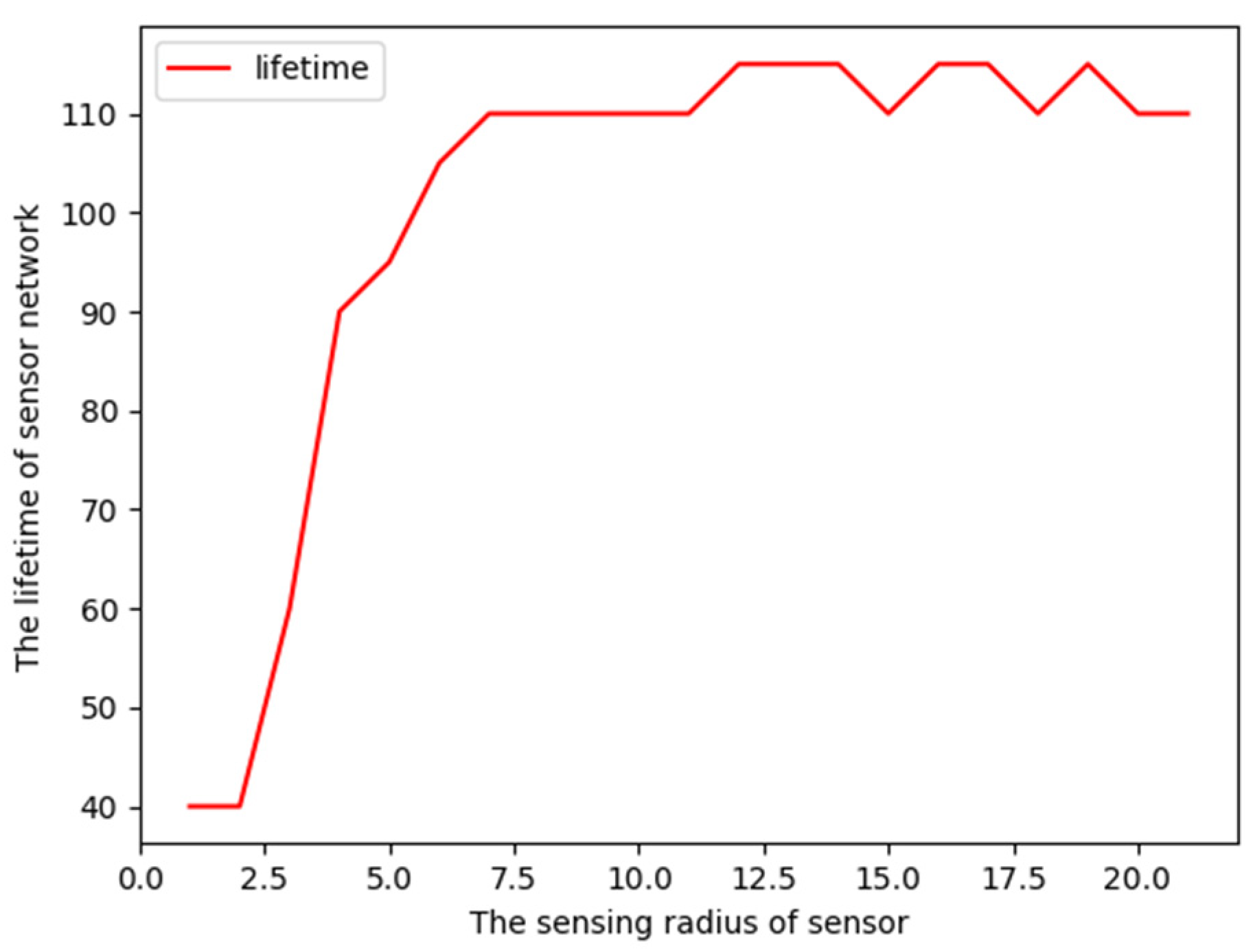
The changing condition of coverage lifetime with sensing radius is also investigated in Figure 10. The path is separated into 10 points, around which are located 200 nodes randomly, and each node is equipped with the same energy valued randomly in the interval [5,10]. From Figure 10, we see that the coverage lifetime is positively related to the sensing radius, i.e., the larger the sensing radius, the bigger the coverage lifetime. However, after the sensing radius increases to a certain threshold, the coverage lifetime does not increase any longer. This is because, in the situation where the sensing radius is equal to the threshold, the nodes can cover the entire region completely.
5. Conclusions
In this paper, we have presented algorithms for two path coverage problems that had not been considered before: path coverage with the fewest movements of nodes, and node scheduling for maximizing path coverage lifetime. We first separated each problem into several sub-problems and then solved them one by one, and the original problem was finally solved through the combination of all sub-problems. For the first problem, the NP-hardness of the problem was proved, and the fewest movements were achieved through finding redundant nodes and paths; while for the second one, the largest bipartite matching was utilized to schedule partitions of nodes for monitoring. Moreover, curve disjunction was used on both algorithms to divide the path into points, which enables the proposed algorithm to be expanded to common sensor networks. We also analyzed the time complexities of the proposed schemes, and further evaluated the performance through experiments. However, the performance of the proposed algorithms was only evaluated under the experimental circumstance; we yet need to carry out some further work in actual sensor network-related scenarios to validate their effectiveness, e.g., multimedia sensor networks, health care sensor networks, traffic monitoring networks, etc. Moreover, how the optimality of each sub-step in the proposed algorithms can be proved also needs some further investigation. As for future work, we plan to seek results for the above-mentioned limitations of the work.
Author Contributions
Conceptualization, Z.L.; methodology, Z.L.; software, Z.L.; validation, Z.L.; formal analysis, Z.L.; resources, Z.L.; data curation, Z.L.; writing—original draft preparation, Z.L.; writing—review and editing, W.Z.; visualization, Z.L.; supervision, W.Z.; project administration, Z.L.; funding acquisition, Z.L. All authors have read and agreed to the published version of the manuscript.
Funding
This research was funded by the National Natural Science Foundation of China, grant number 61502057.
Data Availability Statement
The experimental data was collected by the authors, and is not publicly available due to privacy.
Conflicts of Interest
The authors declare no conflict of interest.
References
- Tang, S.; Mao, X.; Li, X.Y. Optimal k-support coverage paths in wireless sensor networks. In Proceedings of the IEEE International Conference on Pervasive Computing & Communications, Washington, DC, USA, 9 March 2009. [Google Scholar]
- Bose, P.; Morin, B.; Stojmenovic, I. Routing with guaranteed delivery in ad hoc wireless networks. ACM J. Wirel. Netw. 1999, 7, 609–616. [Google Scholar] [CrossRef]
- Tan, R.; Xing, G.; Wang, J. Exploiting reactive mobility for collaborative target detection in wireless sensor networks. IEEE Trans. Mob. Comput. 2010, 9, 317–332. [Google Scholar] [CrossRef]
- Somasundara, A.; Ramamoorthy, A.; Srivastava, M. Mobile element scheduling with dynamic deadlines. IEEE Trans. Mob. Comput. 2007, 6, 395–410. [Google Scholar] [CrossRef]
- Liao, Z.; Wang, J.; Zhang, S. Minimizing movement for target coverage and network connectivity in mobile sensor networks. IEEE Trans. Parallel Distrib. Syst. 2015, 26, 1971–1983. [Google Scholar] [CrossRef]
- Hefeeda, M.; Bagheri, M. Randomized k-Coverage algorithms for dense sensor networks. In Proceedings of the International Conference on Computer Communications, Anchorage, AK, USA, 6 May 2007. [Google Scholar]
- Zhang, Y.; Huang, H.; Sun, P. Improving path-coverage for moving targets in wireless multimedia sensor networks. J. Commun. 2014, 9, 843–850. [Google Scholar] [CrossRef]
- Attea, B.A.; Hameed, S.M. A genetic algorithm for minimum set covering problem in reliable and efficient wireless sensor networks. Iraqi J. Sci. 2015, 55, 224–240. [Google Scholar]
- Han, R.S.; Wei, Y.; Li, Z. Achieving Crossed Strong Barrier Coverage in Wireless Sensor Network. Sensors 2018, 18, 534. [Google Scholar] [CrossRef] [PubMed]
- Dhawan, A. Maximum lifetime scheduling in wireless sensor networks. In Wireless Sensor Networks, Technology and Protocols; Intech: London, UK, 2012. [Google Scholar]
- Mini, S.; Udgata, S.K.; Sabat, S.L. Sensor deployment and scheduling for target coverage problem in wireless sensor networks. IEEE Nodes J. 2014, 14, 636–644. [Google Scholar] [CrossRef]
- Abrams, Z.E.; Ashish, G.; Serge, P. Set k-cover algorithms for energy efficient monitoring in wireless sensor networks. In Proceedings of the International Symposium on Information Processing in Sensor Networks, Berkeley, CA, USA, 27 April 2004. [Google Scholar]
- Cardei, M.; Du, D.Z. Improving wireless sensor network lifetime through power aware organization. Wirel. Netw. 2005, 11, 333–340. [Google Scholar] [CrossRef]
- Lu, Z.; Li, W.W.; Pan, M. Maximizing lifetime scheduling for target coverage and data collection in wireless sensor networks. IEEE Trans. Veh. Technol. 2015, 64, 714–727. [Google Scholar] [CrossRef]
- Gu, Y.; Pan, M.; Li, W. Maximizing the lifetime of delay-sensitive sensor networks via joint routing and sleep scheduling. In Proceedings of the IEEE International Conference on Computing, Networking and Communications, Honolulu, HI, USA, 15 January 2014. [Google Scholar]
- Weng, C.I.; Chang, C.Y.; Hsiao, C.Y. On-supporting energy balanced k-barrier coverage in wireless sensor networks. IEEE Access 2018, 99, 274–278. [Google Scholar] [CrossRef]
- Yoon, Y.; Kim, Y.H. Maximizing the coverage of sensor deployments using a memetic algorithm and fast coverage estimation. IEEE Trans. Cybern. 2021, 99, 6531–6542. [Google Scholar] [CrossRef] [PubMed]
- Ma, D.; Duan, Q. A hybrid-strategy-improved butterfly optimization algorithm applied to the node coverage problem of wireless sensor networks. Math. Biosci. Eng. 2022, 19, 3928–3952. [Google Scholar] [CrossRef] [PubMed]
Figure 1.
Moving distance changes with number of discrete points.

Figure 2.
Moving distance changes with R1.

Figure 3.
The change in R2 with the moving distance.

Figure 4.
The change in d with the moving distance.

Figure 5.
The movement of nodes.

Figure 6.
Path coverage in sensor network.

Figure 7.
Largest weighted matching.

Figure 8.
Lifetime changes with size of nodes.

Figure 9.
Lifetime changes with initial battery level.

Figure 10.
Lifetime changes with sensing radius.


Table 1.
Comparison of the coverage algorithms.
| Algorithms | Application Field | Object |
|---|---|---|
| MND [5] | point coverage | nodes movement |
| MTPCA [7] | point/region coverage | nodes movement |
| MSCP [8] | point/region coverage | nodes movement |
| MSPA [9] | barrier coverage | nodes movement |
| ABC [11] | point coverage | network lifetime |
| MC-MIP [13] | point coverage | network lifetime |
| MLCS [14] | point coverage | network lifetime |
| MSPA [16] | barrier coverage | network lifetime |
| HBOA [18] | point coverage | network lifetime |
| Our proposal | path coverage | nodes movement/network lifetime |
Disclaimer/Publisher’s Note: The statements, opinions and data contained in all publications are solely those of the individual author(s) and contributor(s) and not of MDPI and/or the editor(s). MDPI and/or the editor(s) disclaim responsibility for any injury to people or property resulting from any ideas, methods, instructions or products referred to in the content. |
© 2023 by the authors. Licensee MDPI, Basel, Switzerland. This article is an open access article distributed under the terms and conditions of the Creative Commons Attribution (CC BY) license (https://creativecommons.org/licenses/by/4.0/).
Share and Cite
MDPI and ACS Style
Liu, Z.; Zhou, W. Energy-Efficient Algorithms for Path Coverage in Sensor Networks. Sensors 2023, 23, 5026. https://doi.org/10.3390/s23115026
AMA Style
Liu Z, Zhou W. Energy-Efficient Algorithms for Path Coverage in Sensor Networks. Sensors. 2023; 23(11):5026. https://doi.org/10.3390/s23115026
Chicago/Turabian StyleLiu, Zhixiong, and Wei Zhou. 2023. "Energy-Efficient Algorithms for Path Coverage in Sensor Networks" Sensors 23, no. 11: 5026. https://doi.org/10.3390/s23115026
Note that from the first issue of 2016, this journal uses article numbers instead of page numbers. See further details here.