

Multi-Sensor Data Fusion and CNN-LSTM Model for Human Activity Recognition System


Abstract
:1. Introduction
2. Related Work
2.1. HAR Based on Single Sensor Data
2.2. HAR Based on Multi-Sensor Data Fusion
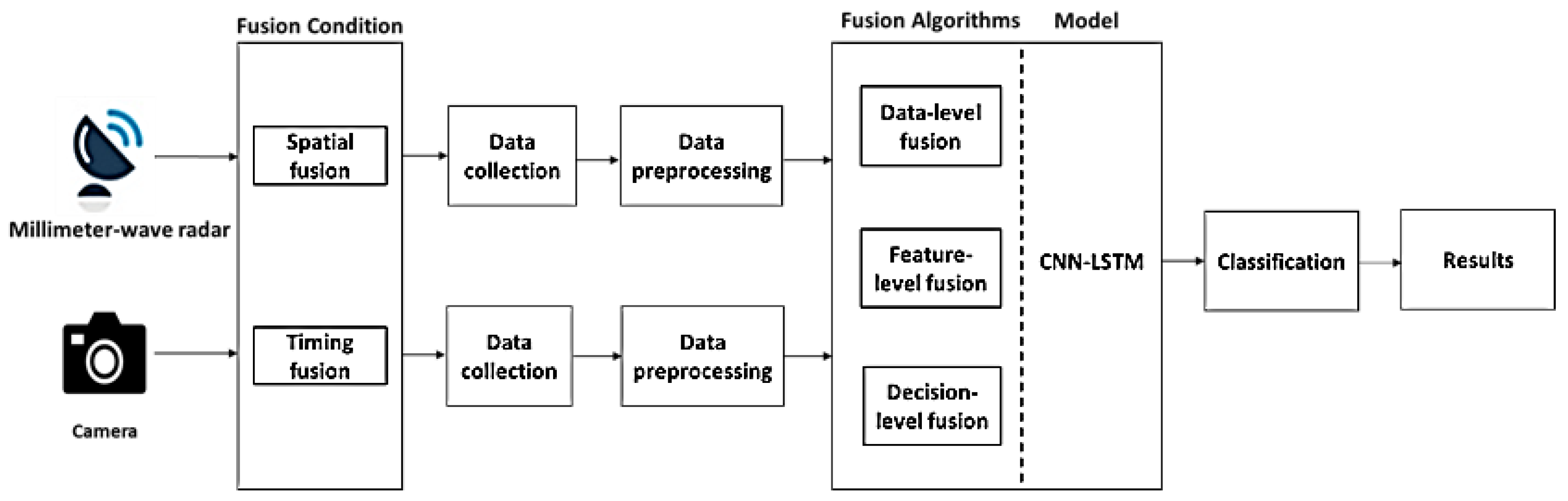
3. System Design
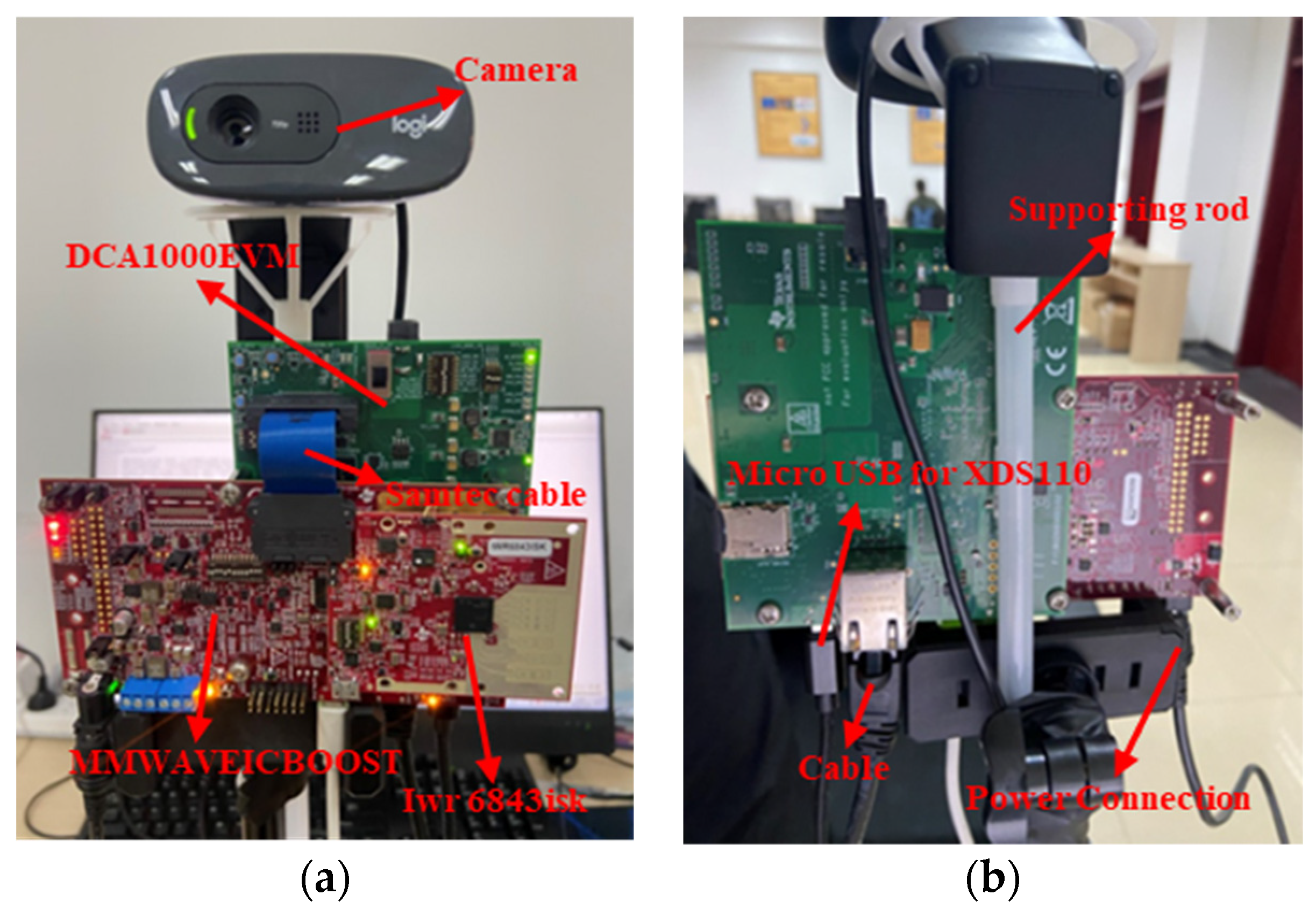
3.1. System Construction
- (1)
- Information about the IWR6843ISK
- (2)
- Information about DCA1000EVM
- (3)
- Information about MMWAVEICBOOST
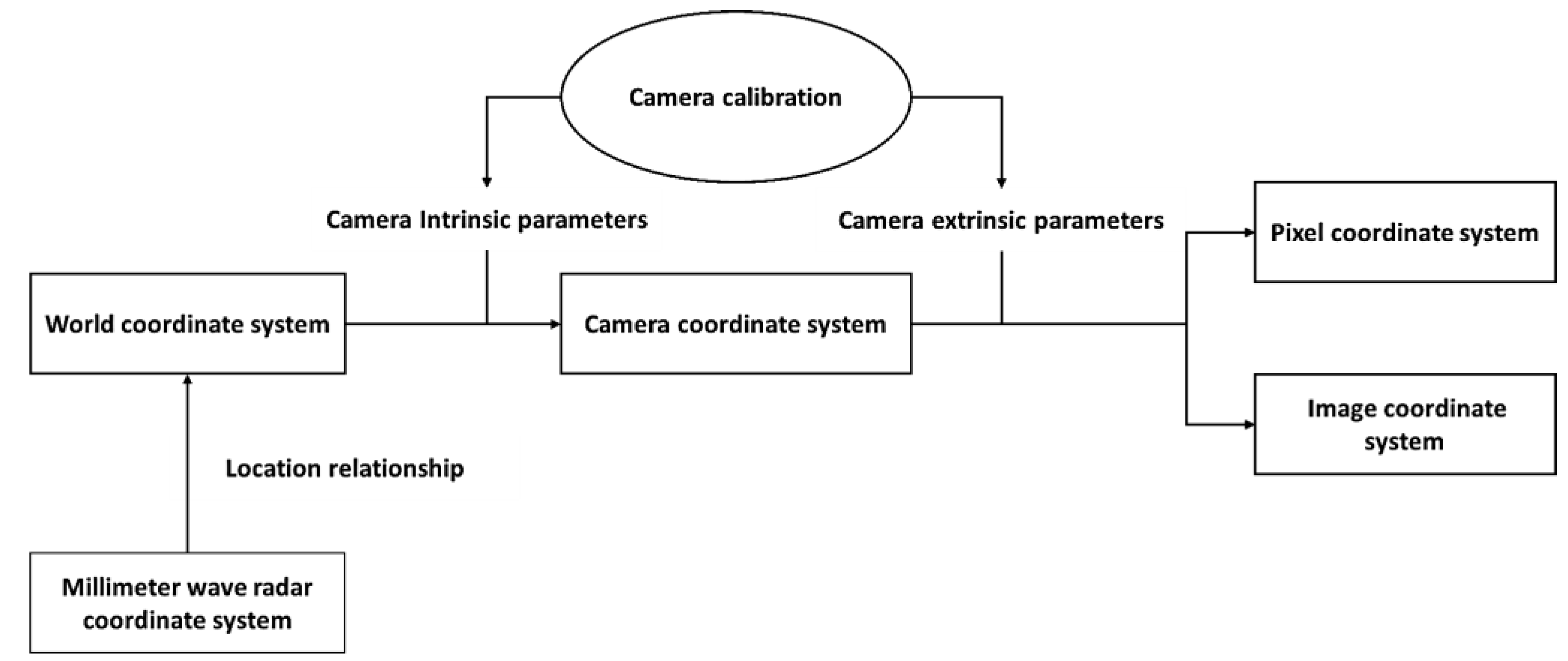
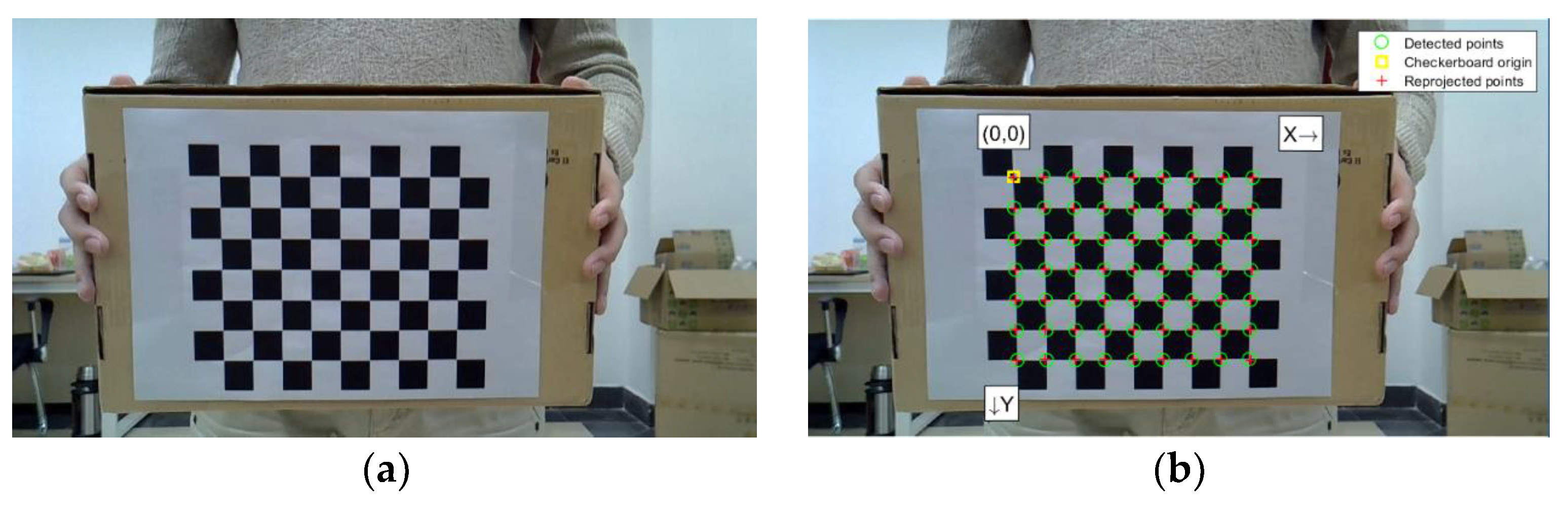
3.2. System Calibration
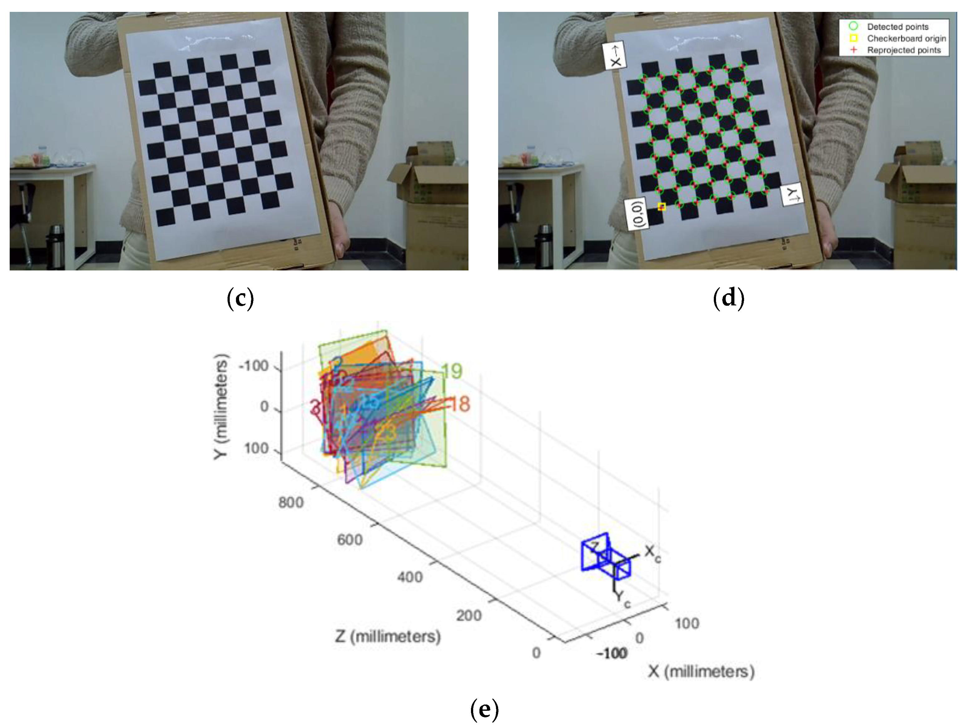
3.2.1. Spatial Calibration
- (1)
- Transformation of the camera coordinate system
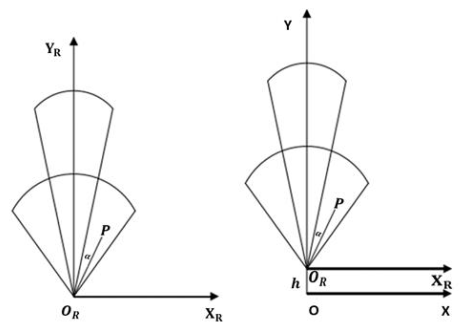
- (2)
- Transformation of the Millimeter Wave radar coordinate system
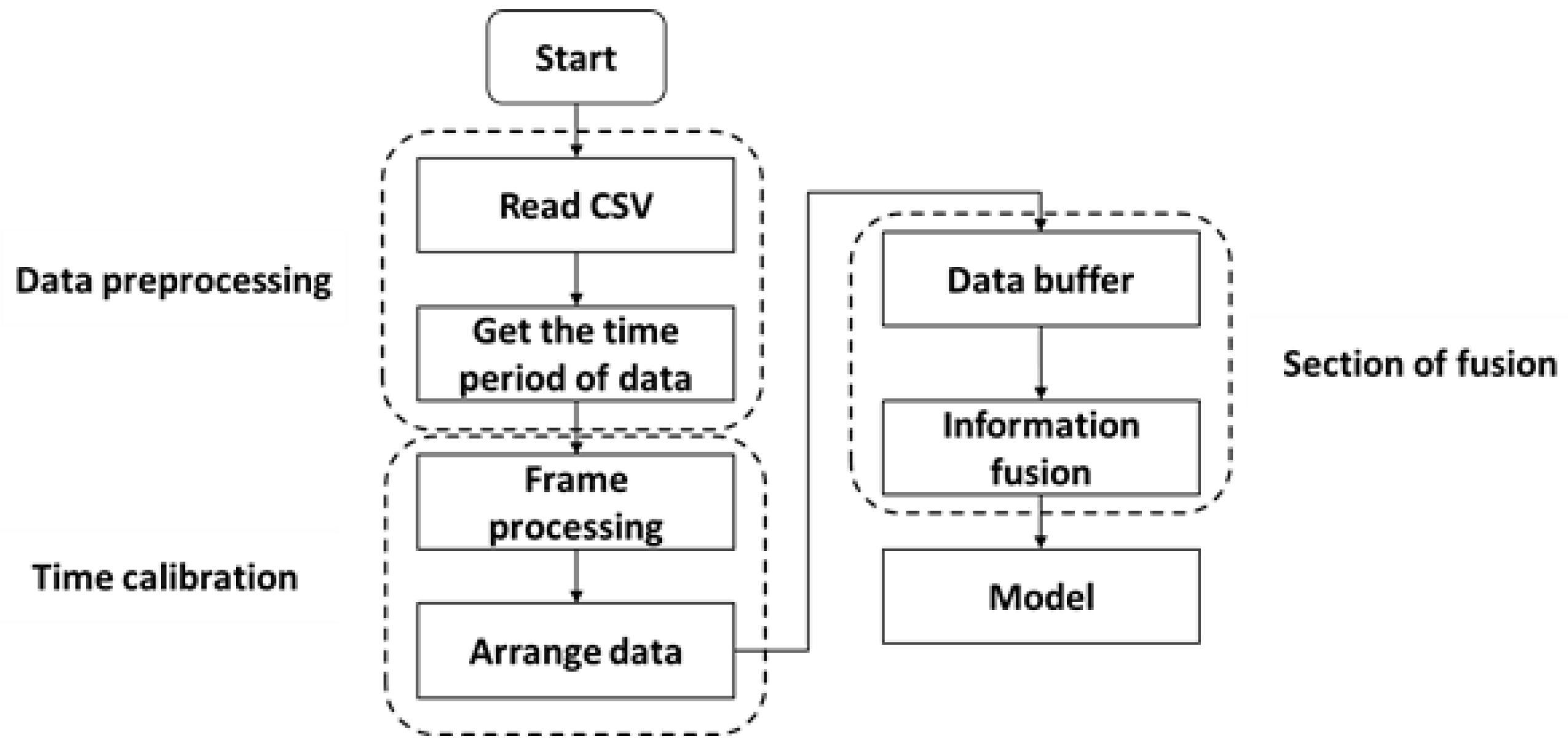
3.2.2. Time Calibration
- Reading the CSV data.
- Obtaining the timestamp of each sensor.
- Reducing the frame rate of the camera from 30 frames/s to 20 frames/s.
- Aligning the timestamp of the camera data with that of the radar data.
- Data fusion.
3.3. Data Preprocessing
3.3.1. Millimeter-Wave Radar Data
- (1)
- Time-frequency spectrogram
- (2)
- Range spectrogram
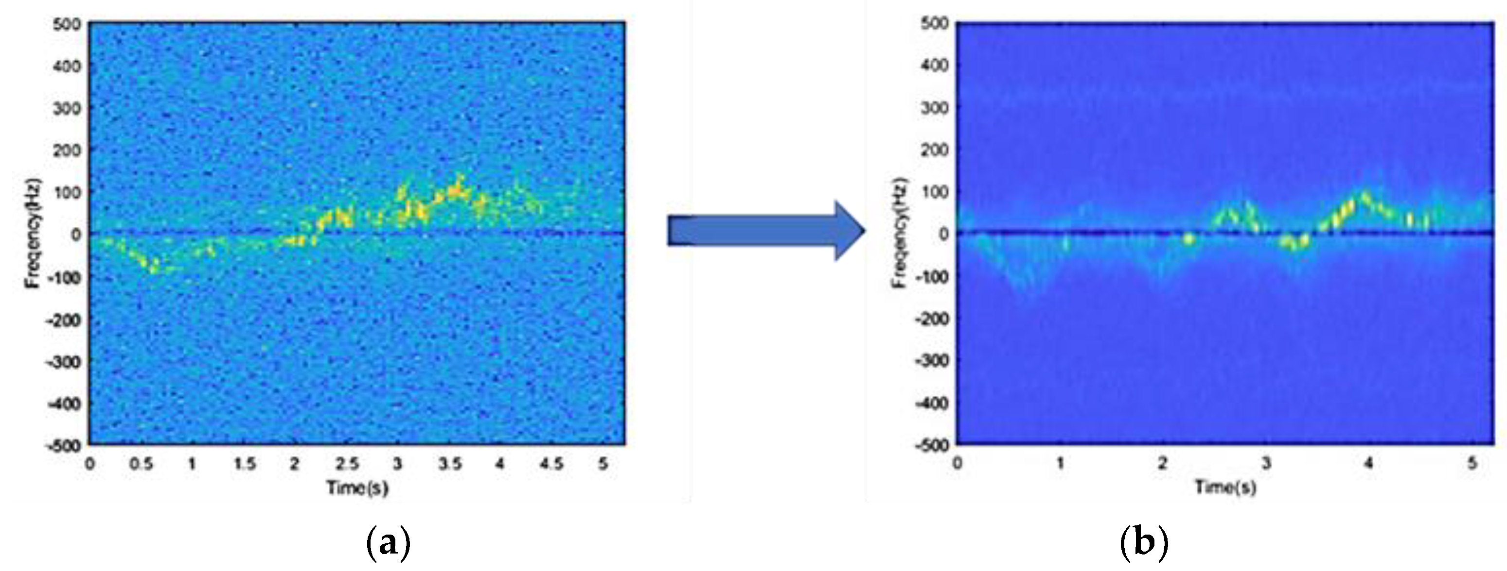
- (3)
- Noise reduction
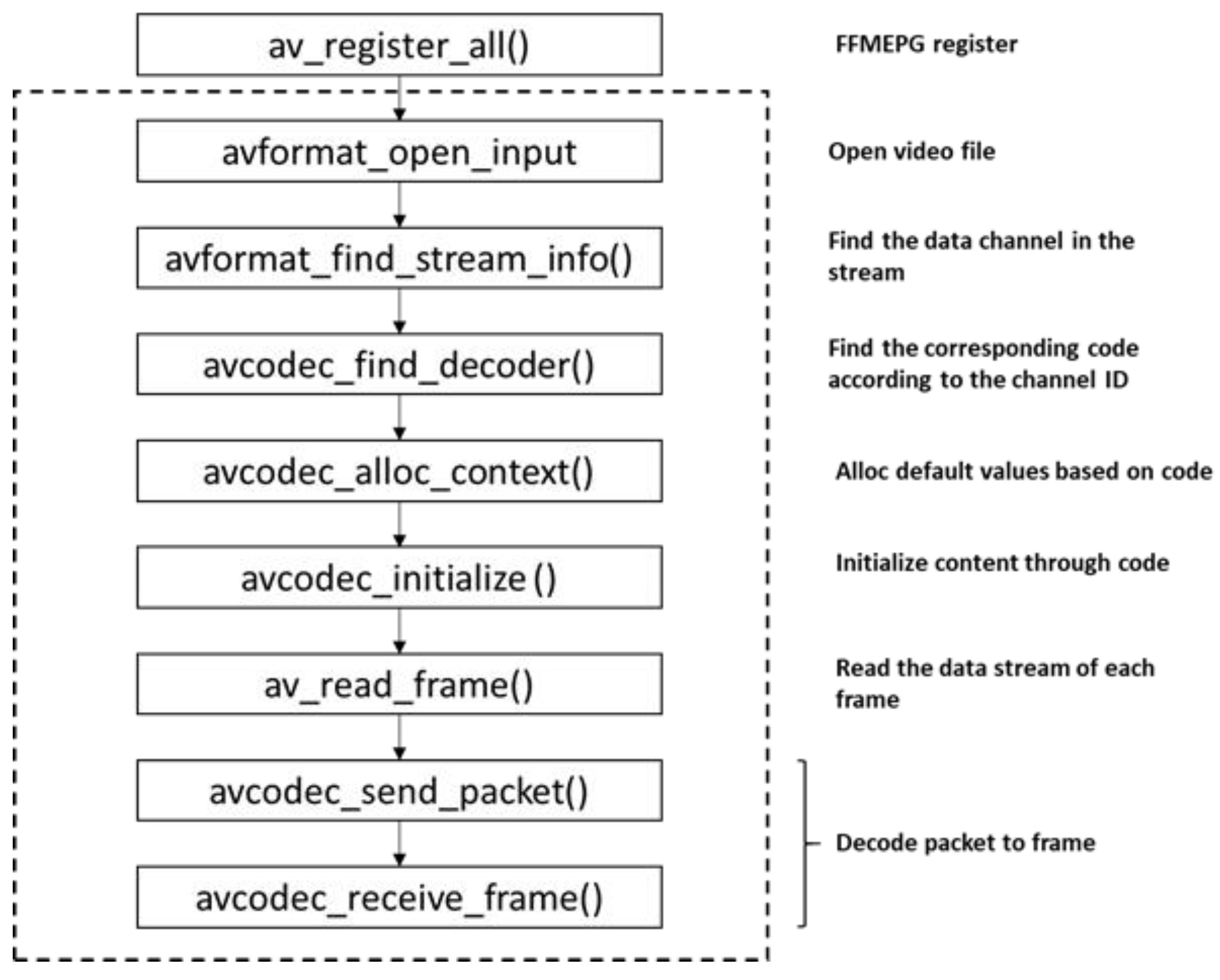
3.3.2. Video Data
3.4. Model Design
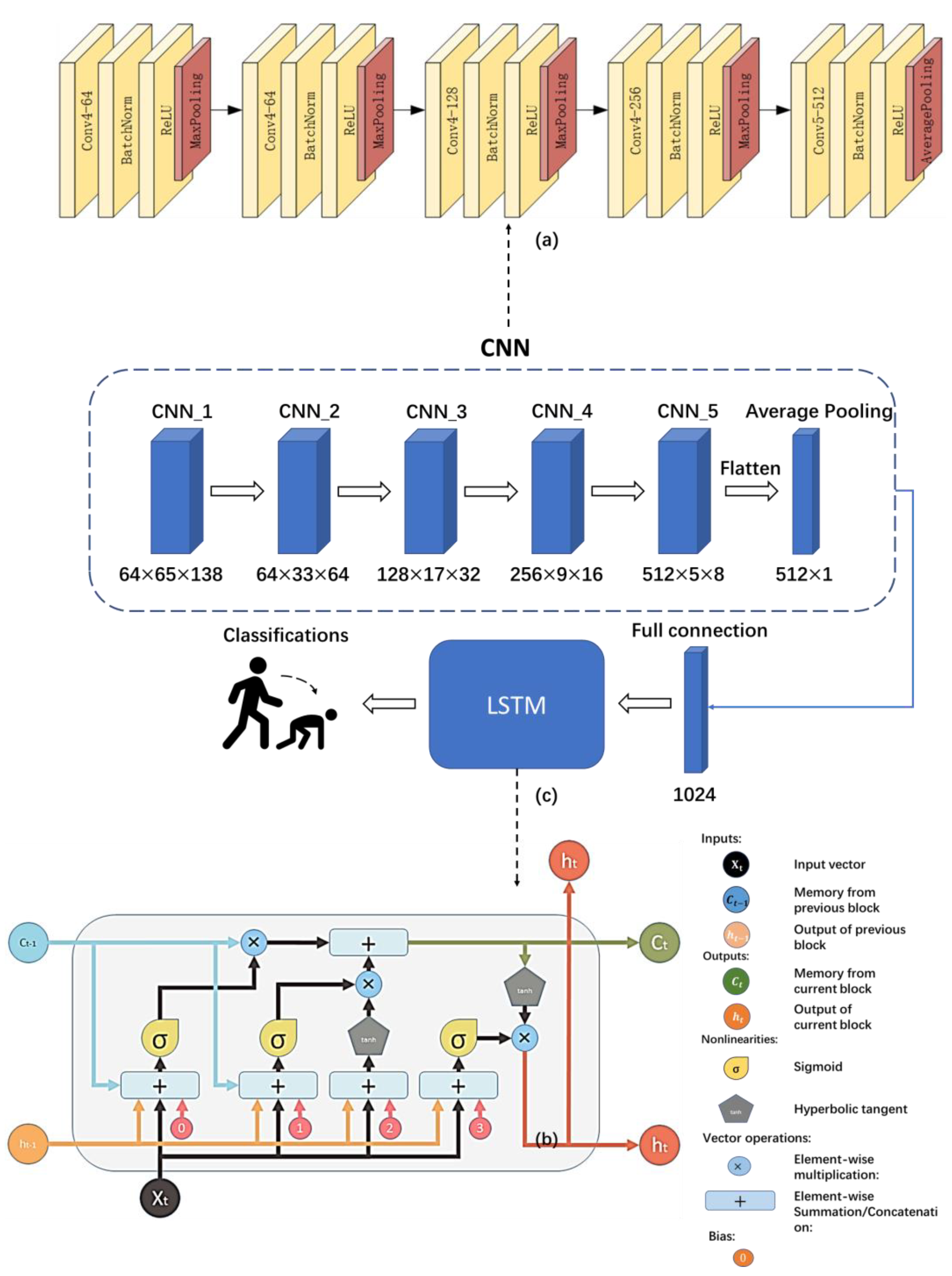
3.4.1. Combined CNN-LSTM Network
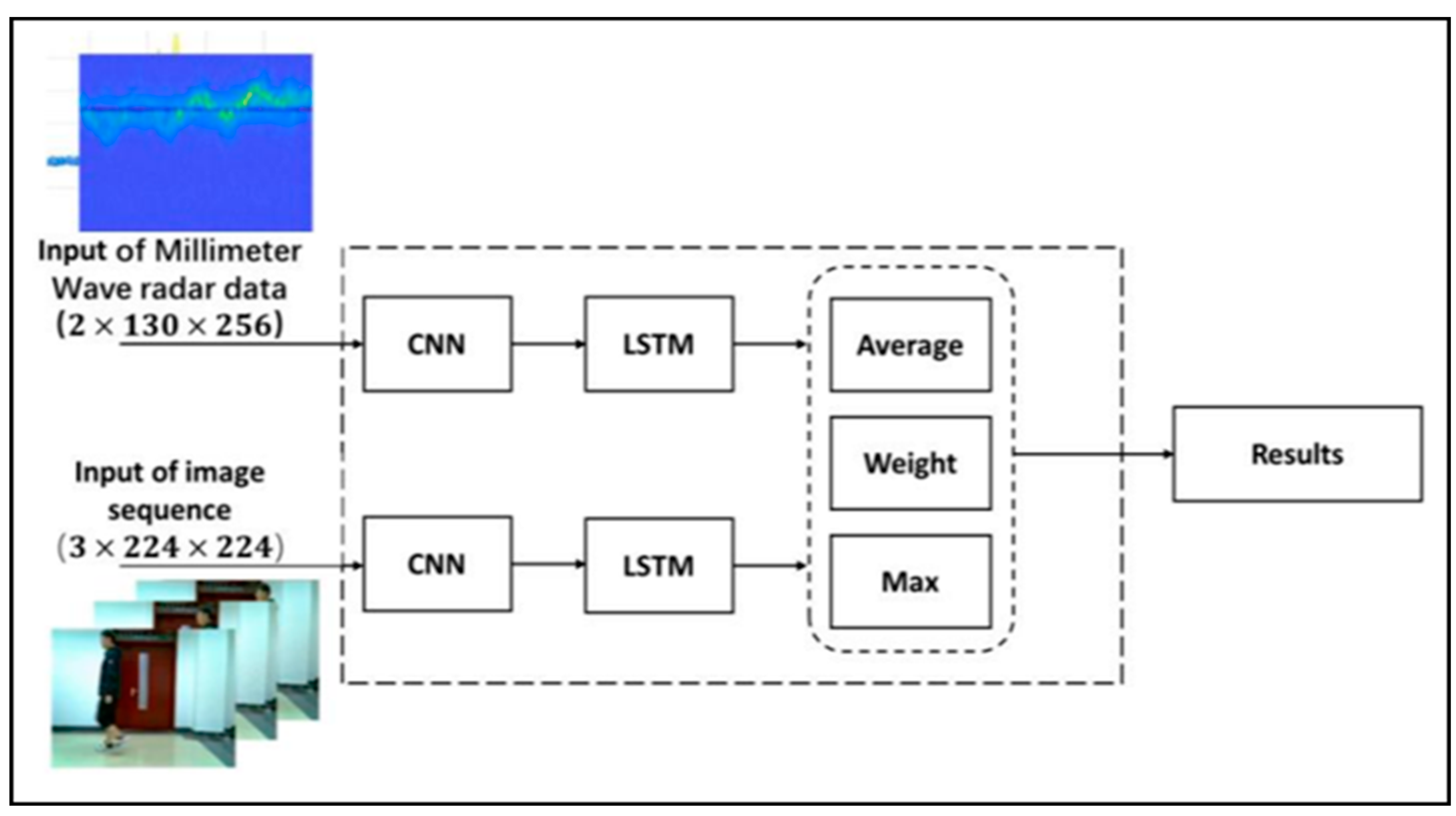
3.4.2. Multi-Sensor Data Fusion Algorithms
- (1)
- Data level fusion
- (2)
- Feature level fusion
- (a)
- Feature addition
- (b)
- Feature concatenation
- (3)
- Decision level Fusion algorithm
- (a)
- Decision level average fusion (DLAF)
- (b)
- Decision-level weights fusion (DLWF)
- (c)
- Decision level maximum fusion (DLMF)
4. System Test
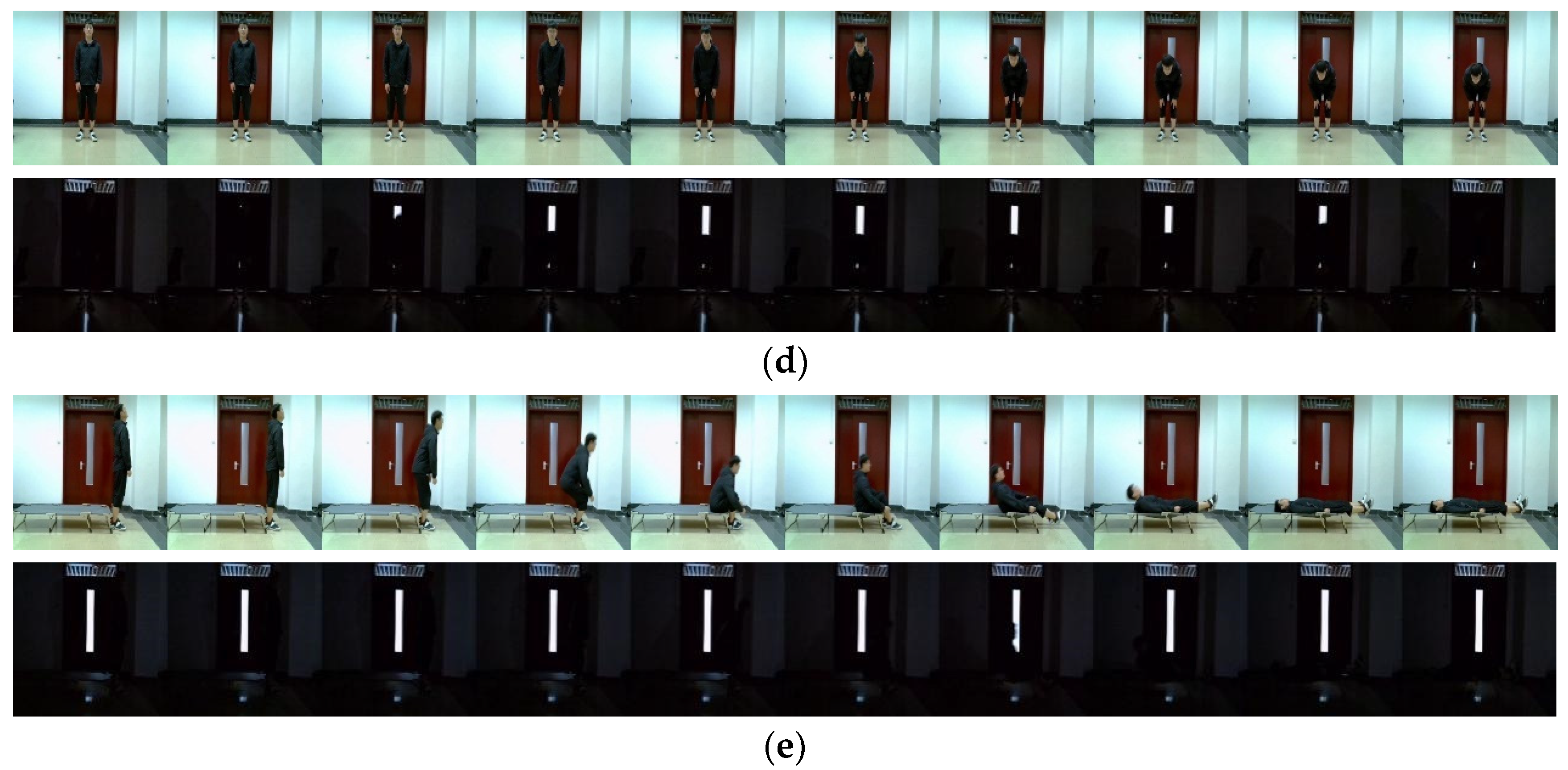
4.1. Experimental Data Collection
4.2. Evaluation Metrics
- (1)
- Accuracy
- (2)
- Confusion Matrix
4.3. Experimental Results
4.3.1. Model Comparison
4.3.2. Algorithm Comparison
5. Summary
Author Contributions
Funding
Institutional Review Board Statement
Informed Consent Statement
Data Availability Statement
Conflicts of Interest
References
- De Miguel, K.; Brunete, A.; Hernando, M.; Gambao, E. Home Camera-Based Fall Detection System for the Elderly. Sensors 2017, 17, 2864. [Google Scholar] [CrossRef]
- Zhao, Y.; Zhou, H.; Lu, S.; Liu, Y.; An, X.; Liu, Q. Human Activity Recognition Based on Non-Contact Radar Data and Improved PCA Method. Appl. Sci. 2022, 12, 7124. [Google Scholar] [CrossRef]
- Alonso, M.; Brunete, A.; Hernando, M.; Gambao, E. Background-Subtraction Algorithm Optimization for Home Camera-Based Night-Vision Fall Detectors. IEEE Access 2019, 7, 152399–152411. [Google Scholar] [CrossRef]
- Fan, K.; Wang, P.; Zhuang, S. Human fall detection using slow feature analysis. Multimed. Tools Appl. 2018, 78, 9101–9128. [Google Scholar] [CrossRef]
- Núñez-Marcos, A.; Azkune, G.; Arganda-Carreras, I. Vision-Based Fall Detection with Convolutional Neural Networks. Wirel. Commun. Mob. Comput. 2017, 2017, 9474806. [Google Scholar] [CrossRef]
- Feichtenhofer, C.; Pinz, A.; Zisserman, A. Convolutional Two-Stream Network Fusion for Video Action Recognition. In Proceedings of the 2016 IEEE Conference on Computer Vision and Pattern Recognition (CVPR), Las Vegas, NV, USA, 27–30 June 2016. [Google Scholar]
- Kondo, K.; Hasegawa, T. Sensor-Based Human Activity Recognition Using Adaptive Class Hierarchy. Sensors 2021, 21, 7743. [Google Scholar] [CrossRef] [PubMed]
- Kang, J.; Shin, J.; Shin, J.; Lee, D.; Choi, A. Robust Human Activity Recognition by Integrating Image and Accelerometer Sensor Data Using Deep Fusion Network. Sensors 2021, 22, 174. [Google Scholar] [CrossRef] [PubMed]
- Xu, T.; Zhou, Y. Elders’ fall detection based on biomechanical features using depth camera. Int. J. Wavelets Multiresolution Inf. Process. 2018, 16, 1840005. [Google Scholar] [CrossRef]
- Zhang, D.; Gao, H.; Dai, H.; Shi, X. Two-stream Graph Attention Convolutional for Video Action Recognition. In Proceedings of the 2021 IEEE 15th International Conference on Big Data Science and Engineering (BigDataSE), Shenyang, China, 20–22 October 2021. [Google Scholar]
- Khraief, C.; Benzarti, F.; Amiri, H. Elderly fall detection based on multi-stream deep convolutional networks. Multimed. Tools Appl. 2020, 79, 19537–19560. [Google Scholar] [CrossRef]
- Nandagopal, S.; Karthy, G.; Oliver, A.S.; Subha, M. Optimal Deep Convolutional Neural Network with Pose Estimation for Human Activity Recognition. Comput. Syst. Sci. Eng. 2022, 44, 1719–1733. [Google Scholar] [CrossRef]
- Wong, W.K.; Lim, H.L.; Loo, C.K.; Lim, W.S. Home Alone Faint Detection Surveillance System Using Thermal Camera. In Proceedings of the 2010 Second International Conference on Computer Research and Development, Kuala Lumpur, Malaysia, 7–10 May 2010. [Google Scholar]
- Batchuluun, G.; Nguyen, D.T.; Pham, T.D.; Park, C.; Park, K.R. Action recognition from thermal videos. IEEE Access. 2019, 7, 103893–103917. [Google Scholar] [CrossRef]
- Yong, C.Y.; Sudirman, R.; Chew, K.M. Dark Environment Motion Analysis Using Scalable Model and Vector Angle Technique. Appl. Mech. Mater. 2014, 654, 310–314. [Google Scholar] [CrossRef]
- Ulhaq, A. Action Recognition in the Dark via Deep Representation Learning. In Proceedings of the 2018 IEEE International Conference on Image Processing, Applications and Systems (IPAS), Sophia Antipolis, France, 12–14 December 2018; pp. 131–136. [Google Scholar] [CrossRef]
- Igual, R.; Medrano, C.; Plaza, I. Challenges, issues and trends in fall detection systems. Biomed. Eng. Online 2013, 12, 66. [Google Scholar] [CrossRef] [PubMed]
- Liu, L.; Popescu, M.; Skubic, M.; Rantz, M. An Automatic Fall Detection Framework Using Data Fusion of Doppler Radar and Motion Sensor Network. In Proceedings of the 36th Annual International Conference of the IEEE-Engineering-in-Medicine-and-Biology-Society (EMBC), Chicago, IL, USA, 26–30 August 2014. [Google Scholar]
- Jokanovic, B.; Amin, M.; Ahmad, F. Radar fall motion detection using deep learning. In Proceedings of the 2016 IEEE Radar Conference (RadarConf), Philadelphia, PA, USA, 2–6 May 2016. [Google Scholar] [CrossRef]
- Erol, B.; Amin, M.G.; Boashash, B. Range-Doppler radar sensor fusion for fall detection. In Proceedings of the 2017 IEEE Radar Conference (RadarConf), Seattle, WA, USA, 8–12 May 2017. [Google Scholar] [CrossRef]
- Sadreazami, H.; Bolic, M.; Rajan, S. Fall Detection Using Standoff Radar-Based Sensing and Deep Convolutional Neural Network. IEEE Trans. Circuits Syst. II Express Briefs 2019, 67, 197–201. [Google Scholar] [CrossRef]
- Tsuchiyama, K.; Kajiwara, A. Accident detection and health-monitoring UWB sensor in toilet. In Proceedings of the IEEE Topical Conference on Wireless Sensors and Sensor Networks (WiSNet), Orlando, FL, USA, 20–23 January 2019. [Google Scholar]
- Bhattacharya, A.; Vaughan, R. Deep Learning Radar Design for Breathing and Fall Detection. IEEE Sensors J. 2020, 20, 5072–5085. [Google Scholar] [CrossRef]
- Wang, C.; Lu, W.; Redmond, S.J.; Stevens, M.C.; Lord, S.R.; Lovell, N.H. A Low-Power Fall Detector Balancing Sensitivity and False Alarm Rate. IEEE J. Biomed. Health Inform. 2017, 22, 1929–1937. [Google Scholar] [CrossRef] [PubMed]
- Cornacchia, M.; Ozcan, K.; Zheng, Y.; Velipasalar, S. A Survey on Activity Detection and Classification Using Wearable Sensors. IEEE Sensors J. 2016, 17, 386–403. [Google Scholar] [CrossRef]
- Shoaib, M.; Bosch, S.; Incel, O.D.; Scholten, H.; Havinga, P.J.M. Complex Human Activity Recognition Using Smartphone and Wrist-Worn Motion Sensors. Sensors 2016, 16, 426. [Google Scholar] [CrossRef] [PubMed]
- Brezmes, T.; Gorricho, J.-L.; Cotrina, J. Activity Recognition from Accelerometer Data on a Mobile Phone. In Proceedings of the 10th International Work-Conference on Artificial Neural Networks (IWANN 2009), Salamanca, Spain, 10–12 June 2009. [Google Scholar]
- Capela, N.A.; Lemaire, E.D.; Baddour, N. Feature Selection for Wearable Smartphone-Based Human Activity Recognition with Able bodied, Elderly, and Stroke Patients. PLoS ONE 2015, 10, e0124414. [Google Scholar] [CrossRef] [PubMed]
- Kuncheva, L.I. Combining Pattern Classifiers: Methods and Algorithms; John Wiley & Sons: Hoboken, NJ, USA, 2004. [Google Scholar]
- Min, J.-K.; Cho, S.-B. Activity recognition based on wearable sensors using selection/fusion hybrid ensemble. In Proceedings of the 2011 IEEE International Conference on Systems, Man, and Cybernetics, Anchorage, AK, USA, 9–12 October 2011; pp. 1319–1324. [Google Scholar] [CrossRef]
- Lecun, Y.; Fu, J.H.; Bottou, L. Learning methods for generic object recognition with invariance to pose and lighting. In Proceedings of the 2004 IEEE Computer Society Conference on Computer Vision and Pattern Recognition, Washington, DC, USA, 27 June–2 July 2004. [Google Scholar]
- Zhang, Z. A Flexible New Technique for Camera Calibration. IEEE Trans. Pattern Anal. Mach. Intell. 2000, 22, 1330–1334. [Google Scholar] [CrossRef]


| Number | Name | Parameter |
|---|---|---|
| 1 | Sensor | CMOS |
| 2 | Pixel | 3 million |
| 3 | Capture Size | 1280 × 720 |
| 4 | Resolution | 1280 × 720 |
| 5 | Max FPS | 30 frames/s |
| 6 | Interface | USB 2.0 |
| Name | Introduction |
|---|---|
| Antenna | AN7105 dual-polarized patch antenna |
| RF front-end chip | AWR1843, supports frequency ranges from 60 GHz to 64 GHz |
| Digital signal processor chip | Uses high-performance floating-point DSP architecture |
| Microcontroller | RM57L843, uses ARM Cortex-R5F architecture |
| Number | Name | Parameter |
|---|---|---|
| 1 | Types | FMCW |
| 2 | Tuning Frequency | 60–64 GHz |
| 3 | Number of Receivers | 4 |
| 4 | Number of Transmitter | 3 |
| 5 | Azimuth FOV (deg) | |
| 6 | Azimuth Angular Resolution (deg) | 15 |
| 7 | Elevation FOV (deg) | |
| 8 | Elevation Angular Resolution (deg) | 58 |
| 9 | Arm CPU | ARM R4F @ 200 MHz |
| 10 | Memory (kb) | 1792 |
| Specification | Performance Parameters |
|---|---|
| Operating frequency | 76 GHz to 81 GHz |
| Receiver sensitivity | −80 dBm |
| Ranging range | maximum 8 m |
| Field of view (FOV) | 60 degrees (horizontal) × 20 degrees (vertical) |
| Data output | Distance, speed, angle, target information, etc. |
| Environment | Proportion | Activity | (Quantity, Proportion) |
|---|---|---|---|
| Normal light | Train set (1200, 40%) Test set (300, 10%) | Sitting | (300, 10%) |
| Squatting | (300, 10%) | ||
| Walking | (300, 10%) | ||
| Bending | (300, 10%) | ||
| Falling | (300, 10%) | ||
| Low-light | Train set (1200, 40%) Test set (300, 10%) | Sitting | (300, 10%) |
| Squatting | (300, 10%) | ||
| Walking | (300, 10%) | ||
| Bending | (300, 10%) | ||
| Falling | (300, 10%) |
| Sensor | Input Data | Environment | Model | Activities | ||||
|---|---|---|---|---|---|---|---|---|
| Sitting | Bending | Walking | Squatting | Falling | ||||
| Radar | Spectrogram | Low-light | CNN | 78.94% | 89.74% | 97.37% | 77.50% | 78.94% |
| RNN | 33.92% | 73.62% | 17.21% | 12.58% | 31.56% | |||
| CNN-LSTM | 95.83% | 89.29% | 100.00% | 78.12% | 80.00% | |||
| Camera | Image sequence | Normal light | CNN | 94.48% | 91.36% | 98.87% | 85.62% | 98.23% |
| RNN | 92.58% | 94.27% | 98.91% | 80.23% | 93.41% | |||
| CNN-LSTM | 98.26% | 97.87% | 100.00% | 96.12% | 98.24% | |||
| Image sequence | Low-light | CNN | 58.64% | 39.59% | 58.62% | 36.87% | 40.12% | |
| RNN | 70.53% | 43.51% | 52.09% | 77.50% | 62.91% | |||
| CNN-LSTM | 63.17% | 57.36% | 53.37% | 12.58% | 69.23% | |||
| Predict | Bending | Falling | Sitting | Squatting | Walking | |
|---|---|---|---|---|---|---|
| True | ||||||
| Bending | 57 | 21 | 11 | 4 | 6 | |
| Falling | 10 | 57 | 12 | 6 | 2 | |
| Sitting | 9 | 13 | 63 | 2 | 4 | |
| Squatting | 9 | 13 | 21 | 49 | 5 | |
| Walking | 11 | 9 | 14 | 13 | 54 | |
| Predict | Bending | Falling | Sitting | Squatting | Walking | |
|---|---|---|---|---|---|---|
| True | ||||||
| Bending | 89 | 0 | 4 | 7 | 0 | |
| Falling | 0 | 80 | 4 | 8 | 8 | |
| Sitting | 0 | 0 | 96 | 4 | 0 | |
| Squatting | 3 | 3 | 16 | 78 | 0 | |
| Walking | 0 | 0 | 0 | 0 | 100 | |
| Algorithm | Activities | |||||
|---|---|---|---|---|---|---|
| Sitting | Bending | Walking | Squatting | Falling | ||
| Data level fusion | 94.55% | 94.12% | 98.04% | 95.92% | 95.91% | |
| Feature level fusion | Addition | 86.96% | 89.11% | 90.53% | 84.76% | 93.52% |
| Concatenation | 83.04% | 92.38% | 86.96% | 85.29% | 90.27% | |
| Decision level fusion | DLAF | 91.26% | 99.12% | 98.96% | 92.11% | 96.94% |
| DLWF | 89.29% | 95.24% | 91.30% | 86.27% | 91.15% | |
| DLMF | 93.20% | 97.35% | 97.92% | 93.86% | 98.98% | |
| Predict | Bending | Falling | Sitting | Squatting | Walking | |
|---|---|---|---|---|---|---|
| True | ||||||
| Bending | 94 | 2 | 4 | 0 | 0 | |
| Falling | 0 | 96 | 4 | 0 | 0 | |
| Sitting | 0 | 4 | 95 | 2 | 0 | |
| Squatting | 0 | 2 | 2 | 96 | 0 | |
| Walking | 0 | 0 | 0 | 2 | 98 | |
| Predict | Bending | Falling | Sitting | Squatting | Walking | |
|---|---|---|---|---|---|---|
| True | ||||||
| Bending | 89/92 | 5/4 | 4/4 | 4/0 | 0/0 | |
| Falling | 1/5 | 94/90 | 1/2 | 5/2 | 0/1 | |
| Sitting | 1/2 | 2/1 | 87/83 | 10/12 | 0/13 | |
| Squatting | 0/0 | 1/2 | 1/12 | 85/85 | 3/1 | |
| Walking | 1/2 | 2/2 | 3/5 | 3/3 | 91/87 | |
| Predict | Bending | Falling | Sitting | Squatting | Walking | |
|---|---|---|---|---|---|---|
| True | ||||||
| Bending | 99/97/95 | 0/0/3 | 1/2/1 | 0/1/1 | 0/0/0 | |
| Falling | 2/0/5 | 97/99/91 | 0/0/3 | 1/0/0 | 0/1/1 | |
| Sitting | 1/1/1 | 0/0/0 | 91/93/89 | 6/5/7 | 2/1/3 | |
| Squatting | 0/0/0 | 1/0/0 | 1/6/11 | 92/94/86 | 0/0/3 | |
| Walking | 0/0/2 | 0/1/1 | 0/1/5 | 1/0/0 | 99/98/86 | |
Disclaimer/Publisher’s Note: The statements, opinions and data contained in all publications are solely those of the individual author(s) and contributor(s) and not of MDPI and/or the editor(s). MDPI and/or the editor(s) disclaim responsibility for any injury to people or property resulting from any ideas, methods, instructions or products referred to in the content. |
© 2023 by the authors. Licensee MDPI, Basel, Switzerland. This article is an open access article distributed under the terms and conditions of the Creative Commons Attribution (CC BY) license (https://creativecommons.org/licenses/by/4.0/).
Share and Cite
Zhou, H.; Zhao, Y.; Liu, Y.; Lu, S.; An, X.; Liu, Q. Multi-Sensor Data Fusion and CNN-LSTM Model for Human Activity Recognition System. Sensors 2023, 23, 4750. https://doi.org/10.3390/s23104750
Zhou H, Zhao Y, Liu Y, Lu S, An X, Liu Q. Multi-Sensor Data Fusion and CNN-LSTM Model for Human Activity Recognition System. Sensors. 2023; 23(10):4750. https://doi.org/10.3390/s23104750
Chicago/Turabian StyleZhou, Haiyang, Yixin Zhao, Yanzhong Liu, Sichao Lu, Xiang An, and Qiang Liu. 2023. "Multi-Sensor Data Fusion and CNN-LSTM Model for Human Activity Recognition System" Sensors 23, no. 10: 4750. https://doi.org/10.3390/s23104750