
A Novel Approach for Brain Tumor Classification Using an Ensemble of Deep and Hand-Crafted Features

Abstract
:1. Introduction
- We present a novel method based on an ensemble of deep and hand-crafted features to classify brain tumors in MR images.
- Per our knowledge, this is the first-ever study based on a feature-level ensemble of VGG16 and GLCM features to classify brain tumors.
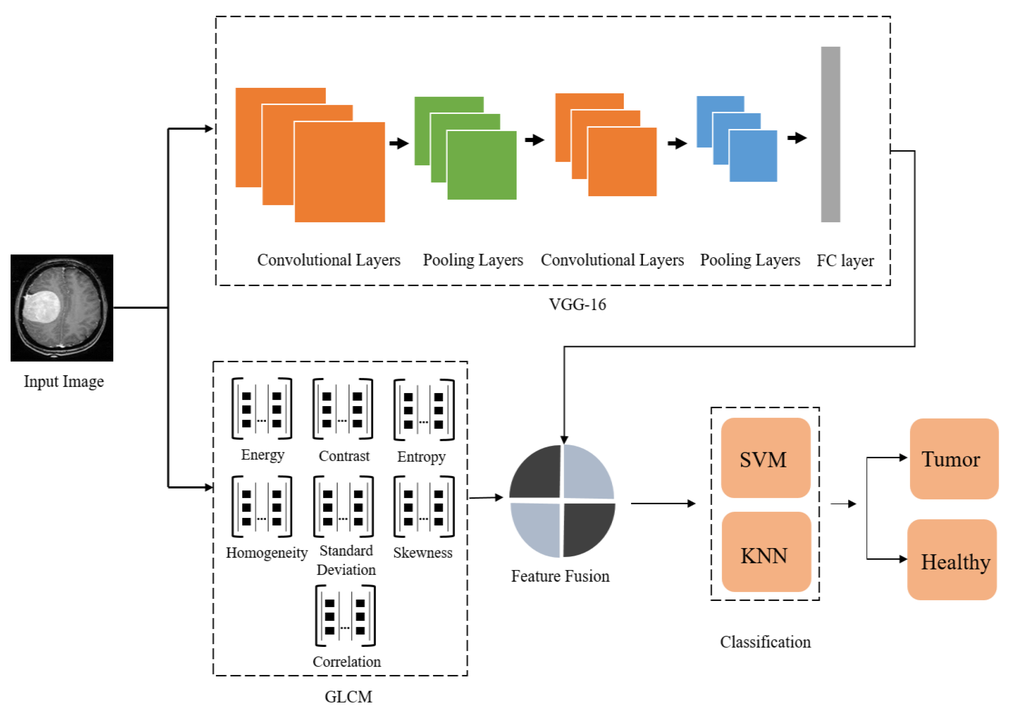
- Our framework consists of three main core steps: deep feature extraction via CNN, that is, through the VGG16 model, hand-crafted feature computation via GLCM, creating an ensemble vector of these FVs, and finally, classification using SVM and KNN.
- The proposed method effectively classifies brain tumors because the fusion of the GLCM and deep FV computes an effective set of image features, resulting in better discrimination of tumor and normal images.
- The results indicate the efficacy of the presented approach as compared to existing methodologies.
2. Related Work
- Compute the Euclidean or Mahalanobis distance between the target and sampled plots.
- Arrange samples according to the calculated distances.
- Select the optimal k-nearest neighbors heuristically based on the RMSE obtained by the cross-validation technique.
- Compute a weighted average of the inverse distance to the k multivariate nearest neighbors.
3. Proposed Methodology
3.1. Feature Extraction
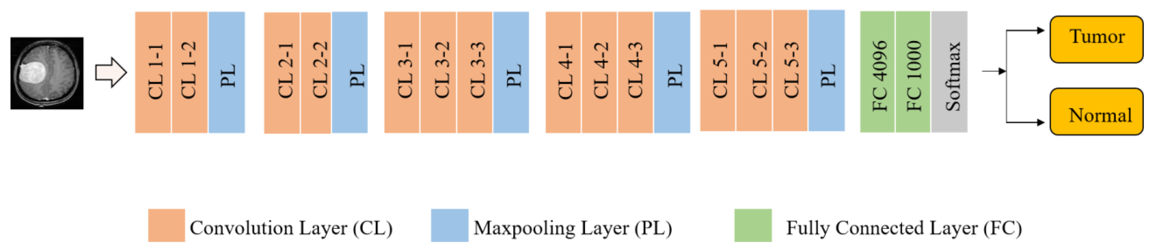
3.1.1. Deep Feature Extraction Using VGG-16
3.1.2. Hand-Crafted Feature Extraction Using GLCM
3.2. Feature Ensemble
3.3. Classification
4. Results
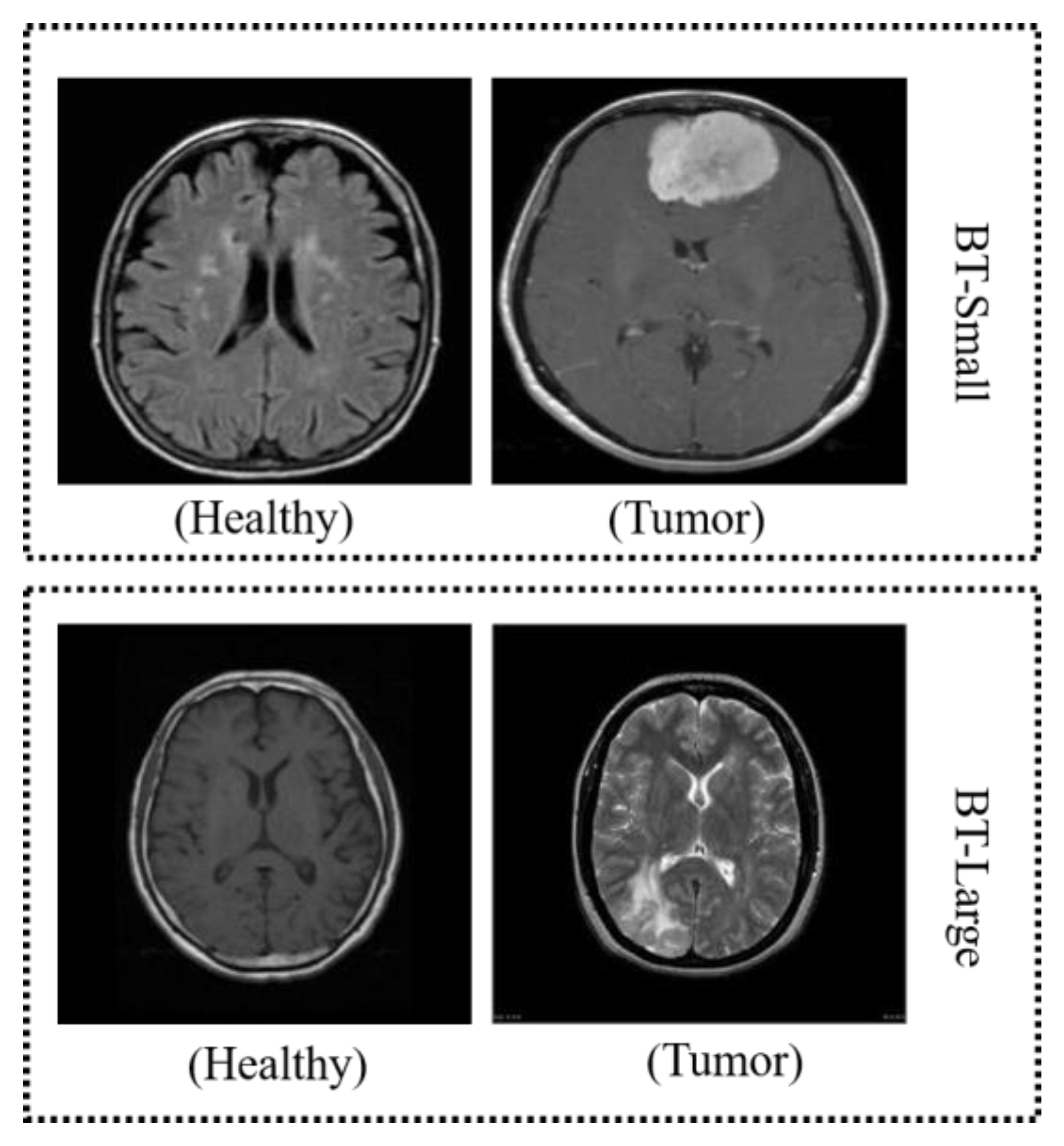
4.1. Dataset
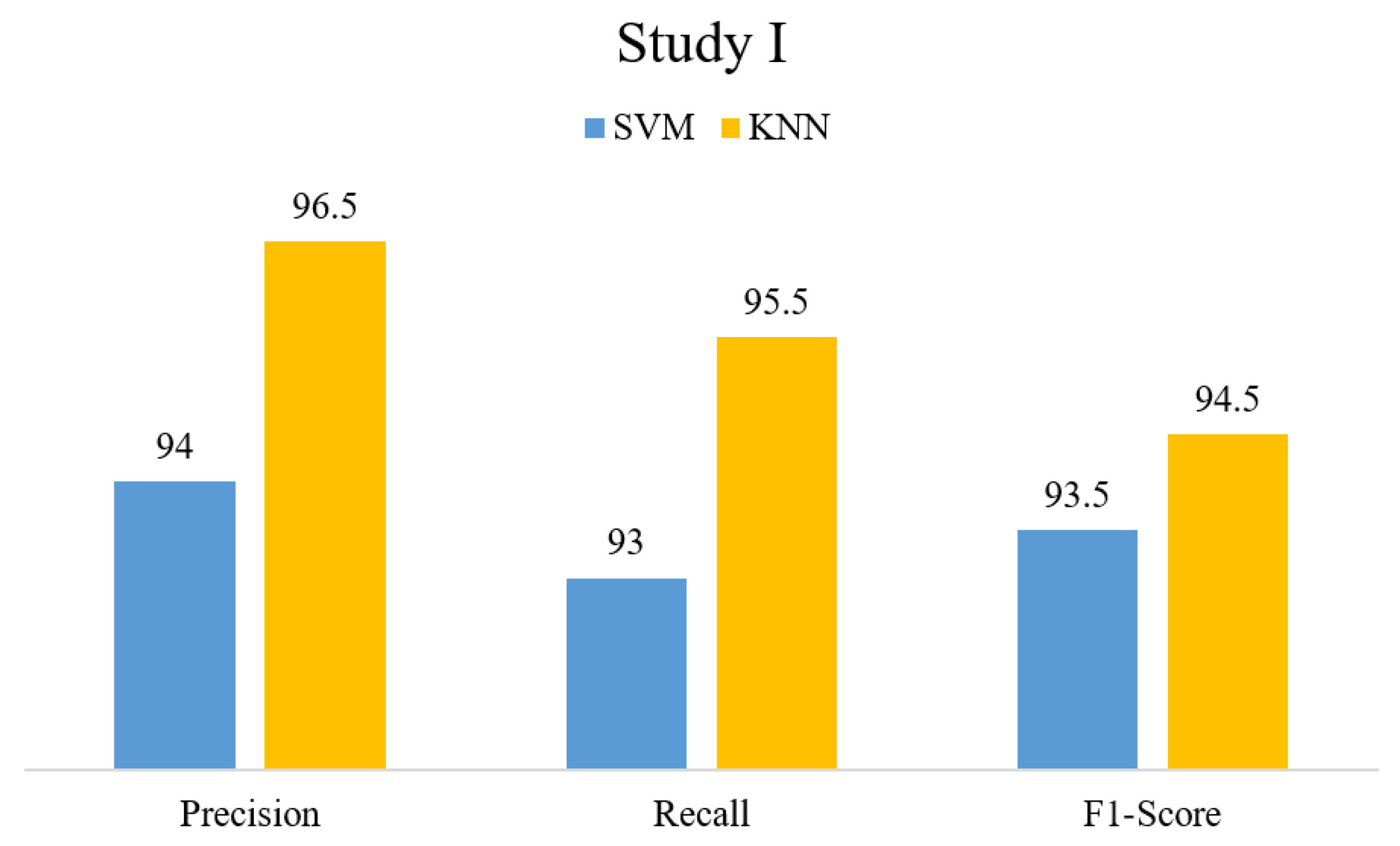
4.2. Evaluation Parameters
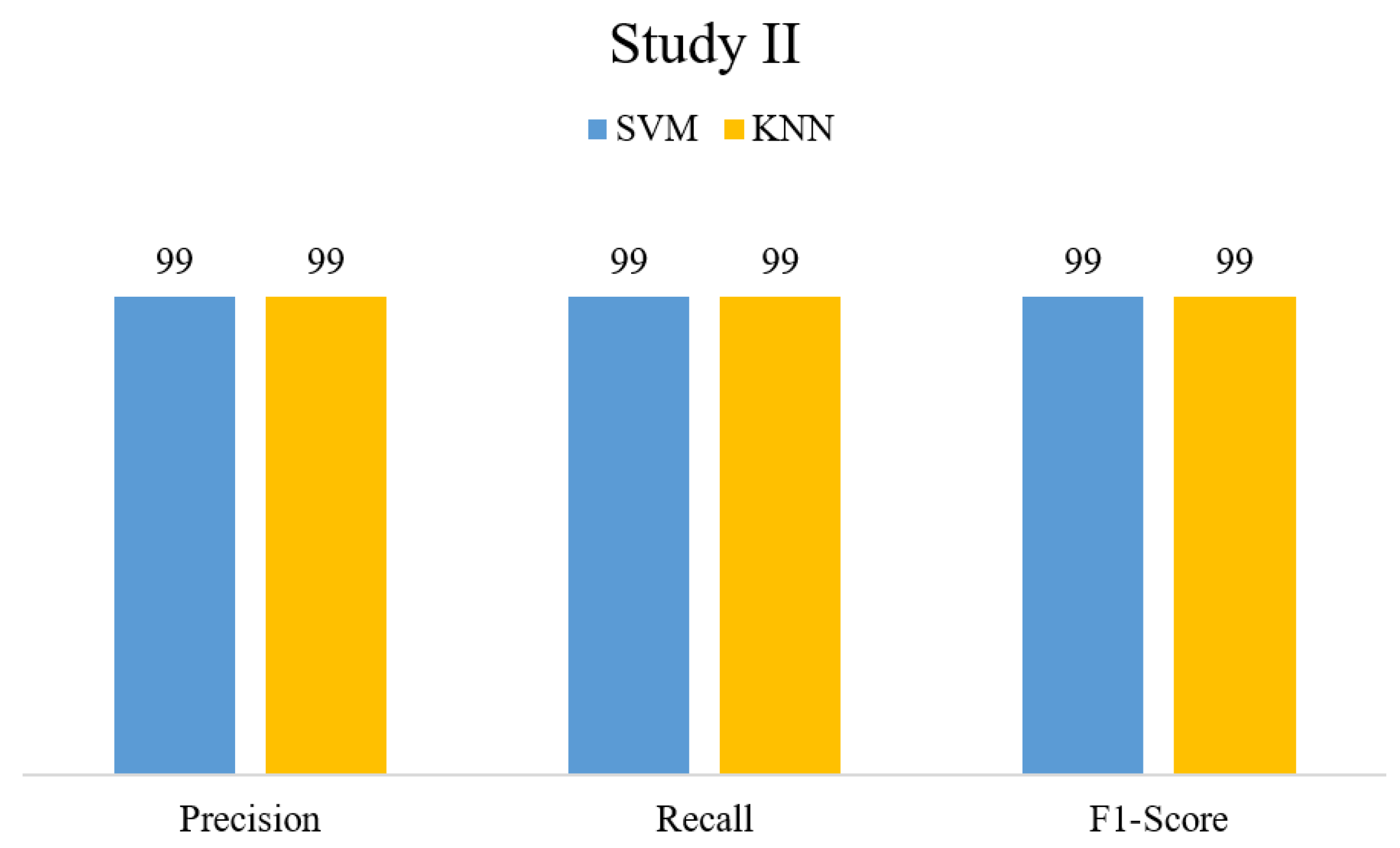
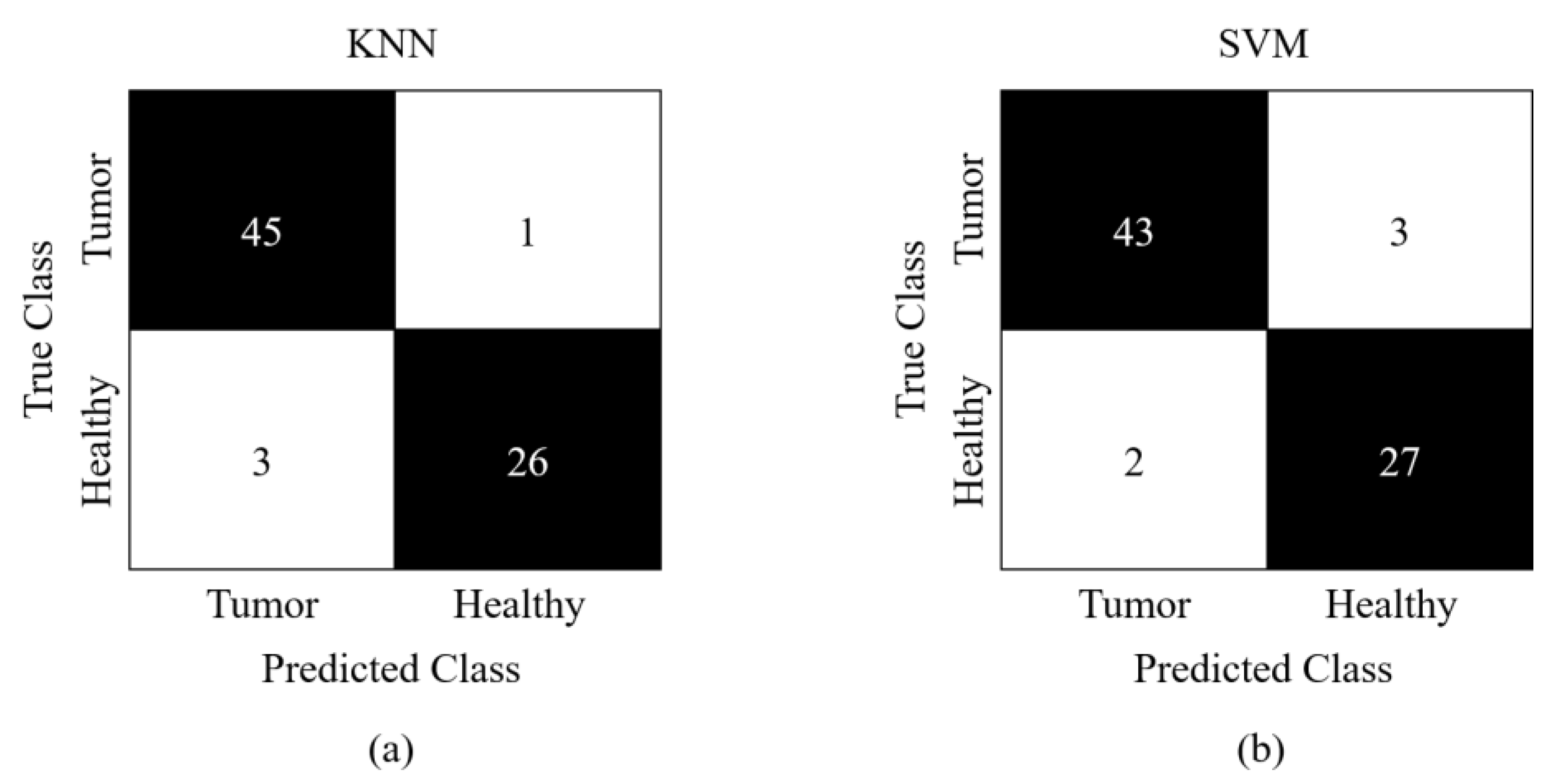
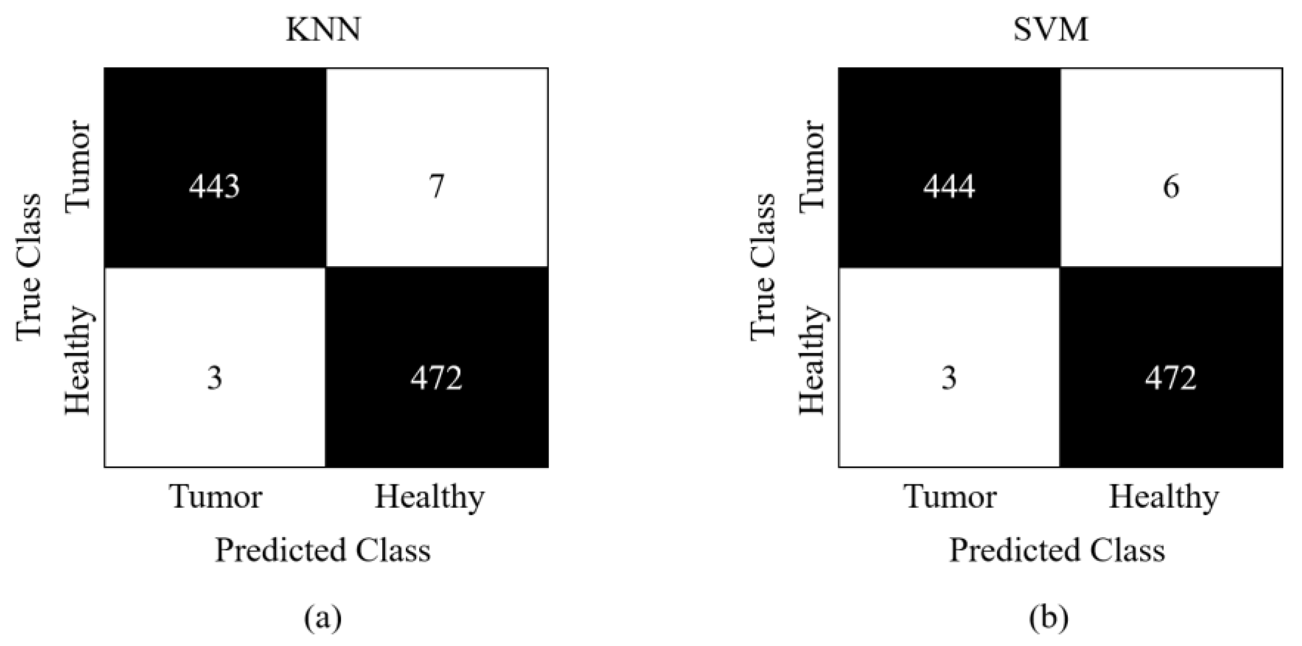
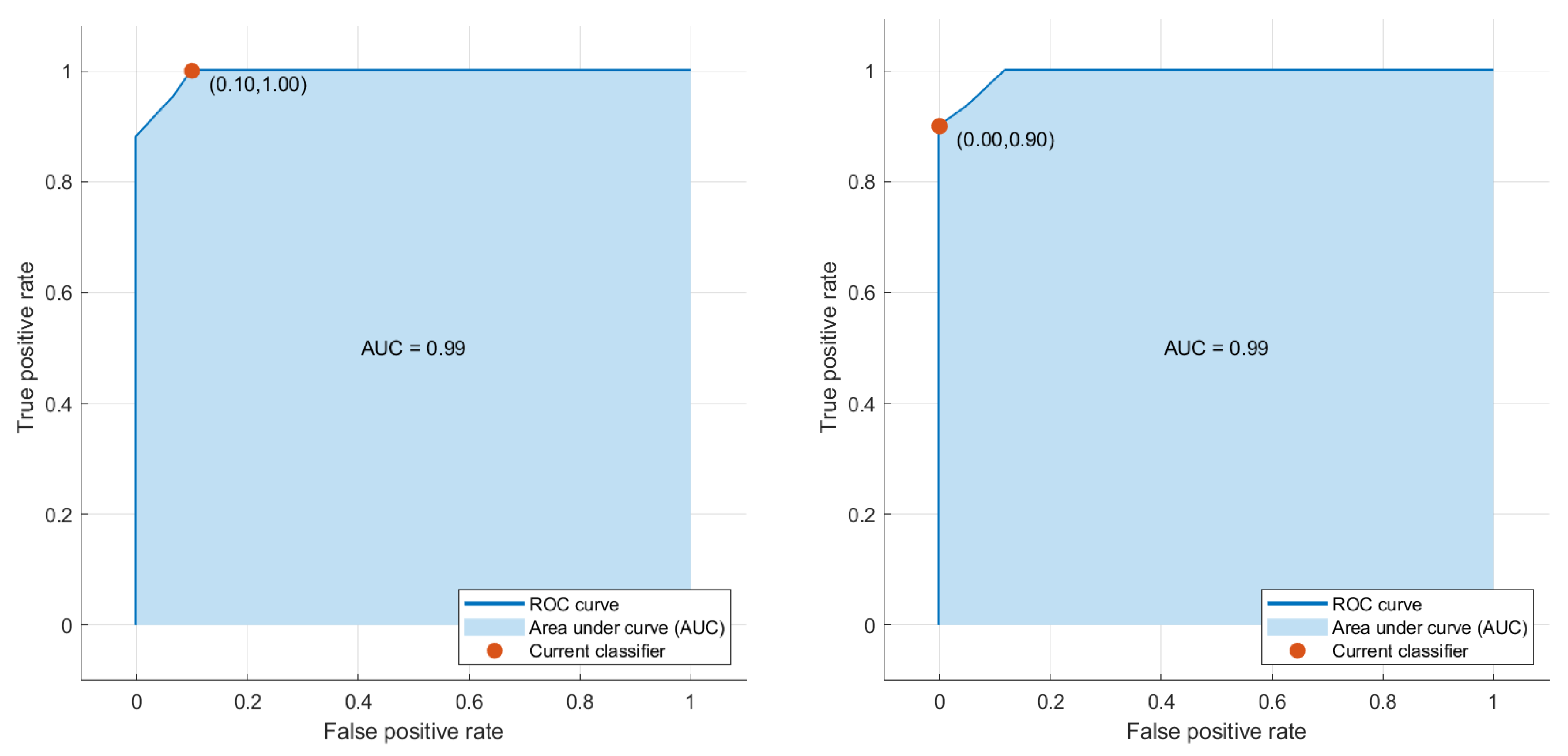
4.3. Results Obtained from the Proposed Framework
4.4. Cross-Dataset Validation
4.5. Comparison with Existing Approaches
5. Conclusions
Author Contributions
Funding
Informed Consent Statement
Data Availability Statement
Conflicts of Interest
References
- Anitha, R.; Raja, D.S.S. Development of computer-aided approach for brain tumor detection using random forest classifier. Int. J. Imaging Syst. Technol. 2017, 28, 48–53. [Google Scholar] [CrossRef]
- Lu, J.; Nguyen, M.; Yan, W.Q. Deep learning methods for human behavior recognition. In Proceedings of the 2020 35th International Conference on Image and Vision Computing New Zealand (IVCNZ), Wellington, New Zealand, 25–27 November 2020; pp. 1–6. [Google Scholar]
- Al-Okaili, R.N.; Krejza, J.; Wang, S.; Woo, J.H.; Melhem, E.R. Advanced MR Imaging Techniques in the Diagnosis of Intraaxial Brain Tumors in Adults. Radiographics 2006, 26, S173–S189. [Google Scholar] [CrossRef] [PubMed]
- Badža, M.M.; Barjaktarović, M. Segmentation of Brain Tumors from MRI Images Using Convolutional Autoencoder. Appl. Sci. 2021, 11, 4317. [Google Scholar] [CrossRef]
- Nisar, D.-E.; Amin, R.; Shah, N.-U.; Al Ghamdi, M.A.; Almotiri, S.H.; Alruily, M. Healthcare Techniques Through Deep Learning: Issues, Challenges and Opportunities. IEEE Access 2021, 9, 98523–98541. [Google Scholar] [CrossRef]
- Swati, Z.N.K.; Zhao, Q.; Kabir, M.; Ali, F.; Ali, Z.; Ahmed, S.; Lu, J. Brain tumor classification for MR images using transfer learning and fine-tuning. Comput. Med. Imaging Graph. 2019, 75, 34–46. [Google Scholar] [CrossRef]
- Anaraki, A.K.; Ayati, M.; Kazemi, F. Magnetic resonance imaging-based brain tumor grades classification and grading via convolutional neural networks and genetic algorithms. Biocybern. Biomed. Eng. 2018, 39, 63–74. [Google Scholar] [CrossRef]
- Habib, H.; Amin, R.; Ahmed, B.; Hannan, A. Hybrid algorithms for brain tumor segmentation, classification and feature extraction. J. Ambient. Intell. Humaniz. Comput. 2022, 13, 1–22. [Google Scholar]
- Hussain, S.; Anwar, S.M.; Majid, M. Segmentation of glioma tumors in brain using deep convolutional neural network. Neurocomputing 2018, 282, 248–261. [Google Scholar] [CrossRef]
- Muhammad, K.; Khan, S.; Del Ser, J.; de Albuquerque, V.H.C. Deep Learning for Multigrade Brain Tumor Classification in Smart Healthcare Systems: A Prospective Survey. IEEE Trans. Neural Netw. Learn. Syst. 2020, 32, 507–522. [Google Scholar] [CrossRef]
- Mzoughi, H.; Njeh, I.; Wali, A.; Ben Slima, M.; BenHamida, A.; Mhiri, C.; Ben Mahfoudhe, K. Deep Multi-Scale 3D Convolutional Neural Network (CNN) for MRI Gliomas Brain Tumor Classification. J. Digit. Imaging 2020, 33, 903–915. [Google Scholar] [CrossRef]
- Sejuti, Z.A.; Islam, M.S. An Efficient Method to Classify Brain Tumor using CNN and SVM. In Proceedings of the IEEE 2nd International Conference on Robotics, Electrical and Signal Processing Techniques (ICREST), Dhaka, Bangladesh, 5–7 January 2021; pp. 644–648. [Google Scholar]
- Abiwinanda, N.; Hanif, M.; Hesaputra, S.T.; Handayani, A.; Mengko, T.R. Brain tumor classification using convolutional neural network. In Proceedings of the World Congress on Medical Physics and Biomedical Engineering 2018, Prague, Czech Republic, 3–5 May 2019; pp. 183–189. [Google Scholar]
- Khan, A.H.; Abbas, S.; Khan, M.A.; Farooq, U.; Khan, W.A.; Siddiqui, S.Y.; Ahmad, A. Intelligent Model for Brain Tumor Identification Using Deep Learning. Appl. Comput. Intell. Soft Comput. 2022, 2022, 1–10. [Google Scholar] [CrossRef]
- Alanazi, M.F.; Ali, M.U.; Hussain, S.J.; Zafar, A.; Mohatram, M.; Irfan, M.; AlRuwaili, R.; Alruwaili, M.; Ali, N.H.; Albarrak, A.M. Brain Tumor/Mass Classification Framework Using Magnetic-Resonance-Imaging-Based Isolated and Developed Transfer Deep-Learning Model. Sensors 2022, 22, 372. [Google Scholar] [CrossRef] [PubMed]
- Afshar, P.; Plataniotis, K.N.; Mohammadi, A. Capsule Networks for Brain Tumor Classification Based on MRI Images and Coarse Tumor Boundaries. In Proceedings of the ICASSP 2019—2019 IEEE International Conference on Acoustics, Speech and Signal Processing (ICASSP), Brighton, UK, 12–17 May 2019; pp. 1368–1372. [Google Scholar]
- Noreen, N.; Palaniappan, S.; Qayyum, A.; Ahmad, I.; Alassafi, M.O. Brain Tumor Classification Based on Fine-Tuned Models and the Ensemble Method. Comput. Mater. Contin. 2021, 67, 3967–3982. [Google Scholar] [CrossRef]
- Kang, J.; Ullah, Z.; Gwak, J. MRI-Based Brain Tumor Classification Using Ensemble of Deep Features and Machine Learning Classifiers. Sensors 2021, 21, 2222. [Google Scholar] [CrossRef]
- Waghmare, V.K.; Kolekar, M.H. Brain Tumor Classification Using Deep Learning. In Internet of Things for Healthcare Technologies; Springer: Berlin/Heidelberg, Germany, 2020; pp. 155–175. [Google Scholar]
- Naser, M.A.; Deen, M.J. Brain tumor segmentation and grading of lower-grade glioma using deep learning in MRI images. Comput. Biol. Med. 2020, 121, 103758. [Google Scholar] [CrossRef]
- Masood, M.; Nazir, T.; Nawaz, M.; Mehmood, A.; Rashid, J.; Kwon, H.-Y.; Mahmood, T.; Hussain, A. A Novel Deep Learning Method for Recognition and Classification of Brain Tumors from MRI Images. Diagnostics 2021, 11, 744. [Google Scholar] [CrossRef]
- Sajjad, M.; Khan, S.; Muhammad, K.; Wu, W.; Ullah, A.; Baik, S.W. Multi-grade brain tumor classification using deep CNN with extensive data augmentation. J. Comput. Sci. 2018, 30, 174–182. [Google Scholar] [CrossRef]
- Amin, J.; Sharif, M.; Yasmin, M.; Fernandes, S.L. A distinctive approach in brain tumor detection and classification using MRI. Pattern Recognit. Lett. 2017, 139, 118–127. [Google Scholar] [CrossRef]
- Kaplan, K.; Kaya, Y.; Kuncan, M.; Ertunç, H.M. Brain tumor classification using modified local binary patterns (LBP) feature extraction methods. Med. Hypotheses 2020, 139, 109696. [Google Scholar] [CrossRef]
- Bahadure, N.B.; Ray, A.K.; Thethi, H.P. Image Analysis for MRI Based Brain Tumor Detection and Feature Extraction Using Biologically Inspired BWT and SVM. Int. J. Biomed. Imaging 2017, 2017, 1–12. [Google Scholar] [CrossRef]
- Garg, G.; Garg, R. Brain Tumor Detection and Classification based on Hybrid Ensemble Classifier. arXiv 2021, arXiv:2101.00216. [Google Scholar]
- Minz, A.; Mahobiya, C. MR image classification using adaboost for brain tumor type. In Proceedings of the 2017 IEEE 7th International Advance Computing Conference (IACC), Hyderabad, India, 5–7 January 2017; pp. 701–705. [Google Scholar]
- Raja, P.S.J.B.; Engineering, B. Brain tumor classification using a hybrid deep autoencoder with Bayesian fuzzy clustering-based segmentation approach. Biocybern. Biomed. Eng. 2020, 40, 440–453. [Google Scholar] [CrossRef]
- Ali, F.; Khan, S.; Abbas, A.W.; Shah, B.; Hussain, T.; Song, D.; Ei-Sappagh, S.; Singh, J. A Two-Tier Framework Based on GoogLeNet and YOLOv3 Models for Tumor Detection in MRI. Comput. Mater. Contin. 2022, 72, 73–92. [Google Scholar] [CrossRef]
- Das, S.; Nayak, G.; Saba, L.; Kalra, M.; Suri, J.S.; Saxena, S. An artificial intelligence framework and its bias for brain tumor segmentation: A narrative review. Comput. Biol. Med. 2022, 143, 105273. [Google Scholar] [CrossRef]
- Khan, M.A.; Ashraf, I.; Alhaisoni, M.; Damaševičius, R.; Scherer, R.; Rehman, A.; Bukhari, S.A.C. Multimodal Brain Tumor Classification Using Deep Learning and Robust Feature Selection: A Machine Learning Application for Radiologists. Diagnostics 2020, 10, 565. [Google Scholar] [CrossRef]
- Irsheidat, S.; Duwairi, R. Brain tumor detection using artificial convolutional neural networks. In Proceedings of the 2020 11th International Conference on Information and Communication Systems (ICICS), Irbid, Jordan, 7–9 April 2020; pp. 197–203. [Google Scholar]
- Kesav, N.; Jibukumar, M. Efficient and low complex architecture for detection and classification of Brain Tumor using RCNN with Two Channel CNN. J. King Saud Univ.-Comput. Inf. Sci. 2021, 34, 6229–6242. [Google Scholar] [CrossRef]
- Shahajad, M.; Gambhir, D.; Gandhi, R. Features extraction for classification of brain tumor MRI images using support vector machine. In Proceedings of the 2021 11th International Conference on Cloud Computing, Data Science & Engineering (Confluence), Noida, India, 28–29 January 2021; pp. 767–772. [Google Scholar] [CrossRef]
- Mathswork. Feature Extraction for Machine Learning and Deep Learning. Available online: https://www.mathworks.com/discovery/feature-extraction.html (accessed on 17 August 2022).
- Fu, P.; Chu, L.; Hou, Z.; Xing, J.; Gao, J.; Guo, C. Deep learning based velocity prediction with consideration of road structure. In Proceedings of the 2021 5th CAA International Conference on Vehicular Control and Intelligence (CVCI), Tianjin, China, 29–31 October 2021; IEEE: Piscataway, NJ, USA, 2021; pp. 1–5. [Google Scholar]
- Buduma, N.; Buduma, N.; Papa, J. Fundamentals of Deep Learning; O’Reilly Media, Inc.: Sebastopol, CA, USA, 2022. [Google Scholar]
- Sedik, A.; Hammad, M.; El-Samie, F.E.A.; Gupta, B.B.; El-Latif, A.A.A. Efficient deep learning approach for augmented detection of Coronavirus disease. Neural Comput. Appl. 2021, 34, 11423–11440. [Google Scholar] [CrossRef] [PubMed]
- Simonyan, K.; Zisserman, A. Very deep convolutional networks for large-scale image recognition. arXiv 2014, arXiv:1409.1556. [Google Scholar]
- Nadeem, M.W.; Ghamdi, M.A.A.; Hussain, M.; Khan, M.A.; Khan, K.M.; Almotiri, S.H.; Butt, S.A. Brain tumor analysis empowered with deep learning: A review, taxonomy, and future challenges. Brain Sci. 2020, 10, 118. [Google Scholar] [CrossRef]
- Kumar, S.; Fred, A.L.; Padmanabhan, P.; Gulyas, B.; Kumar, H.A.; Miriam, L.J. Deep Learning Algorithms in Medical Image Processing for Cancer Diagnosis: Overview, Challenges and Future. Deep. Learn. Cancer Diagn. 2021, 37–66. [Google Scholar]
- O’Shea, K.; Nash, R. An introduction to convolutional neural networks. arXiv 2015, arXiv:1511.08458. [Google Scholar]
- Nanni, L.; Ghidoni, S.; Brahnam, S. Handcrafted vs. non-handcrafted features for computer vision classification. Pattern Recognit. 2017, 71, 158–172. [Google Scholar] [CrossRef]
- Haralick, R.M.; Shanmugam, K.; Dinstein, I.H. Textural Features for Image Classification. IEEE Trans. Syst. Man Cybern. 1973, 3, 610–621. [Google Scholar] [CrossRef]
- Humeau-Heurtier, A. Texture Feature Extraction Methods: A Survey. IEEE Access 2019, 7, 8975–9000. [Google Scholar] [CrossRef]
- Suthaharan, S. Support vector machine. In Machine Learning Models and Algorithms for Big Data Classification; Springer: Berlin/Heidelberg, Germany, 2016; pp. 207–235. [Google Scholar]
- Kibriya, H.; Amin, R.; Alshehri, A.H.; Masood, M.; Alshamrani, S.S.; Alshehri, A. A Novel and Effective Brain Tumor Classification Model Using Deep Feature Fusion and Famous Machine Learning Classifiers. Comput. Intell. Neurosci. 2022, 2022, 7897669. [Google Scholar] [CrossRef]
- Peterson, L.E. K-nearest neighbor. Scholarpedia 2009, 4, 1883. [Google Scholar] [CrossRef]
- Cai, J.; Li, J.; Li, W.; Wang, J. Deeplearning model used in text classification. In Proceedings of the 2018 15th International Computer Conference on Wavelet Active Media Technology and Information Processing (ICCWAMTIP), Chengdu, China, 14–16 December 2018; pp. 123–126. [Google Scholar]
- Semberecki, P.; Maciejewski, H. Deep learning methods for subject text classification of articles. In Proceedings of the 2017 Federated Conference on Computer Science and Information Systems (FedCSIS), Prague, Czech Republic, 3–6 September 2017; pp. 357–360. [Google Scholar]
- Zou, K.H.; O’Malley, A.J.; Mauri, L.J.C. Receiver-operating characteristic analysis for evaluating diagnostic tests and predictive models. Circulation 2007, 115, 654–657. [Google Scholar] [CrossRef]
- Hajian-Tilaki, K. Receiver operating characteristic (ROC) curve analysis for medical diagnostic test evaluation. Caspian J. Intern. Med. 2013, 4, 627. [Google Scholar]
- Ekelund, S. Roc Curves—What are they and how are they used? Point Care 2012, 11, 16–21. [Google Scholar] [CrossRef]
- Jiang, F.; Jiang, Y.; Zhi, H.; Dong, Y.; Li, H.; Ma, S.; Wang, Y.; Dong, Q.; Shen, H.; Wang, Y. Artificial intelligence in healthcare: Past, present and future. Stroke Vasc. Neurol. 2017, 2, 230–243. [Google Scholar] [CrossRef]
- Sultan, H.H.; Salem, N.M.; Al-Atabany, W. Multi-Classification of Brain Tumor Images Using Deep Neural Network. IEEE Access 2019, 7, 69215–69225. [Google Scholar] [CrossRef]
- Sharma, S.; Gupta, S.; Gupta, D.; Juneja, A.; Khatter, H.; Malik, S.; Bitsue, Z.K. Deep Learning Model for Automatic Classification and Prediction of Brain Tumor. J. Sens. 2022, 2022, 1–11. [Google Scholar] [CrossRef]
- Tazin, T.; Sarker, S.; Gupta, P.; Ibn Ayaz, F.; Islam, S.; Khan, M.M.; Bourouis, S.; Idris, S.A.; Alshazly, H. A Robust and Novel Approach for Brain Tumor Classification Using Convolutional Neural Network. Comput. Intell. Neurosci. 2021, 2021, 1–11. [Google Scholar] [CrossRef] [PubMed]


| Method | Dataset | Training Samples | Validation Samples |
|---|---|---|---|
| Study I | BT-small | 177 | 76 |
| Study II | BT-large | 2100 | 900 |
| FV | Study I Accuracy % | Study II Accuracy % | ||
|---|---|---|---|---|
| SVM | KNN | SVM | KNN | |
| VGG16 | 92.1 | 88.1 | 98.0 | 97.8 |
| GLCM | 72.0 | 84.0 | 96.1 | 96.0 |
| GLCM + VGG16 | 93.3 | 96.0 | 99.0 | 98.7 |
| Classifiers/ Method | Accuracy % | |
|---|---|---|
| Study I | Study II | |
| SVM | 92.0 | 99.6 |
| KNN | 90.0 | 99.2 |
Disclaimer/Publisher’s Note: The statements, opinions and data contained in all publications are solely those of the individual author(s) and contributor(s) and not of MDPI and/or the editor(s). MDPI and/or the editor(s) disclaim responsibility for any injury to people or property resulting from any ideas, methods, instructions or products referred to in the content. |
© 2023 by the authors. Licensee MDPI, Basel, Switzerland. This article is an open access article distributed under the terms and conditions of the Creative Commons Attribution (CC BY) license (https://creativecommons.org/licenses/by/4.0/).
Share and Cite
Kibriya, H.; Amin, R.; Kim, J.; Nawaz, M.; Gantassi, R. A Novel Approach for Brain Tumor Classification Using an Ensemble of Deep and Hand-Crafted Features. Sensors 2023, 23, 4693. https://doi.org/10.3390/s23104693
Kibriya H, Amin R, Kim J, Nawaz M, Gantassi R. A Novel Approach for Brain Tumor Classification Using an Ensemble of Deep and Hand-Crafted Features. Sensors. 2023; 23(10):4693. https://doi.org/10.3390/s23104693
Chicago/Turabian StyleKibriya, Hareem, Rashid Amin, Jinsul Kim, Marriam Nawaz, and Rahma Gantassi. 2023. "A Novel Approach for Brain Tumor Classification Using an Ensemble of Deep and Hand-Crafted Features" Sensors 23, no. 10: 4693. https://doi.org/10.3390/s23104693