
DSTEELNet: A Real-Time Parallel Dilated CNN with Atrous Spatial Pyramid Pooling for Detecting and Classifying Defects in Surface Steel Strips


Abstract
:1. Introduction
2. Related Work
3. Materials and Methods
3.1. Datasets
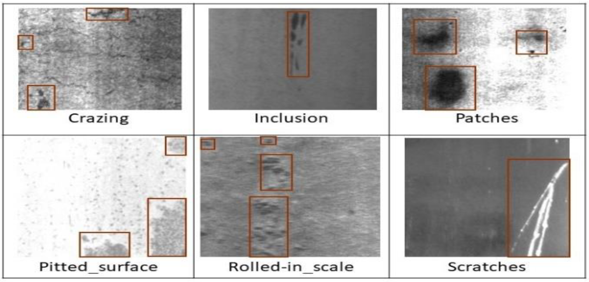
3.1.1. NEU Dataset Augmentation
GAN Architecture
Generating GNEU
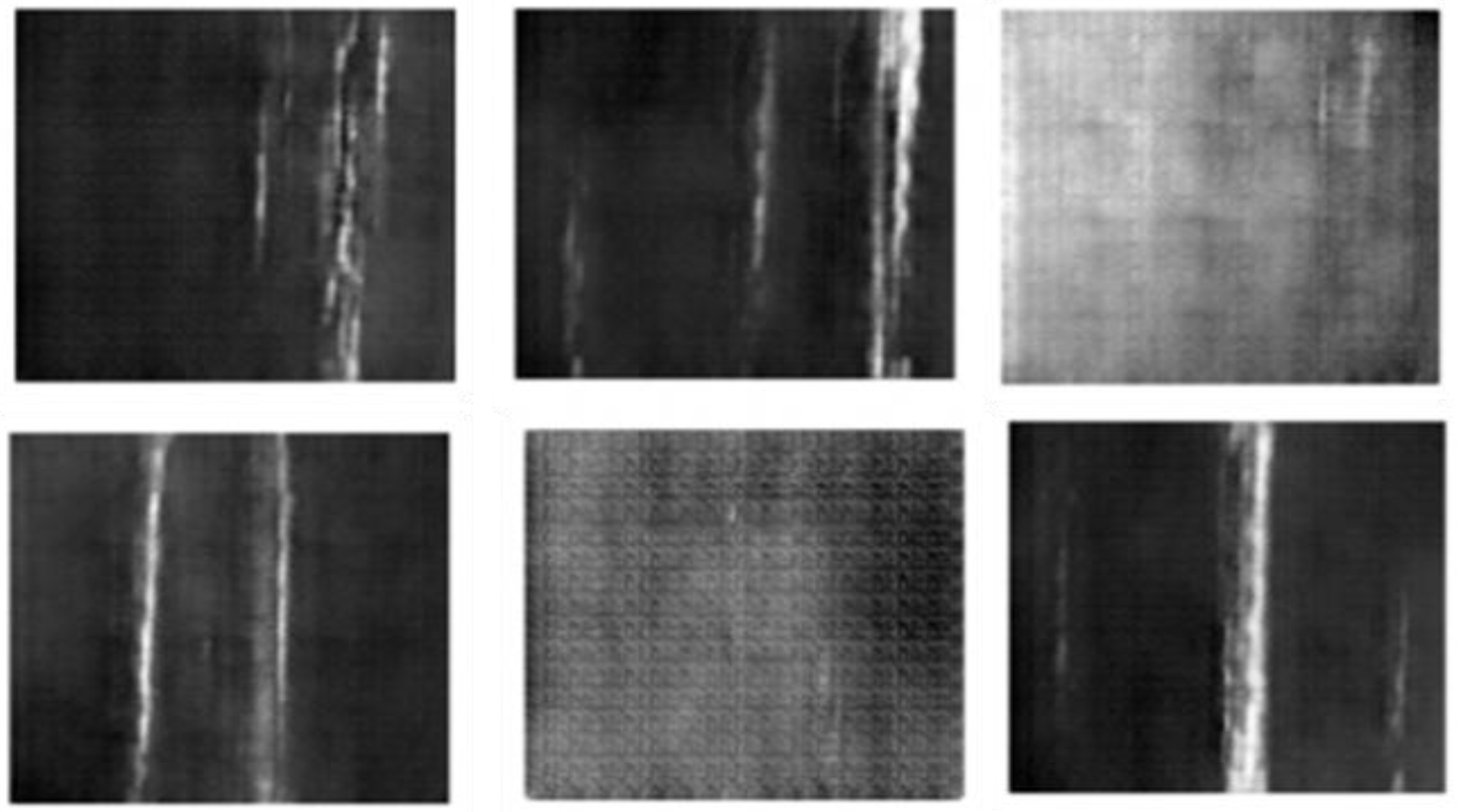
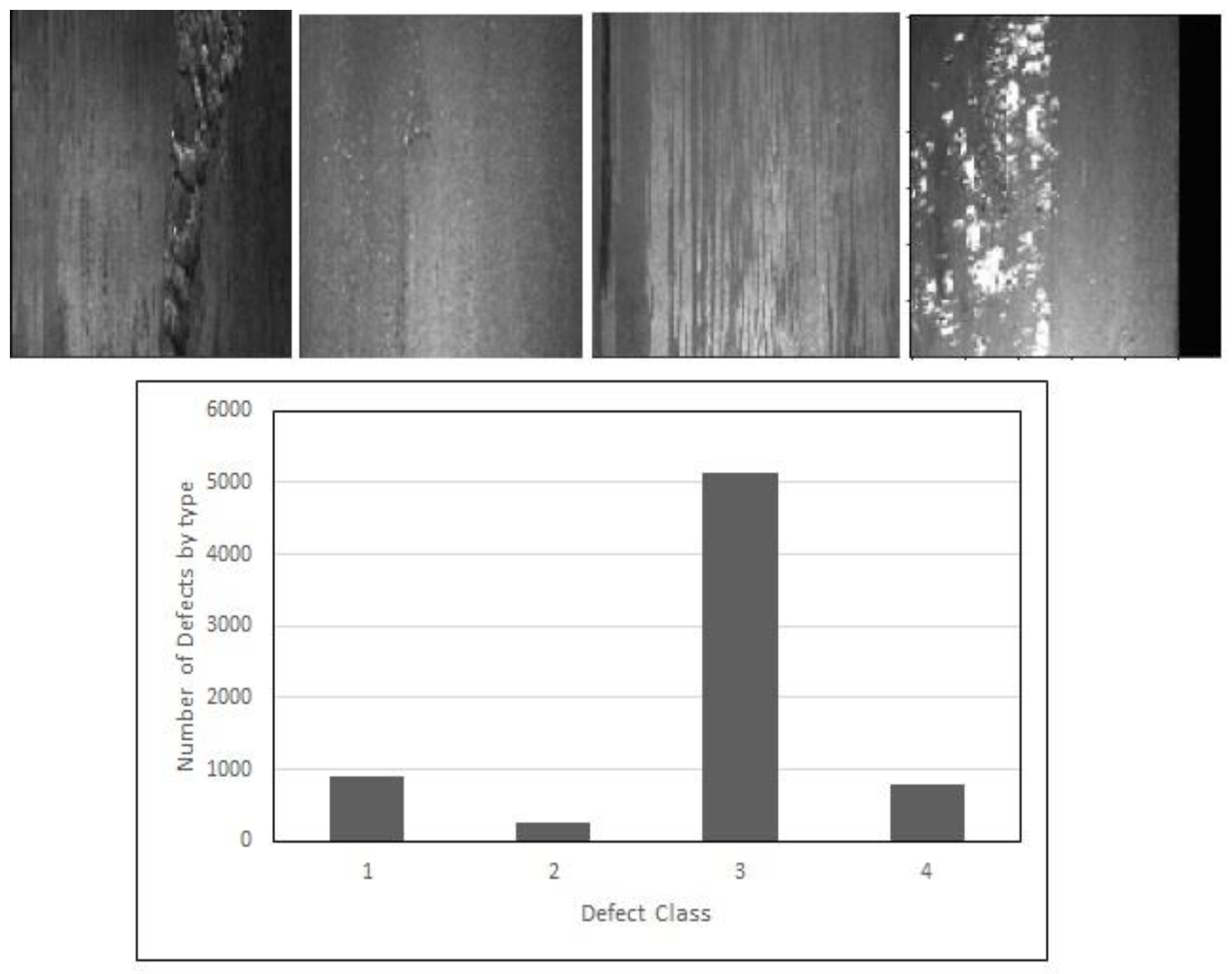
3.1.2. Severstal Dataset
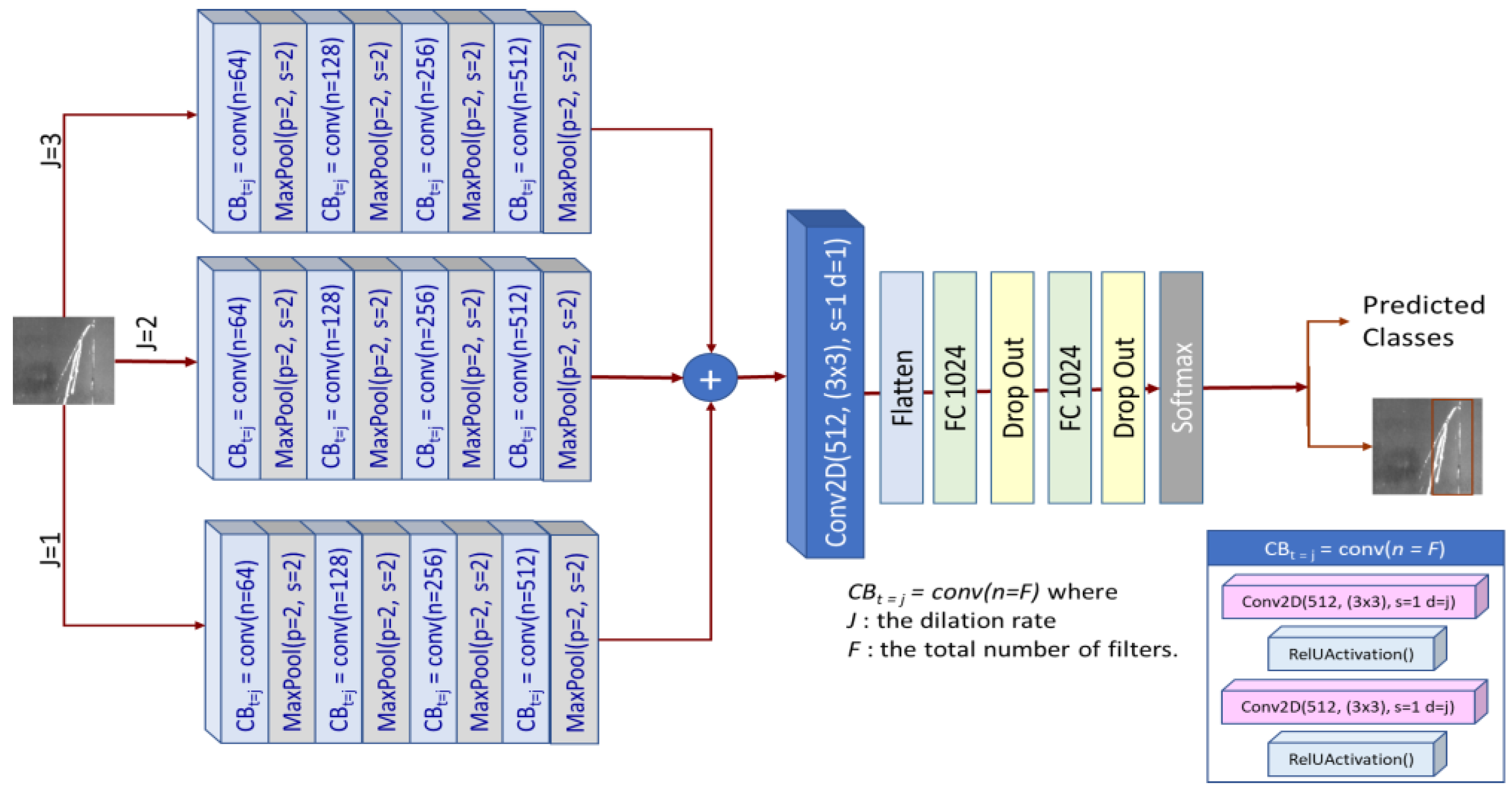
3.2. Proposed DSTEELNet Architecture
3.3. Experiments
3.3.1. Experiment Metrics
3.3.2. Experiment Setup
4. Results and Discussion

| Model | Precision | Recall | F1-score | |||
|---|---|---|---|---|---|---|
| NEU | GNEU | NEU | GNEU | NEU | GNEU | |
| DSTEELNet | 0.961 | 0.97 | 0.957 | 0.97 | 0.956 | 0.97 |
| Vgg16 | 0.91 | 0.92 | 0.882 | 0.89 | 0.884 | 0.89 |
| Vg19 | 0.912 | 0.92 | 0.891 | 0.90 | 0.894 | 0.90 |
| ResNet50 | 0.943 | 0.95 | 0.921 | 0.93 | 0.92 | 0.93 |
| MobileNet | 0.93 | 0.94 | 0.92 | 0.93 | 0.92 | 0.93 |
| Yolov5 | 0.821 | 0.835 | 0.836 | 0.84 | 0.836 | 0.84 |
| Yolov5-SE [69] | 0.879 | 0.882 | 0.887 | 0.89 | 0.886 | 0.89 |
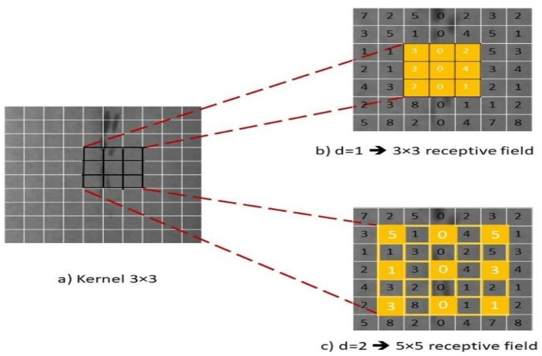
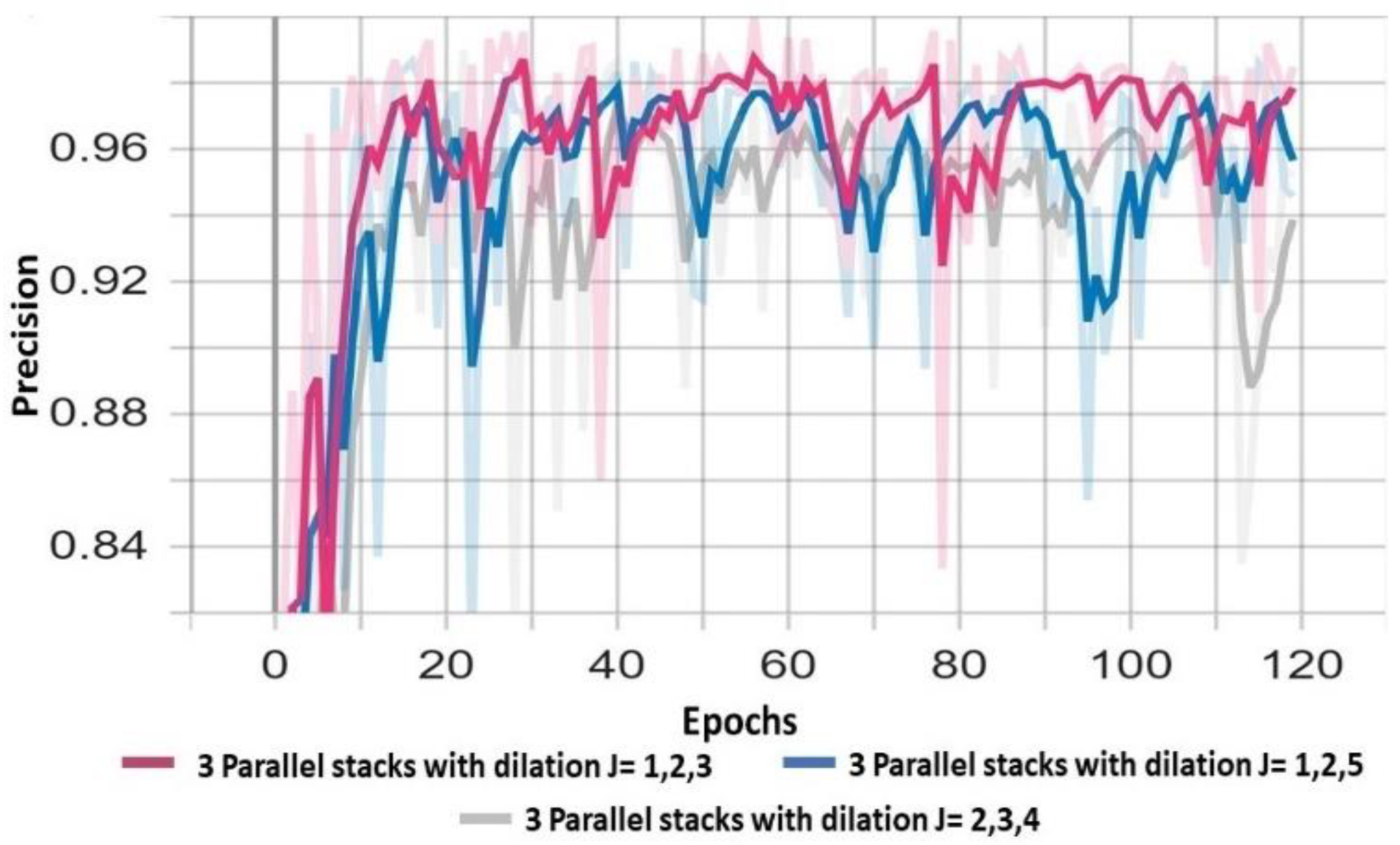
4.1. Dilation Rates Experiments
4.2. Computational Time
5. Conclusions
Funding
Data Availability Statement
Acknowledgments
Conflicts of Interest
Abbreviations
References
- Czimmermann, T.; Ciuti, G.; Milazzo, M.; Chiurazzi, M.; Roccella, S.; Oddo, C.M.; Dario, P. Visual-Based Defect Detection and Classifica-tion Approaches for Industrial Applications—A Survey. Sensors 2020, 20, 5. [Google Scholar] [CrossRef] [PubMed] [Green Version]
- Sadeghi, M.; Soltani, H.; Zamanifar, K. Application of Parallel Algorithm in Image Processing of Steel Surfaces for Defect Detection. Fen Bilim. Derg. (CFD) 2015, 36, 4. [Google Scholar]
- Song, K.; Yan, Y. A noise robust method based on completed local binary patterns for hot-rolled steel strip surface defects. Appl. Surf. Sci. 2013, 285, 858–864. [Google Scholar] [CrossRef]
- Tian, S.; Xu, K. An Algorithm for Surface Defect Identification of Steel Plates Based on Genetic Algo-rithm and Extreme Learning Machine. Metals 2017, 7, 8. [Google Scholar] [CrossRef]
- Ragab, K.; Alsharay, N. Developing Parallel Cracks and Spots Ceramic Defect Detection and Classifica-tion Algorithm Using CUDA. In Proceedings of the EEE 13th International Symposium on Autonomous Decentralized System (ISADS), Bangkok, Thailand, 22–24 March 2017. [Google Scholar]
- Ragab, K. Fast and parallel summed area table for fabric defect detection. Int. J. Pattern Recognit. Artif. Intell. 2016, 30, 9. [Google Scholar] [CrossRef]
- Neogi, N.; Mohanta, D.K.; Dutta, P.K. Review of vision-based steel surface inspection systems. EURASIP J. Image Video Process. 2014, 2014, 50. [Google Scholar] [CrossRef] [Green Version]
- Jia, H.; Murphey, Y.L.; Shi, J.; Chang, T.S. An Intelligent Real-Time Vision System for Surface Defect Detection. In Proceedings of the 17th International Conference on Pattern Recognition, Cambridge, UK, 26 August 2004; IEEE: New York, NY, USA, 2004; Volume 3. [Google Scholar]
- Sager, K.H.; George, L.E. Defect Detection in Fabric Images using Fractal Dimension Approach. In Proceedings of the International Workshop on Advanced Image Technology, Singapore, 6–9 January 2011. [Google Scholar]
- Wang, F.L.; Zuo, B. Detection of surface cutting defect on magnet using Fourier image reconstruction. J. Cent. South Univ. 2016, 23, 1123–1131. [Google Scholar] [CrossRef]
- Zhou, S.; Chen, Y.; Zhang, D.; Xie, J.; Zhou, Y. Classification of surface defects on steel sheet using convolutional neural networks. Mater. Technol. 2017, 51, 123–131. [Google Scholar]
- Wang, H.Y.; Zhang, J.; Tian, Y.; Chen, H.Y.; Sun, H.X.; Liu, K. A Simple Guidance Template-Based Defect Detection Method for Strip Steel Surfaces. IEEE Trans. Ind. Inform. 2018, 15, 2798–2809. [Google Scholar] [CrossRef]
- LeCun, Y.; Bengio, Y.; Hinton, G. Deep learning. Nature 2015, 521, 436–444. [Google Scholar] [CrossRef]
- Ke, X.; Lei, W.; Wang, J. Surface defect recognition of hot-rolled steel plates based on tetrolet trans-form. J. Mech. Eng. 2016, 52, 13–19. [Google Scholar]
- Chu, M.; Gong, R.; Gao, S.; Zhao, J. Steel surface defects recognition based on multi-type statistical features and enhanced twin support vector machine. Chemom. Intell. Lab. Syst. 2017, 171, 130–140. [Google Scholar] [CrossRef]
- Xiao, M.; Jiang, M.; Li, G.; Xie, L.; Yi, L. An evolutionary calssifier for steel surface defects with small sample set. EURASIP J. Image Video Process. 2017, 2017, 48. [Google Scholar] [CrossRef]
- Dong, H.; Song, K.; He, Y.; Xu, J.; Yan, Y.; Meng, Q. PGA-net: Pyramid feature fusion and global context at-tention network for automated surface defect detection. IEEE Trans. Ind. Inform. 2019, 16, 7448–7458. [Google Scholar] [CrossRef]
- Chao, W.; Liu, Y.T.; Yang, Y.N.; Xu, X.Y.; Zhang, T. Research on Classification of Surface Defects of Hot-rolled Steel Strip Based on Deep Learning. DEStech Trans. Comput. Sci. Eng. 2019, 375–379. [Google Scholar] [CrossRef]
- Di, H.; Ke, X.; Peng, Z.; Dongdong, Z. Surface defect classification of steels with a new semi-supervised learning method. Opt. Lasers Eng. 2019, 117, 40–48. [Google Scholar] [CrossRef]
- Krizhevsky, A.; Ilya, S.; Geoffrey, H. ImageNet classification with deep convolutional neural net-works. Commun. ACM 2017, 60, 84–90. [Google Scholar] [CrossRef] [Green Version]
- Liu, S.; Deng, W. Very deep convolutional neural network-based image classification using small training sample size. In Proceedings of the 3rd IAPR Asian Conference on Pattern Recognition (ACPR), Kuala Lumpur, Malaysia, 3–6 November 2015. [Google Scholar]
- Dou, Q.; Chen, H.; Yu, L.; Qin, J.; Heng, P. Multilevel Contextual 3-D CNNs for False Positive Reduction in Pulmonary Nodule Detection. IEEE Trans. Bio-Med. Eng. 2017, 64, 1558–1567. [Google Scholar] [CrossRef]
- Al-masni, M.A.; Kim, D.-H. CMM-Net: Contextual multi-scale multi-level network for efficient biomedi-cal image segmentation. Sci. Rep. 2021, 11, 10191. [Google Scholar] [CrossRef]
- Liang-Chieh, C.; Yi, Y.; Jiang, W.; Wei, X.; Yuille, A.L. Attention to scale: Scale-aware semantic image seg-mentation. In Proceedings of the IEEE Conference on Computer Vision and Pattern Recognition (CVPR), Las Vegas, NV, USA, 27–30 June 2016. [Google Scholar]
- Liu, Y.; Yuan, Y.; Balta, C.; Liu, J. A Light-Weight Deep-Learning Model with Multi-Scale Features for Steel Surface Defect Classification. Materials 2020, 13, 4629. [Google Scholar] [CrossRef]
- Dosovitskiy, A.; Fischer, P.; Ilg, E.; Hausser, P.; Hazirbas, C.; Golkov, V.; Van Der Smagt, P.; Cremers, D.; Brox, T. FlowNet: Learning optical flow with convolutional neural networks. In Proceedings of the IEEE International Conference on Computer Vision (ICCV), Santiago, Chile, 7–13 December 2015. [Google Scholar]
- Chen, L.-C.; Papandreou, G.; Kokkinos, I.; Murphy, K.; Yuille, A.L. DeepLab: Semantic Image Segmenta-tion with Deep Convolutional Nets, Atrous Convolution, and Fully Connected CRFs. IEEE Trans. Pattern Anal. Mach. Intell. 2018, 40, 834–848. [Google Scholar] [CrossRef] [PubMed] [Green Version]
- Ahmed, K.R. Parallel Dilated CNN for Detecting and Classifying Defects in Surface Steel Strips in Re-al-Time. In IntelliSys2021; Lecture Notes in Networks and Systems; Springer: Berlin/Heidelberg, Germany, 2021. [Google Scholar]
- Yu, F.; Koltun, V. Multi-scale context aggregation by dilated convolutions. arXiv 2016, arXiv:1511.07122. [Google Scholar]
- Severstaldataset. Serverstal: Steel Detetction on Kaggle Challenge, Kaggle, 1 March 2021. Available online: https://www.kaggle.com/c/severstal-steel-defect-detection (accessed on 7 November 2022).
- Ren, R.; Hung, T.; Tan, K. A generic deep-learning-based approach for automated surface inspection. IEEE Trans. Cybern. 2018, 48, 929–940. [Google Scholar] [CrossRef] [PubMed]
- Zheng, X.; Zheng, S.; Kong, Y.; Chen, J. Recent advances in surface defect inspection of industrial products using deep learning techniques. Int. J. Adv. Manuf. Technol. 2021, 113, 35–58. [Google Scholar] [CrossRef]
- Gao, Y.; Li, X.; Wang, X.; Wang, L.; Gao, L. A Review on Recent Advances in Vision-based Defect Recog-nition towards Industrial Intelligence. J. Manuf. Syst. 2022, 62, 753–766. [Google Scholar] [CrossRef]
- Taştimur, C.; Karaköse, M.; Akın, E.; Aydın, İ. Rail defect detection and classification with real time im-age processing technique. Int. J. Comput. Sci. Softw. Eng. 2016, 5, 283–290. [Google Scholar]
- Jian, C.; Gao, J.; Ao, Y. Automatic surface defect detection for mobile phone screen glass based on machine vision. Appl. Soft Comput. 2017, 52, 348–358. [Google Scholar] [CrossRef]
- Win, M.; Bushroa, A.; Hassan, M.; Hilman, N.; Ide-Ektessabi, A. A contrast adjustment thresholding method for surface defect detection based on mesoscopy. IEEE Trans. Ind. Inform. 2015, 11, 642–649. [Google Scholar] [CrossRef]
- Kalaiselvi, T.; Nagaraja, P. A rapid automatic brain tumor detection method for MRI images using modi-fied minimum error thresholding technique. Int. J. Imaging Syst. Technol. 2015, 1, 77–85. [Google Scholar]
- Wang, L.; Zhao, Y.; Zhou, Y.; Hao, J. Calculation of flexible printed circuit boards (FPC) global and local defect detection based on computer vision. Circuit World 2016, 42, 49–54. [Google Scholar] [CrossRef]
- Bai, X.; Fang, Y.; Lin, W.; Wang, L.; Ju, B.F. Saliency-based defect detection in industrial images by using phase spectrum. IEEE Trans. Ind. Inform. 2014, 10, 2135–2145. [Google Scholar] [CrossRef]
- Borwankar, R.; Ludwig, R. An Optical Surface Inspection and Automatic Classification Technique Using the Rotated Wavelet Transform. IEEE Trans. Instrum. Meas. 2018, 67, 690–697. [Google Scholar] [CrossRef]
- Hu, G.-H. Automated defect detection in textured surfaces using optimal elliptical Gabor filters. Optik 2015, 126, 1331–1340. [Google Scholar] [CrossRef]
- Susan, S.; Sharma, M. Automatic texture defect detection using Gaussian mixture entropy modeling. Neurocomputing 2017, 239, 232–237. [Google Scholar] [CrossRef]
- Cen, Y.-G.; Zhao, R.-Z.; Cen, L.-H.; Cui, L.-H.; Miao, Z.-J.; Wei, Z. Defect inspection for TFT-LCD images based on the low-rank matrix reconstruction. Neurocomputing 2015, 149, 1206–1215. [Google Scholar] [CrossRef]
- Chondronasios, A.; Popov, I.; Jordanov, I. Feature selection for surface defect classification of extruded aluminum profiles. Int. J. Adv. Manuf. Technol. 2015, 83, 33–41. [Google Scholar] [CrossRef]
- Gibert, X.; Patel, V.M.; Chellappa, R. Deep Multitask Learning for Railway Track Inspection. IEEE Trans. Intell. Transp. Syst. 2016, 18, 153–164. [Google Scholar] [CrossRef] [Green Version]
- Shumin, D.; Zhoufeng, L.; Chunlei, L. Adaboost learning for fabric defect detection based on hog and SVM. In Proceedings of the International Conference on Multimedia Technology, Hangzhou, China, 26–28 July 2011. [Google Scholar]
- Ahmed, K.R.; Al-Saeed, M.; Al-Jumah, M.I. Parallel Algorithms to detect and classify defects in Surface Steel Strips. In Proceedings of the World Congress in Computer Science, Computer Engineering, and Applied Computing (CSCE’20), Las Vegas, NV, USA, 27–30 July 2020. [Google Scholar]
- Masci, J.; Meier, U.; Fricout, G.; Schmidhuber, J. Multi-scale pyramidal pooling network for generic steel de-fect classification. In Proceedings of the International Joint Conference on Neural Networks, Dallas, TX, USA, 4–9 August 2013; pp. 1–8. [Google Scholar]
- Natarajan, V.; Hung, T.-Y.; Vaikundam, S.; Chia, L.-T. Convolutional networks for voting-based anomaly classification in metal surface inspection. In Proceedings of the IEEE International Conference on Industrial Technology (ICIT), Toronto, ON, Canada, 22–25 March 2017. [Google Scholar]
- He, Y.S.K.; Meng, Q.; Yan, Y. An End-to-End Steel Surface Defect Detection Approach via Fusing Multi-ple Hierarchical Features. IEEE Trans. Instrum. Meas. 2020, 69, 1493–1504. [Google Scholar] [CrossRef]
- Tao, X.; Zhang, D.; Ma, W.; Liu, X.; Xu, D. Automatic Metallic Surface Defect Detection and Recognition with Convolutional Neural Networks. Appl. Sci. 2018, 8, 1575. [Google Scholar] [CrossRef] [Green Version]
- He, K.; Zhang, X.; Ren, S.; Sun, J. Deep Residual Learning for Image Recognition. In Proceedings of the IEEE Conference on Computer Vision and Pattern Recognition (CVPR), Las Vegas, NV, USA, 27–30 June 2016. [Google Scholar]
- Wang, T.; Chen, Y.; Qiao, M.; Snoussi, H. A fast and robust convolutional neural network-based defect detection model in product quality control. Int. J. Adv. Manuf. Technol. 2018, 94, 3465–3471. [Google Scholar] [CrossRef]
- Cha, Y.-J.; Choi, W.; Suh, G.; Mahmoudkhani, S.; Büyüköztürk, O. Autonomous structural visual inspection using region—Based deep learning for detecting multiple damage types. Comput.-Aided Civ. Infrastruct. Eng. 2018, 33, 731–747. [Google Scholar] [CrossRef]
- Ren, S.; He, K.; Girshick, R.; Sun, J. Faster R-CNN: Towards Real-Time Object Detection with Region Pro-posal Networks. IEEE Trans. Pattern Anal. Mach. Intell. 2017, 6, 1137–1149. [Google Scholar] [CrossRef] [PubMed] [Green Version]
- Zhao, W.; Chen, F.; Huang, H.; Li, D.; Cheng, W. A New Steel Defect Detection Algorithm Based on Deep Learning. Comput. Intell. Neurosci. 2021, 2021, 5592878. [Google Scholar] [CrossRef] [PubMed]
- Yan, J.; Wang, H.; Yan, M. IoU-adaptive deformable R-CNN: Make full use of IoU for multi-class object detection in remote sensing imagery. Remote Sens. 2019, 11, 286. [Google Scholar] [CrossRef] [Green Version]
- Li, Z.; Tian, X.; Liu, X.; Liu, Y.; Shi, X. A Two-Stage Industrial Defect Detection Framework Based on Im-proved-YOLOv5 and Optimized-Inception-ResnetV2 Models. Appl. Sci. 2022, 12, 834. [Google Scholar] [CrossRef]
- Ian, J.G.; Jean, P.-A.; Mehdi, M.; Bing, X.; David, W.-F.; Sherjil, O.; Aaron, C.; Yoshua, B. Generative Adver-sarial Networks. arXiv 2014, arXiv:1406.2661. [Google Scholar]
- Radford, A.; Metz, L.; Chintala, S. Unsupervised Representation Learning with Deep Convolu-tional Generative Adversarial Networks. arXiv 2016, arXiv:1511.06434. [Google Scholar]
- Luo, W.; Li, Y.; Urtasun, R.; Zemel, R. Understanding the effective receptive field in deep convolutional neural networks. arXiv 2017, arXiv:1701.04128. [Google Scholar]
- Xiang, W.; Zhang, D.-Q.; Yu, H.; Athitsos, V. Context-Aware Single-Shot Detector. In Proceedings of the IEEE Winter Confer-ence on Applications of Computer Vision (WACV), Lake Tahoe, NV, USA, 12–15 March 2018. [Google Scholar]
- Chen, L.-C.; Papandreou, G.; Kokkinos, I.; Murphy, K.; Yuille, A.L. Semantic image segmentation with deep convolutional nets and fully connected CRFs. In Proceedings of the International Conference on Learninig Representations (ICLR2015), San Diego, CA, USA, 7–9 May 2015. [Google Scholar]
- Panqu, W.; Pengfei, C.; Ye, Y.; Ding, L.; Zehua, H.; Xiaodi, H.; Garrison, C. Understanding Convolution for Semantic Segmentation. In Proceedings of the 2018 IEEE Winter Conference on Applications of Computer Vision (WACV), Lake Tahoe, NV, USA, 12–15 March 2018. [Google Scholar]
- Scherer, D.; Müller, A.; Behnke, S. Evaluation of Pooling Operations in Convolutional Architectures for Object Recognition. In Proceedings of the 20th International Conference on Artificial Neural Networks—ICANN 2010, Thessaloniki, Greece, 15–18 September 2010. [Google Scholar]
- Liu, B.; Zhang, X.; Gao, Z.; Chen, L. Weld defect images classification with VGG16-Based neural network. In Proceedings of the International Forum on Digital TV and Wireless Multimedia Communications (IFTC 2017), Shanghai, China, 8–9 November 2017. [Google Scholar]
- Howard, A.G.; Zhu, M.; Chen, B.; Kalenichenko, D.; Wang, W.; Weyand, T.; Andreetto, M.; Adam, H. Mo-bilenets: Efficient convo- lutional neural networks for mobile vision applications. arXiv 2017, arXiv:1704.04861. [Google Scholar]
- Jocher, G. “Yolov5,” LIC, Ultralytics. 2020. Available online: https://github.com/ultralytics/yolov5 (accessed on 12 January 2021).
- Zeqiang, S.; Bingcai, C. Improved Yolov5 Algorithm for Surface Defect Detection of Strip Steel. In Artificial Intelligence in China; Springer: Singapore, 2022; Volume 854, pp. 448–456. [Google Scholar]
- Kingma, D.P.; Ba, L.J. Adam: A Method for Stochastic Optimization. In Proceedings of the International Conference on Learn-ing Representations (ICLR), San Diego, CA, USA, 7–9 May 2015. [Google Scholar]
- Lv, X.; Duan, F.; Jiang, J.J.; Fu, X.; Gan, L. Deep Metallic Surface Defect Detection: The New Bench-mark and Detection Network. Sensors 2020, 20, 1562. [Google Scholar]


| Parameters | Value |
|---|---|
| Height Shift | 0.08 |
| Width Shift | 0.08 |
| Rotation Range | 8 |
| Fill mode | Nearest |
| Zoom Range | 0.08 |
| Shear Range | 0.3 |
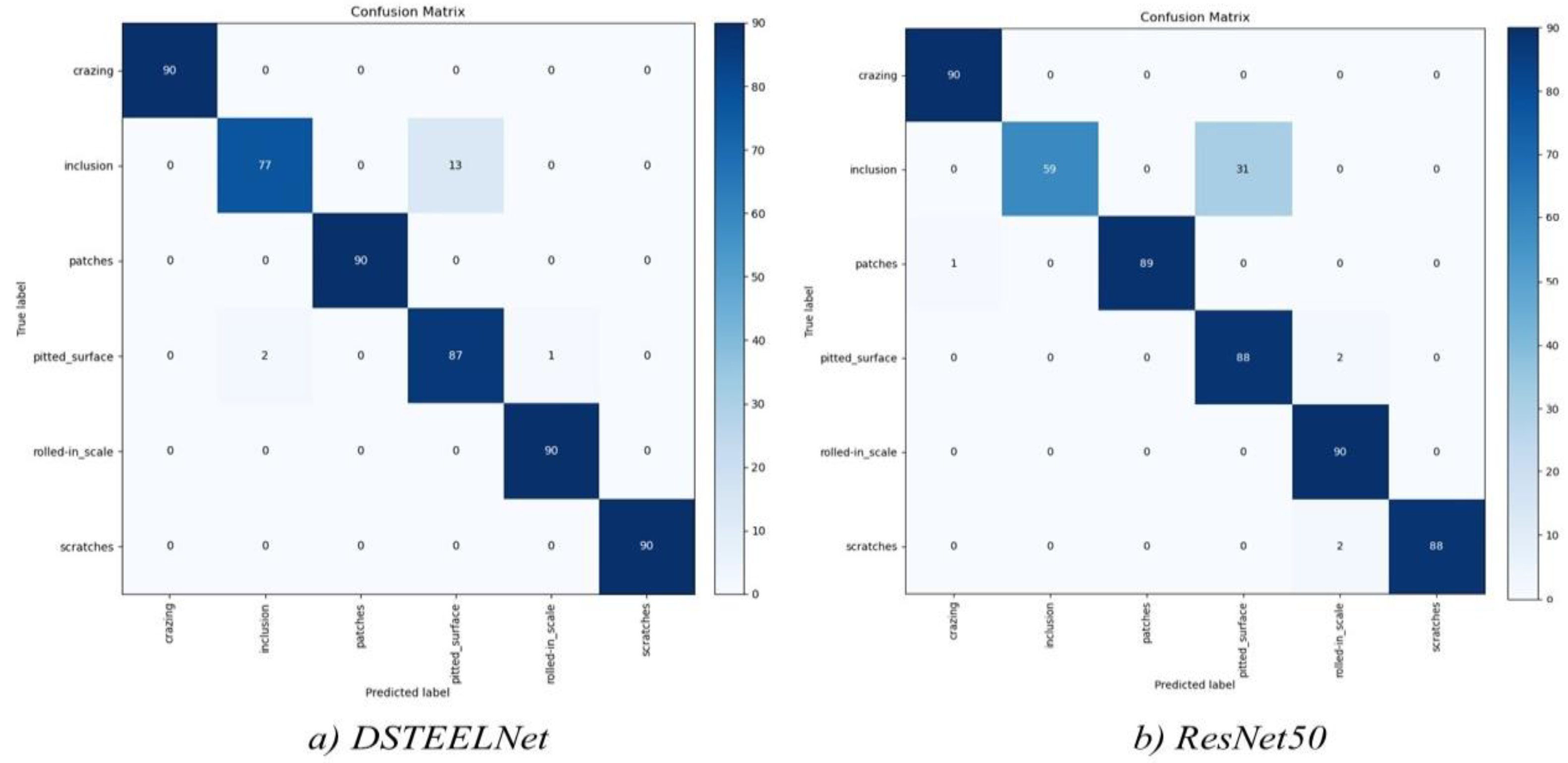
| DSTEELNet | VGG16 | VGG19 | Resnet50 | MobileNet | |||||||||||
|---|---|---|---|---|---|---|---|---|---|---|---|---|---|---|---|
| Precision | Recall | F1 | Precision | Recall | F1 | Precision | Recall | F1 | Precision | Recall | F1 | Precision | Recall | F1 | |
| Crazing | 1.00 | 1.00 | 1.00 | 1.00 | 1.00 | 1.00 | 0.95 | 1.00 | 0.97 | 0.99 | 1.00 | 0.99 | 0.98 | 1.00 | 0.99 |
| Inclusion | 0.97 | 0.86 | 0.91 | 1.00 | 0.51 | 0.68 | 0.94 | 0.54 | 0.69 | 1.00 | 0.66 | 0.79 | 1.00 | 0.82 | 0.82 |
| Patches | 1.00 | 1.00 | 1.00 | 0.89 | 1.00 | 0.94 | 1.00 | 0.98 | 0.99 | 1.00 | 0.99 | 0.99 | 1.00 | 0.99 | 0.99 |
| Pitted_surface | 0.87 | 0.97 | 0.92 | 0.66 | 0.97 | 0.79 | 0.67 | 0.89 | 0.76 | 0.74 | 0.98 | 0.84 | 0.73 | 0.98 | 0.84 |
| Rolled-in_Scale | 0.99 | 1.00 | 0.99 | 0.96 | 1.00 | 0.98 | 0.94 | 1.00 | 0.97 | 0.96 | 1.00 | 0.98 | 0.98 | 0.90 | 0.94 |
| Scratches | 1.00 | 1.00 | 1.00 | 1.00 | 0.87 | 0.93 | 1.00 | 0.99 | 0.99 | 1.00 | 0.98 | 0.99 | 0.96 | 1.00 | 0.98 |
| mAP | 0.972 | 0.912 | 0.90 | 0.93 | 0.94 | ||||||||||
| Defect | DSTEELNet | Yolov5 | Yolov5-SE |
|---|---|---|---|
| Crazing | 1.00 | 0.84 | 0.90 |
| Inclusion | 0.97 | 0.86 | 0.88 |
| Patches | 1.00 | 0.92 | 0.94 |
| Pitted surface | 0.87 | 0.89 | 0.99 |
| Rolled-in scale | 1.00 | 0.52 | 0.64 |
| Scratches | 0.99 | 0.98 | 1.00 |
| Model | Precision | Accuracy | F1-score |
|---|---|---|---|
| DSTEELNet | 0.96 | 0.96 | 0.96 |
| Vgg16 | 0.91 | 0.90 | 0.89 |
| Vgg19 | 0.91 | 0.91 | 0.90 |
| ResNet50 | 0.93 | 0.93 | 0.932 |
| MobileNet | 0.94 | 0.926 | 0.93 |
| DSTEELNet | Precision | Recall | F1-score | |
|---|---|---|---|---|
| One Stack | dilation 1,1,2,2,3 | 0.93 | 0.93 | 0.93 |
| dilation 1,2,3,4,5 | 0.89 | 0.90 | 0.90 | |
| 3-parallel stacks | J = 1,2,3 | 0.96 | 0.958 | 0.957 |
| J = 2,3,4 | 0.92 | 0.91 | 0.91 | |
| J = 1,2,5 | 093 | 0.92 | 0.92 | |
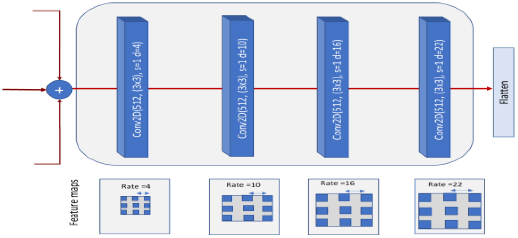
| J = 1,2,3+ ASPP(4,10,16,22) | DSTEELNet-ASPP | |||
| 0.98 | 0.98 | 0.98 | ||
| Traditional Techniques | Deep Learning Techniques | |||||||
|---|---|---|---|---|---|---|---|---|
| HOG-SVM | LBP-SVM | GLCM- SVM | Vgg16 | Vgg19 | ResNet50 | MobileNet | DSTEELNet | Yolov5 |
| 443.5 | 382.3 | 454.57 | 29 | 31 | 36 | 30 | 23 | 24 |
Disclaimer/Publisher’s Note: The statements, opinions and data contained in all publications are solely those of the individual author(s) and contributor(s) and not of MDPI and/or the editor(s). MDPI and/or the editor(s) disclaim responsibility for any injury to people or property resulting from any ideas, methods, instructions or products referred to in the content. |
© 2023 by the author. Licensee MDPI, Basel, Switzerland. This article is an open access article distributed under the terms and conditions of the Creative Commons Attribution (CC BY) license (https://creativecommons.org/licenses/by/4.0/).
Share and Cite
Ahmed, K.R. DSTEELNet: A Real-Time Parallel Dilated CNN with Atrous Spatial Pyramid Pooling for Detecting and Classifying Defects in Surface Steel Strips. Sensors 2023, 23, 544. https://doi.org/10.3390/s23010544
Ahmed KR. DSTEELNet: A Real-Time Parallel Dilated CNN with Atrous Spatial Pyramid Pooling for Detecting and Classifying Defects in Surface Steel Strips. Sensors. 2023; 23(1):544. https://doi.org/10.3390/s23010544
Chicago/Turabian StyleAhmed, Khaled R. 2023. "DSTEELNet: A Real-Time Parallel Dilated CNN with Atrous Spatial Pyramid Pooling for Detecting and Classifying Defects in Surface Steel Strips" Sensors 23, no. 1: 544. https://doi.org/10.3390/s23010544