
Non-Invasive In Vivo Estimation of HbA1c Using Monte Carlo Photon Propagation Simulation: Application of Tissue-Segmented 3D MRI Stacks of the Fingertip and Wrist for Wearable Systems


Abstract
:1. Introduction
- We have used a novel composite tissue material model derived from MR images and Monte Carlo simulations with multiple source signals to minimize the estimation errors;
- The proposed the wrist model with multiple light-emitting diodes (LEDs) and a single PD exhibited the highest correlation with the reference experimental data among the three tested models;
- Establishing our HbA1c estimation method can greatly improve the use of mobile-camera-based PPG sensors for the accurate estimation of the HbA1c values, thereby resulting in low-cost diagnostic devices.
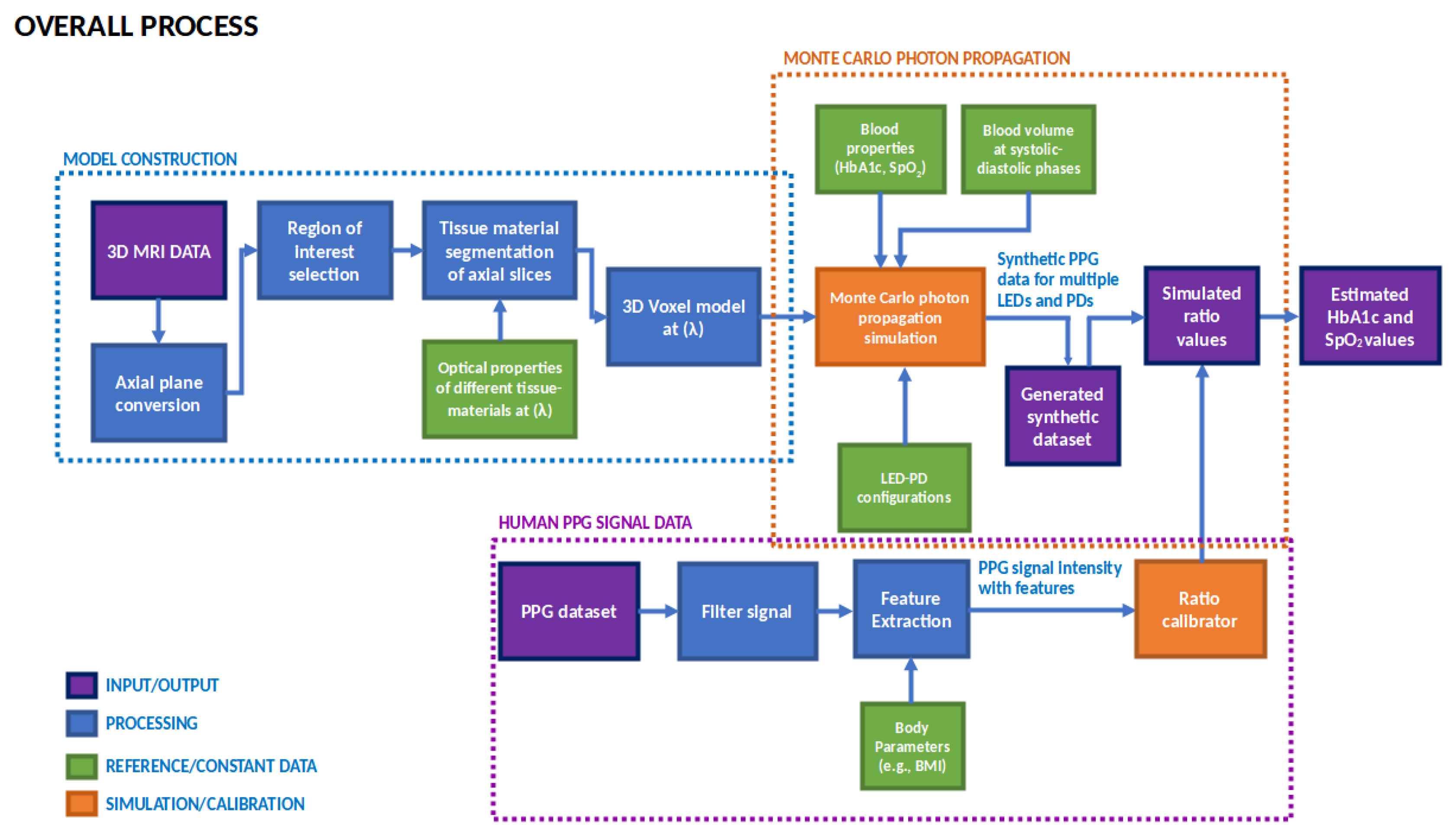
2. Methodology
2.1. Monte Carlo Photon Propagation
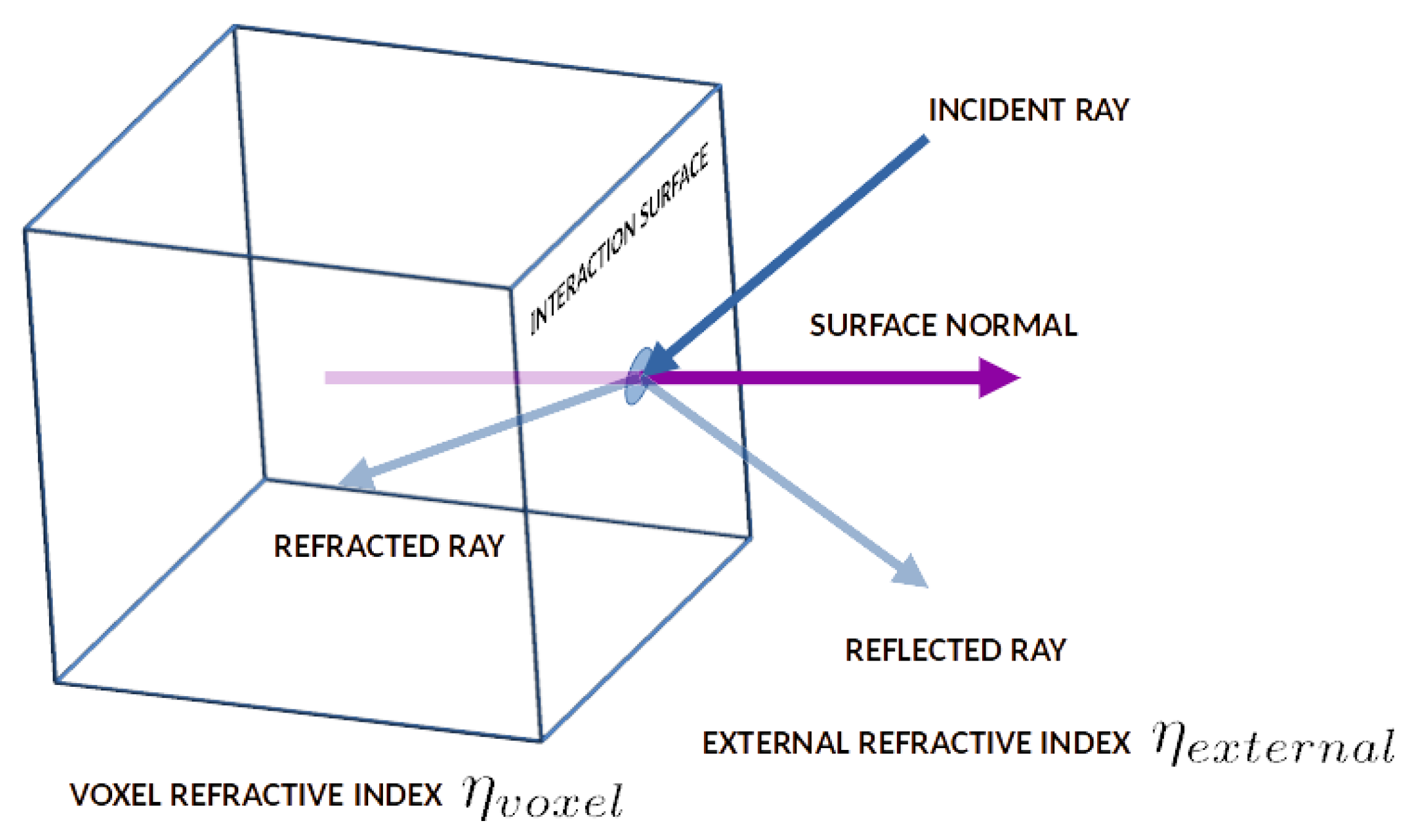
2.1.1. Photon Propagation Theory
| Algorithm 1: Pseudocode of the Monte Carlo photon propagation process | |
| 1 2 3 4 5 6 7 8 9 10 11 12 13 14 15 16 17 18 19 20 21 22 23 24 25 26 27 | Initialize:system_variables, voxel_model, total_photon_number, photon_data for total_photon_number: photon <= generatePhotonPacket(photon_location, photon_direction) while photon.weight > 0 and photon.is_out == False: tissue_type<= calculateTissueMedium(photon) step <= calculateStepSize(tissue_type) movePhoton(photon) if photonCrossedTissueBoundary(photon): r <= calculateReflectionCoefficient(photon) R <= calculatePowerReflectionCoefficient(r) photon <= reflect_refractPhoton(photon, R) endif absorbPhotonWeight(photon) recordPhotonData(photon) scatterPhoton(photon) if photon.weight < roulette_cutoff: photon <= photonRoulette(photon) endif endwhile endfor |
2.1.2. Image-Stack-Based Calculation Method
2.1.3. Composite Tissue Material Generation
2.1.4. Time-Resolved Photon Transport
2.2. Model Construction
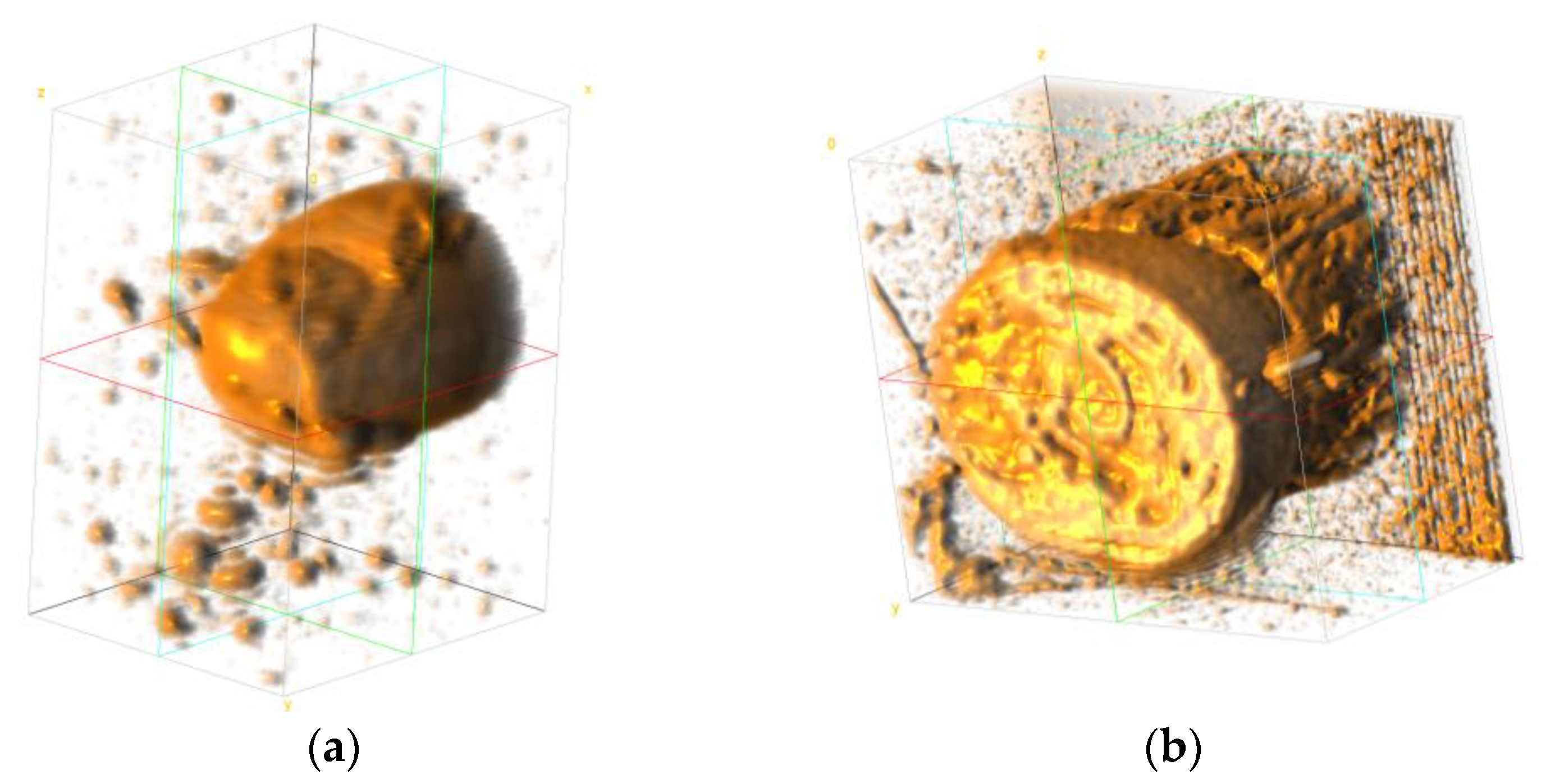
2.2.1. MR Image Data
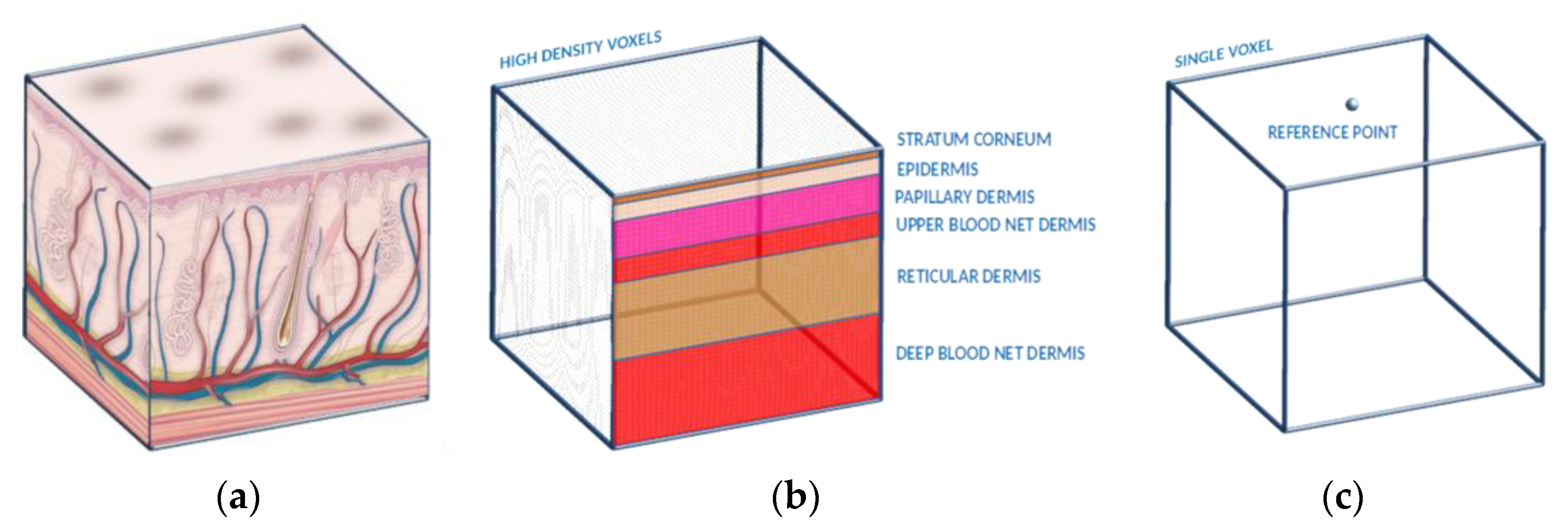
2.2.2. Tissue Types
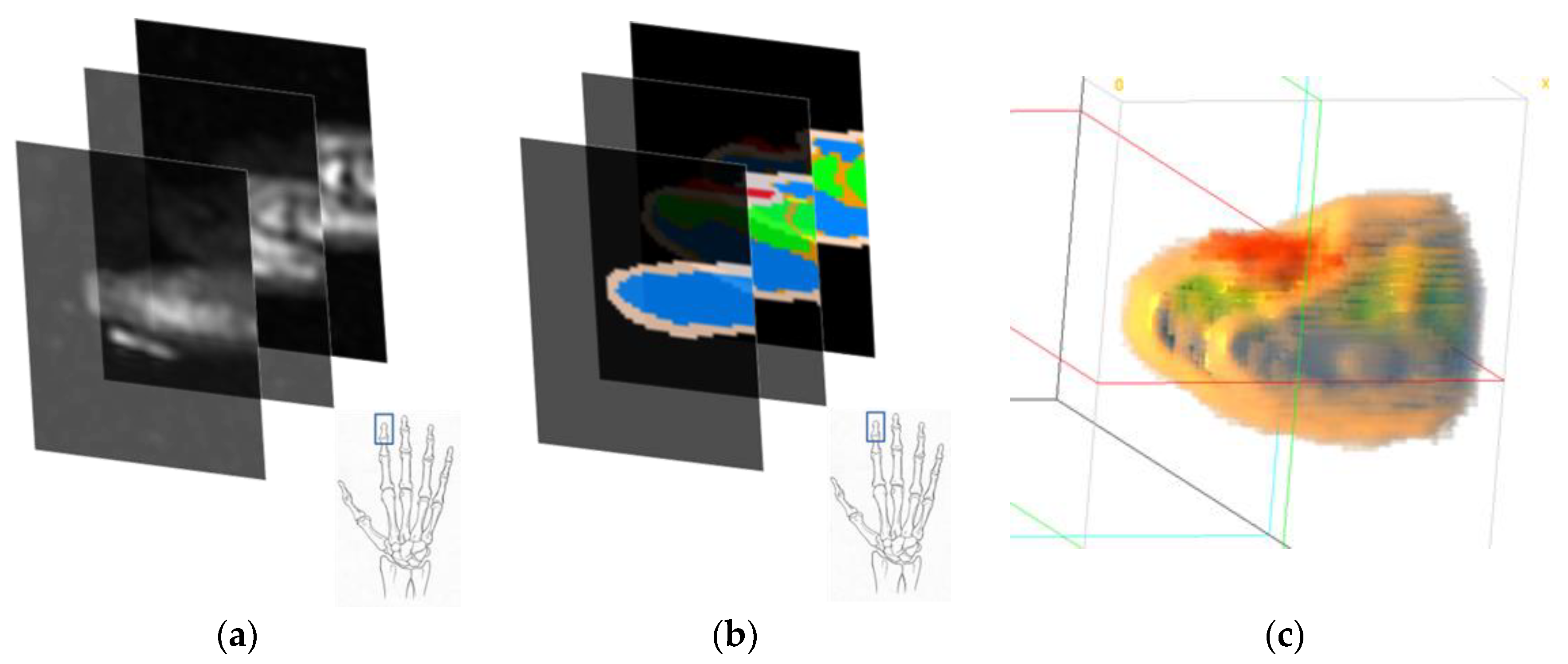
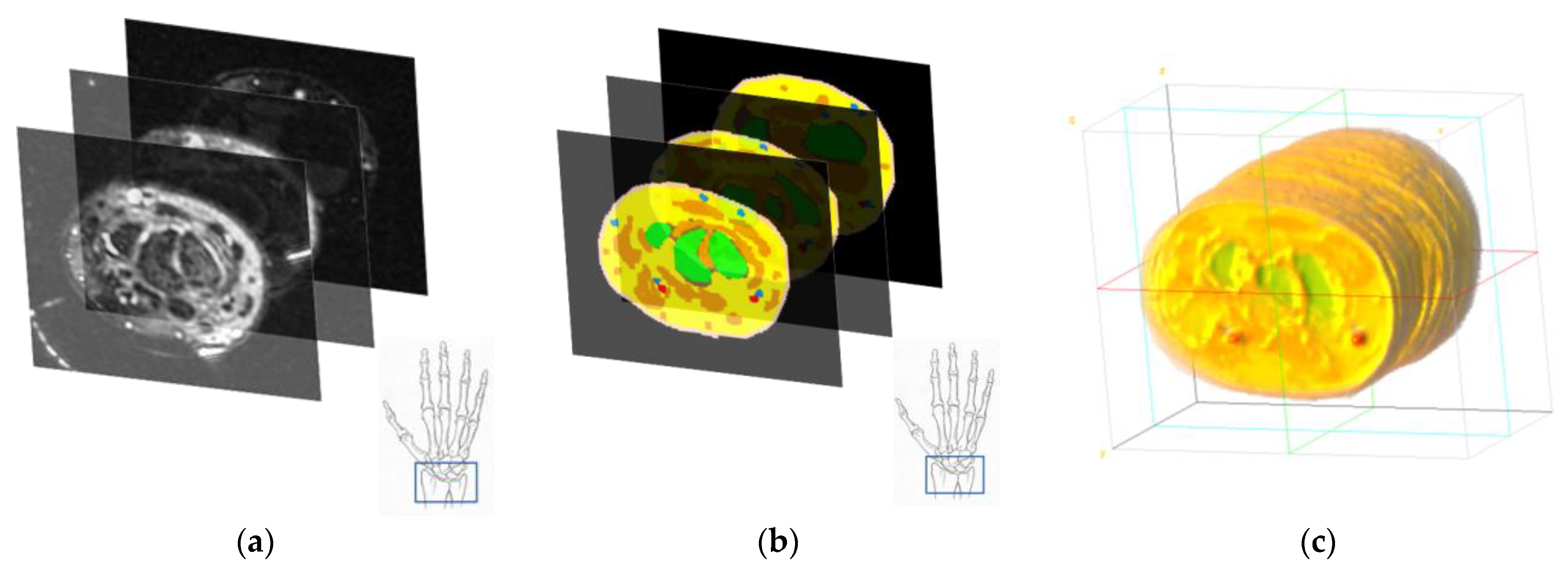
2.2.3. Segmentation
Fingertip
Wrist
2.3. System Configuration
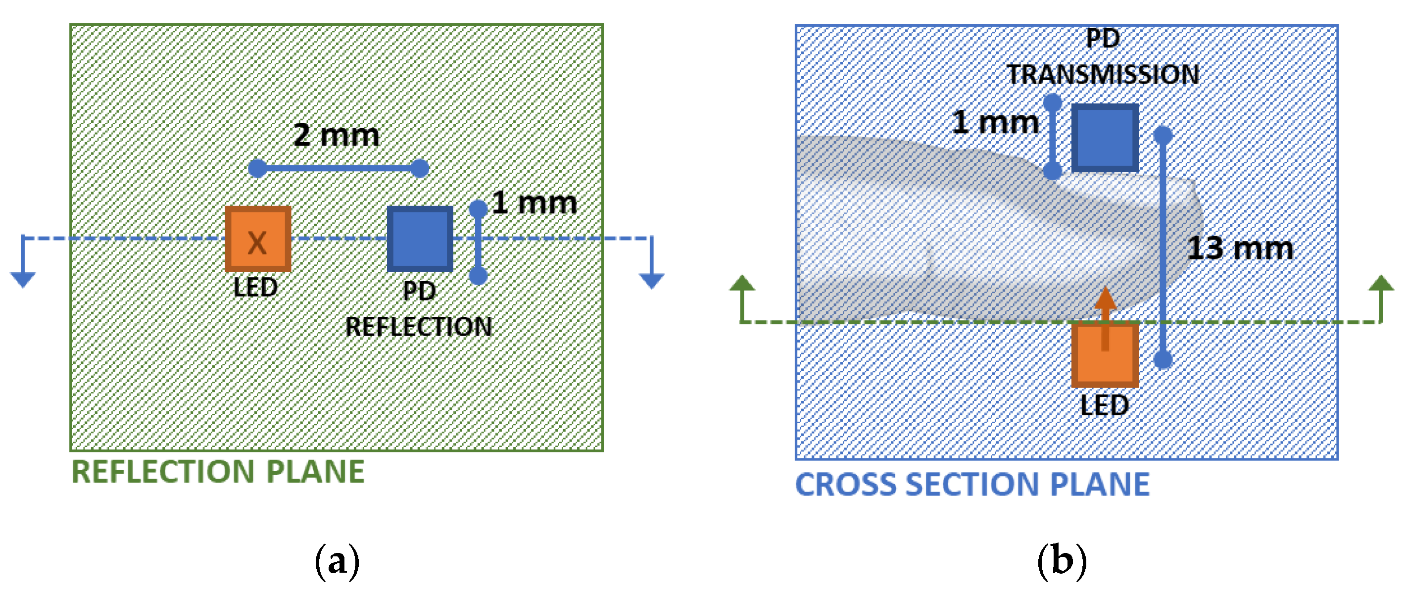
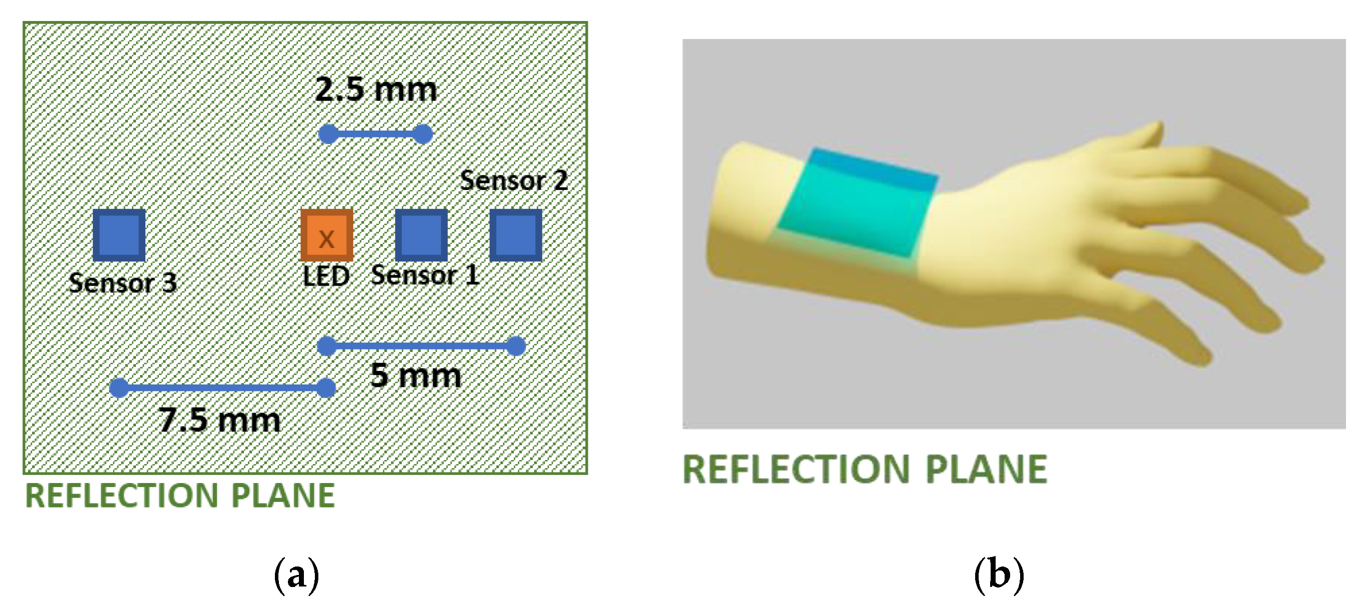
2.3.1. Source–Receiver Properties
2.3.2. Source–Receiver Placement Configurations
2.4. Calibration
3. Results
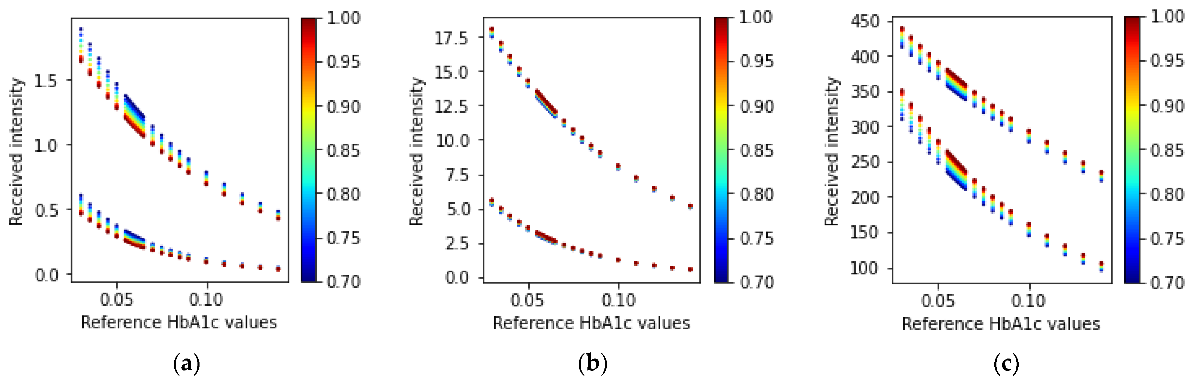
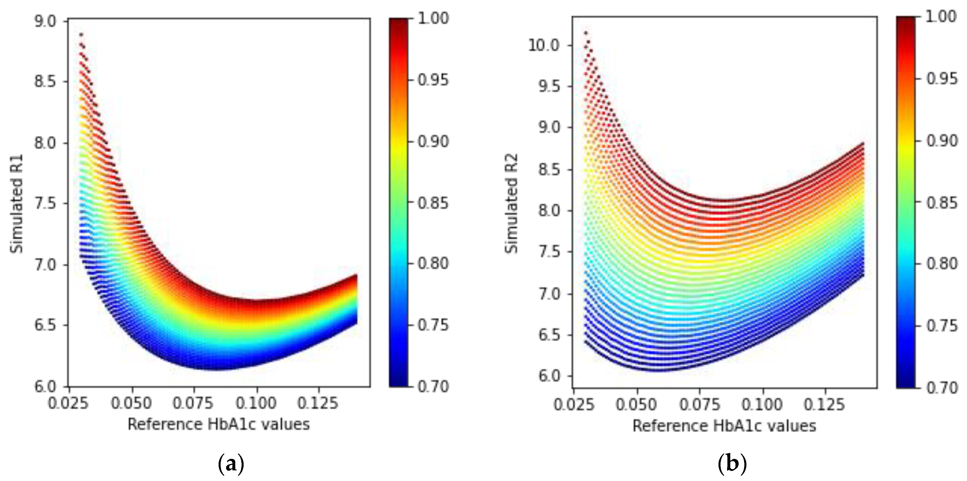
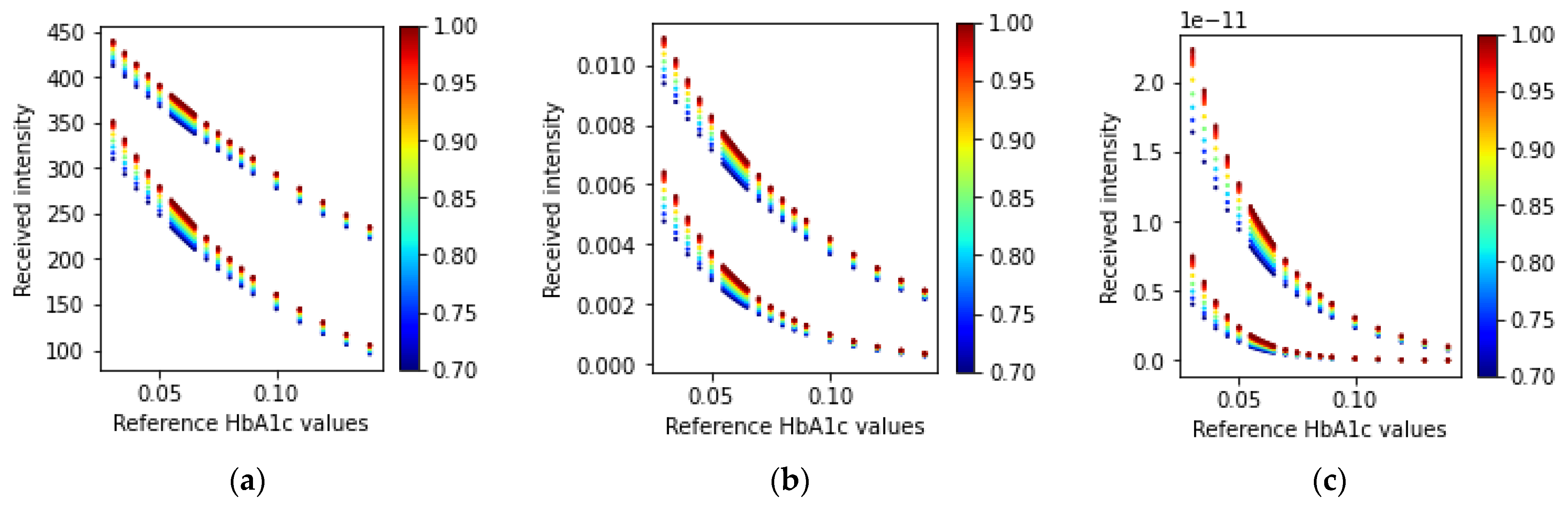
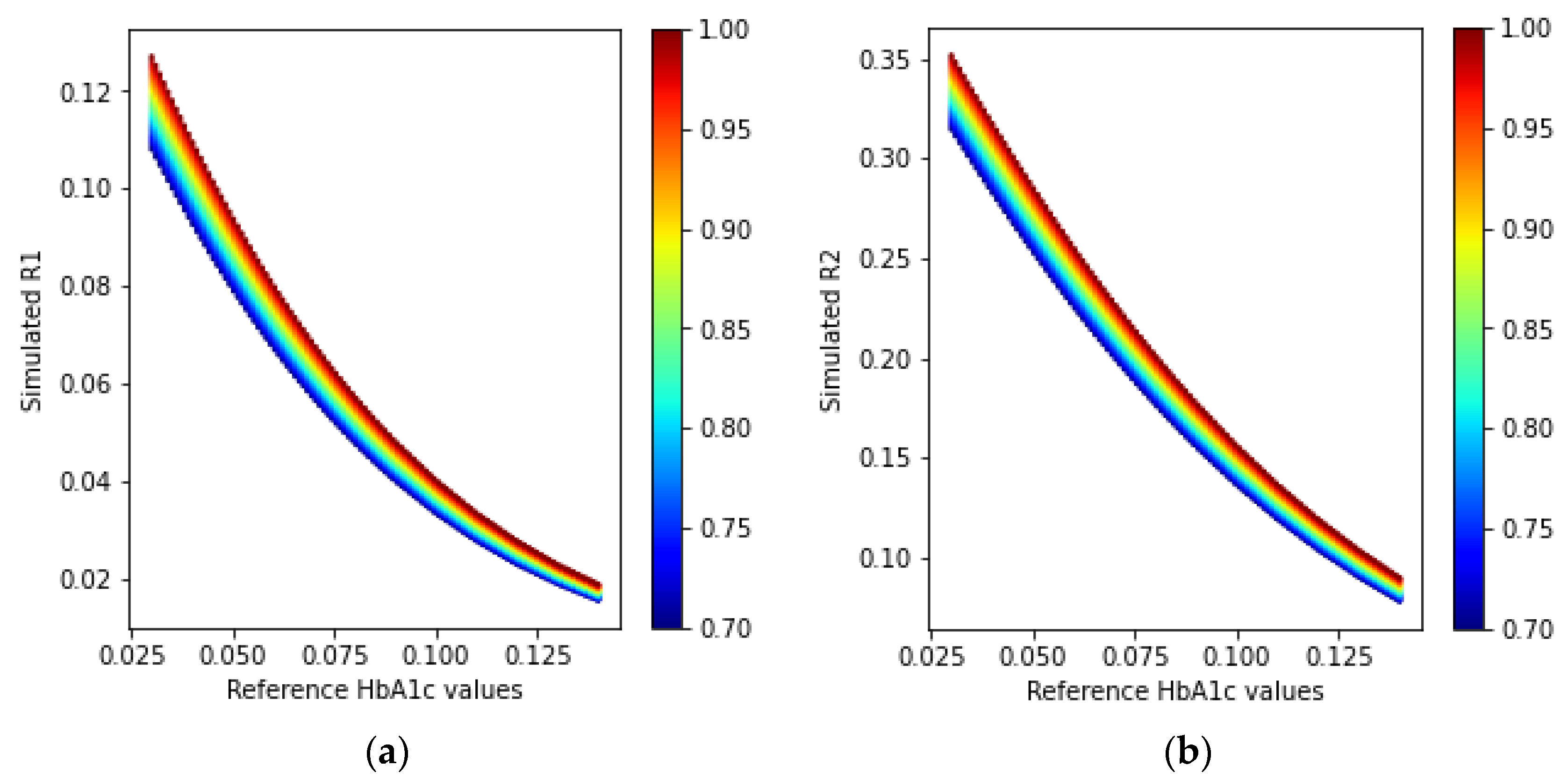
3.1. Simulation Results
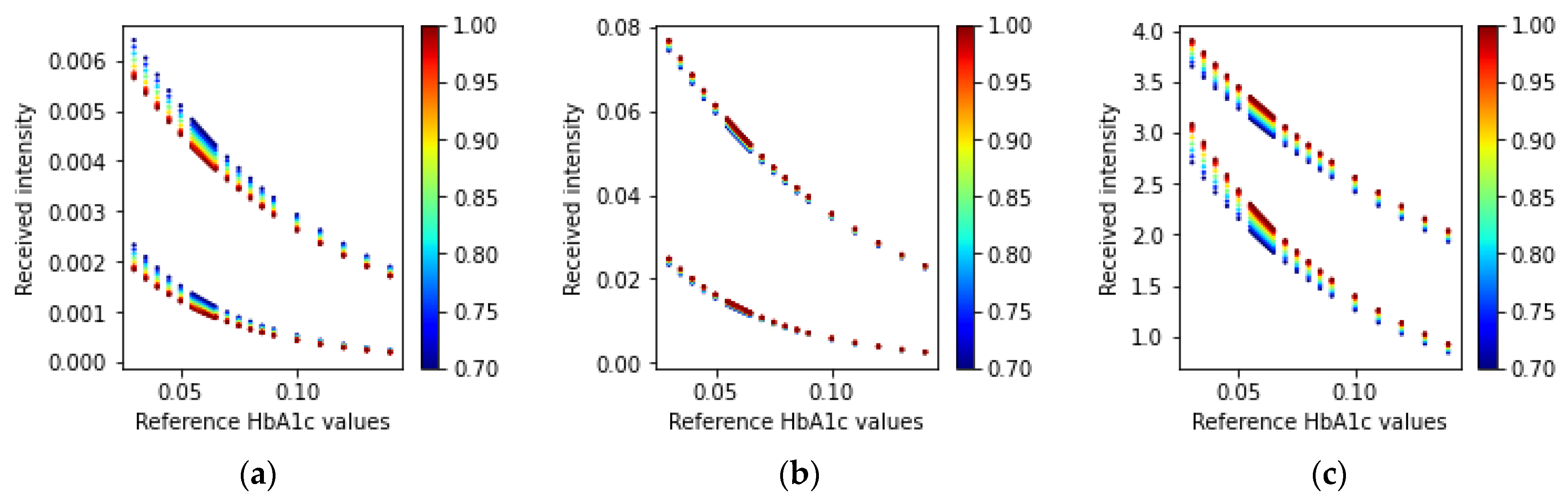
3.1.1. Fingertip: Transmission-Type
3.1.2. Fingertip: Reflection-Type
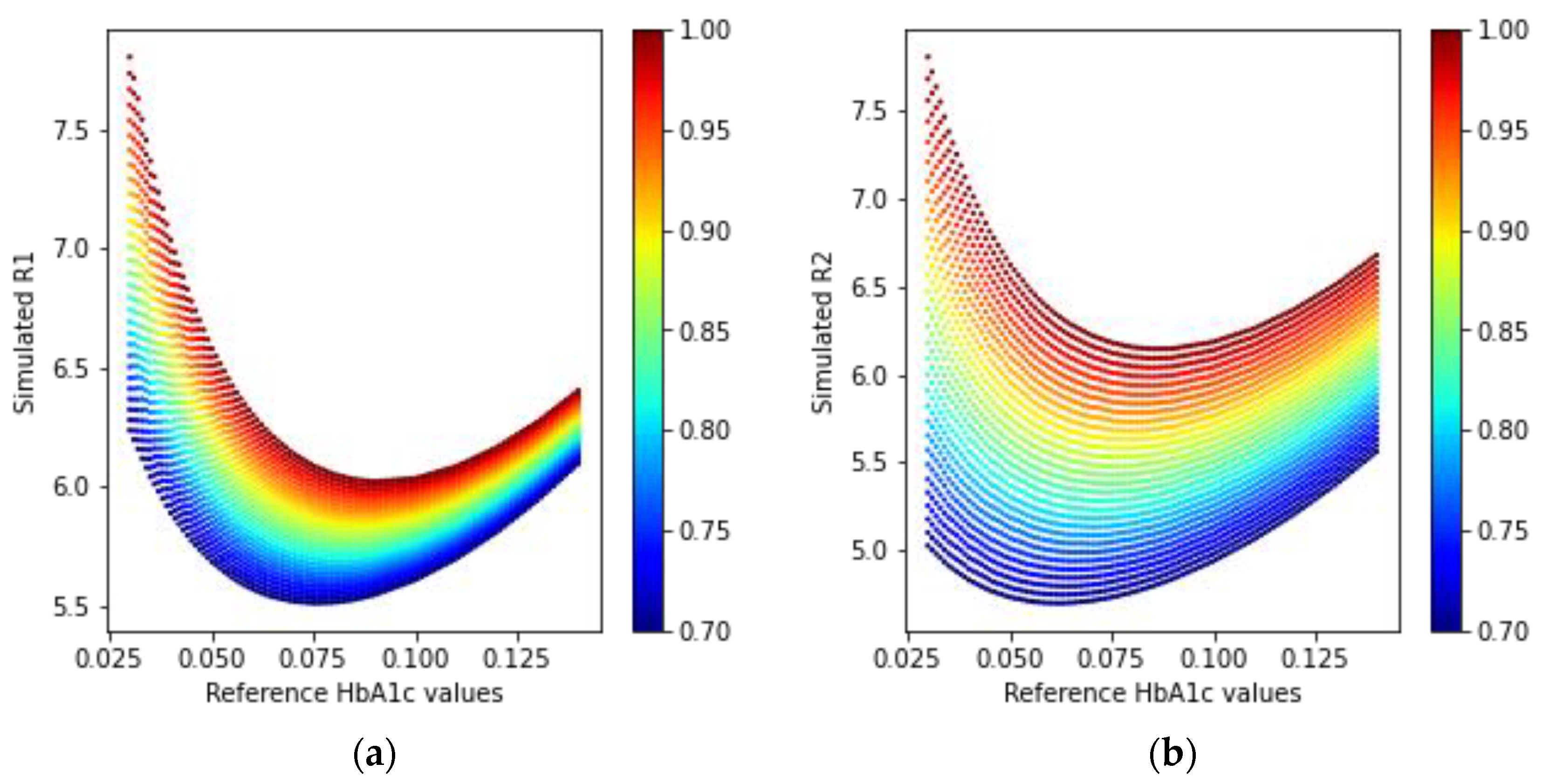
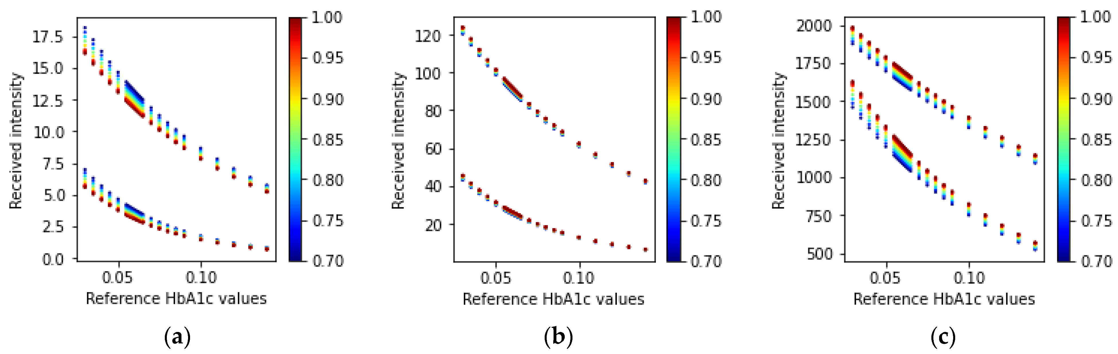
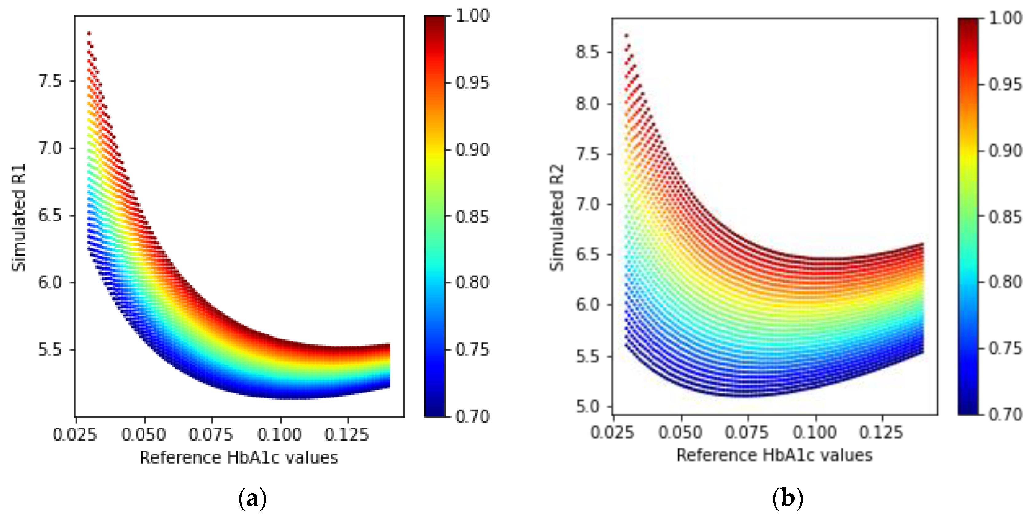
3.1.3. Wrist: One PD and Multiple Wavelength LEDs
3.1.4. Wrist: Multiple PDs and One Wavelength LED
3.2. Human Data Demographics
3.3. Model Validation Results
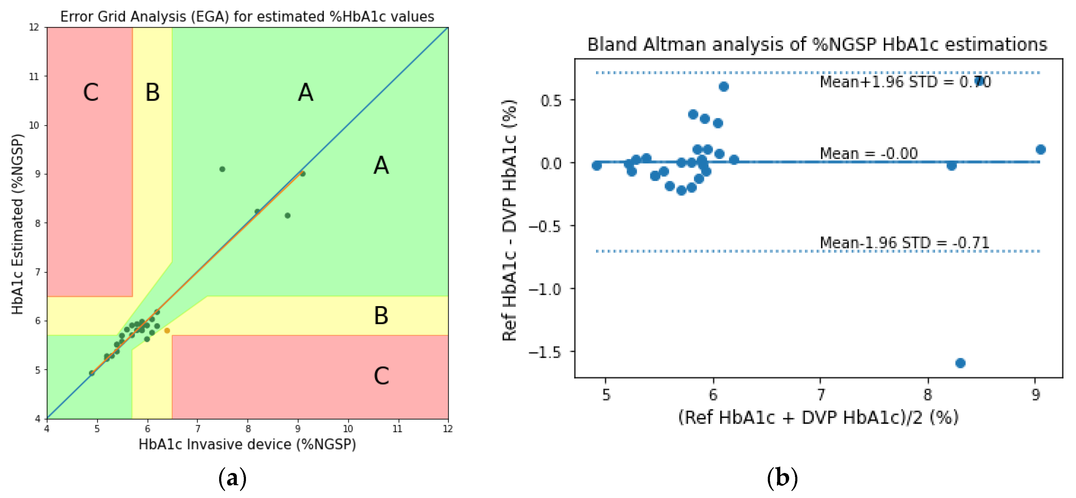
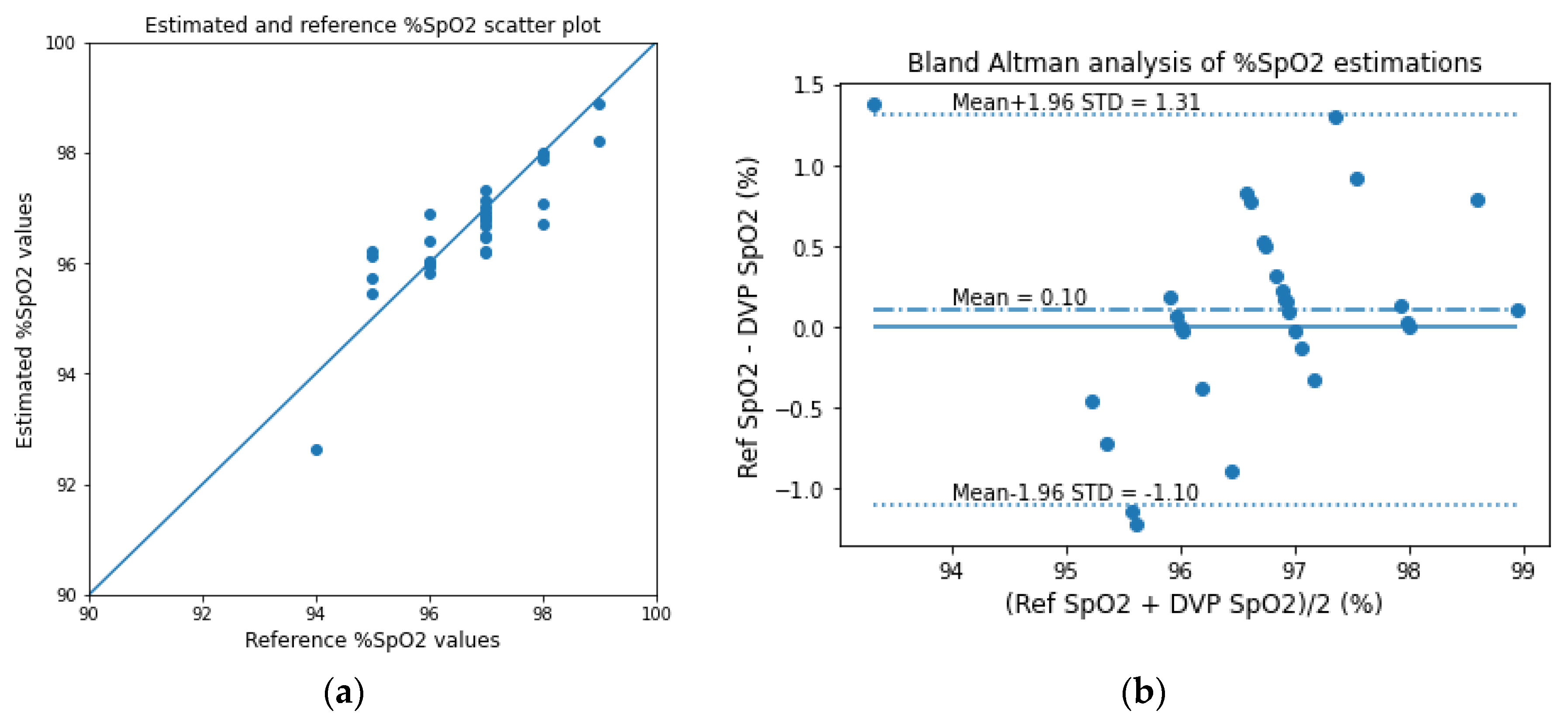
3.3.1. Fingertip: Transmission-Type
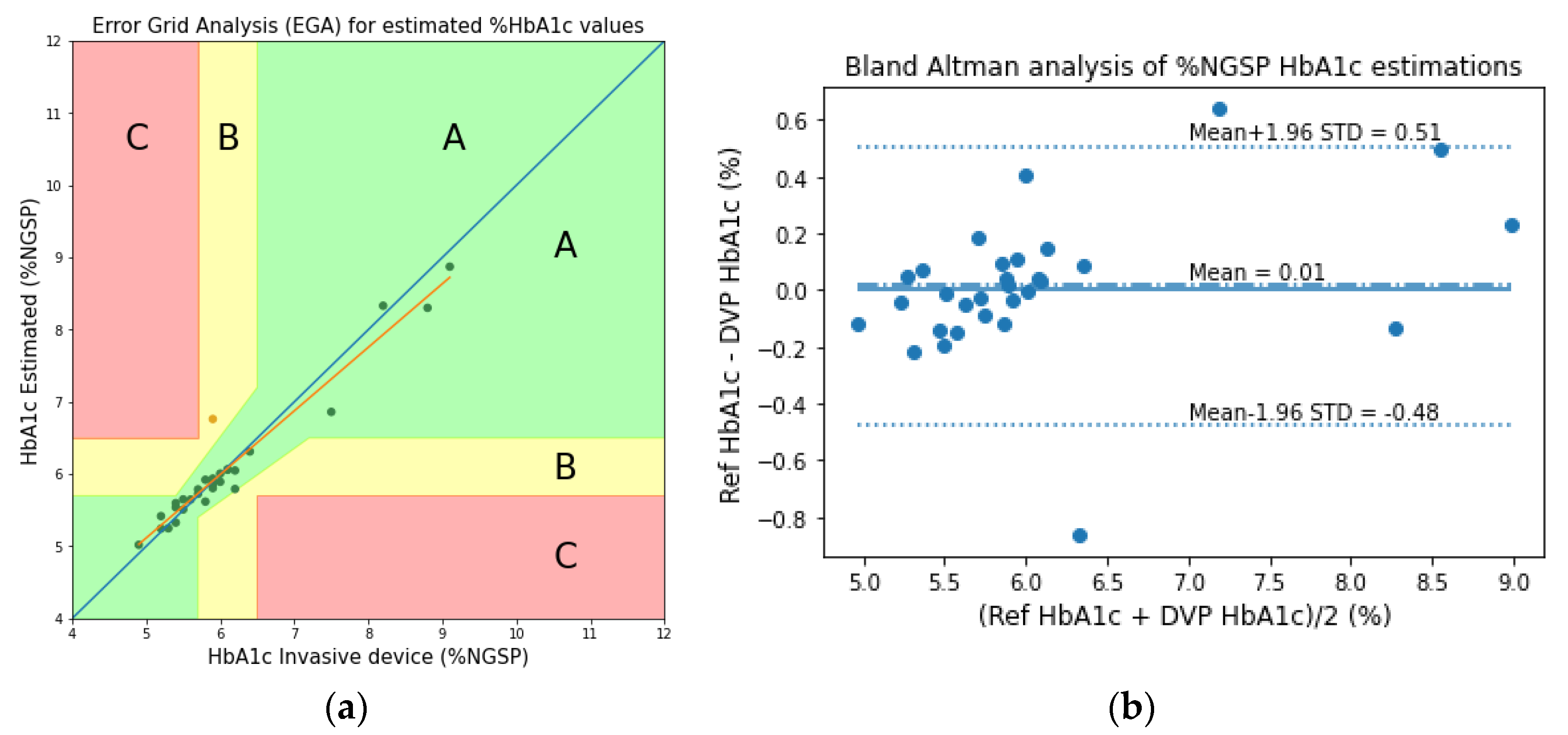
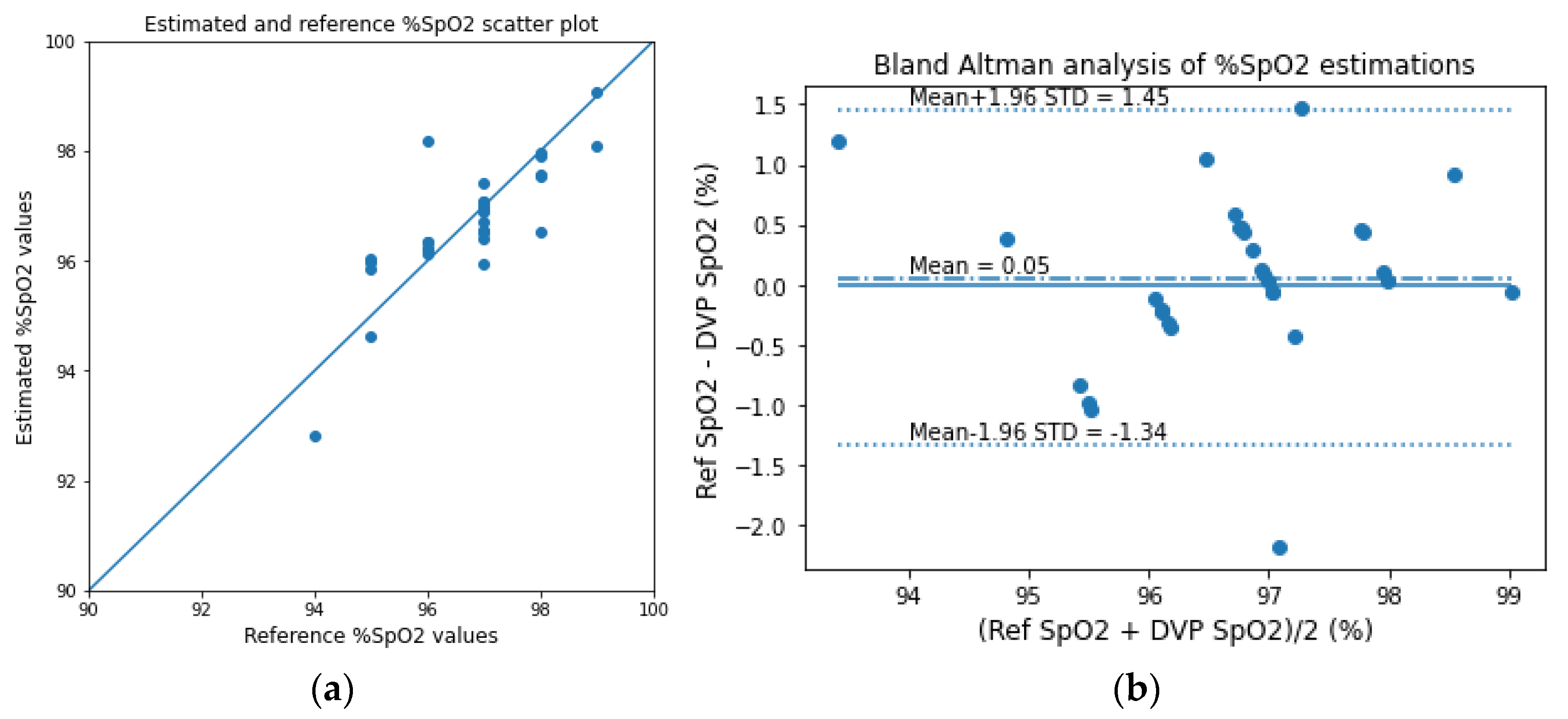
3.3.2. Fingertip: Reflection-Type
3.3.3. Wrist: One PD and Multiple Wavelength LEDs
3.4. Results Comparison
4. Discussion
5. Conclusions
Author Contributions
Funding
Institutional Review Board Statement
Informed Consent Statement
Data Availability Statement
Conflicts of Interest
Appendix A
Derivation Process
Appendix B
Features

| Serial | Feature Description | Feature |
|---|---|---|
| 1 | Systolic peak, | |
| 2 | Diastolic peak, | |
| 3 | Dicrotic notch, | |
| 4 | Pulse interval, | |
| 5 | Augmentation index | |
| 6 | Relative augmentation index | |
| 7 | ||
| 8 | ||
| 9 | Systolic peak time, | |
| 10 | Dicrotic notch time, | |
| 11 | Diastolic peak time, | |
| 12 | Time between dicrotic notch and diastolic peak, | |
| 13 | Time between half systolic peak points, | |
| 14 | Inflection point area ratio, | |
| 15 | Systolic peak rising slope | |
| 16 | Diastolic peak falling slope | |
| 17 | ||
| 18 | ||
| 19 | ||
| 20 | ||
| 21 | ||
| 22 | ||
| 23 | ||
| 24 | ||
| 25 | ||
| 26 | ||
| 27 | ||
| 28 | ||
| 29 | ||
| 30 | ||
| 31 | ||
| 32 | ||
| 33 | ||
| 34 | ||
| 35 | ||
| 36 | ||
| 37 | ||
| 38 | ||
| 39 | ||
| 40 | Fundamental component frequency | |
| 41 | Fundamental component magnitude | |
| 42 | 2nd harmonic frequency | |
| 43 | 2nd harmonic magnitude | |
| 44 | 3rd harmonic frequency | |
| 45 | 3rd harmonic magnitude |

References
- Chen, C.; Xie, Q.; Yang, D.; Xiao, H.; Fu, Y.; Tan, Y.; Yao, S. Recent advances in electrochemical glucose biosensors: A review. RSC Adv. 2013, 3, 4473–4491. [Google Scholar] [CrossRef]
- Bandodkar, A.J.; Wang, J. Non-invasive wearable electrochemical sensors: A review. Trends Biotechnol. 2014, 32, 363–371. [Google Scholar] [CrossRef] [PubMed]
- Sharma, S.; Huang, Z.; Rogers, M.; Boutelle, M.; Cass, A.E.G. Evaluation of a minimally invasive glucose biosensor for continuous tissue monitoring. Anal. Bioanal. Chem. 2016, 408, 8427–8435. [Google Scholar] [CrossRef] [Green Version]
- Haque, C.A.; Hossain, S.; Kwon, T.-H.; Kim, K.-D. Noninvasive In Vivo Estimation of Blood-Glucose Concentration by Monte Carlo Simulation. Sensors 2021, 21, 4918. [Google Scholar] [CrossRef]
- Little, R.R.; Roberts, W.L. A Review of Variant Hemoglobins Interfering with Hemoglobin A1c Measurement. J. Diabetes Sci. Technol. Online 2009, 3, 446–451. [Google Scholar] [CrossRef] [Green Version]
- Mandal, S.; Manasreh, M.O. An In-Vitro Optical Sensor Designed to Estimate Glycated Hemoglobin Levels. Sensors 2018, 18, 1084. [Google Scholar] [CrossRef] [PubMed] [Green Version]
- Martín-Mateos, P.; Dornuf, F.; Duarte, B.; Hils, B.; Moreno-Oyervides, A.; Bonilla-Manrique, O.E.; Larcher, F.; Krozer, V.; Acedo, P. In-vivo, non-invasive detection of hyperglycemic states in animal models using mm-wave spectroscopy. Sci. Rep. 2016, 6, 34035. [Google Scholar] [CrossRef] [Green Version]
- Usman, S.; Bani, N.A.; Mad Kaidi, H.; Mohd Aris, S.A.; Zura, A.; Jalil, S.; Muhtazaruddin, M.N. Second Derivative and Contour Analysis of PPG for Diabetic Patients. In Proceedings of the 2018 IEEE-EMBS Conference on Biomedical Engineering and Sciences (IECBES), Kuala Lumpur, Malaysia, 3–6 December 2018. [Google Scholar] [CrossRef]
- Saraoğlu, H.M.; Selvi, A.O. Determination of glucose and Hba1c values in blood from human breath by using Radial Basis Function Neural Network via electronic nose. In Proceedings of the 2014 18th National Biomedical Engineering Meeting, Istanbul, Turkey, 16–17 October 2014. [Google Scholar] [CrossRef]
- Hossain, S.; Gupta, S.S.; Kwon, T.-H.; Kim, K.-D. Derivation and Validation of Gray-Box Models to Estimate Noninvasive In-vivo Percentage Glycated Hemoglobin Using Digital Volume Pulse Waveform. Sci. Rep. 2021, 11, 12169. [Google Scholar] [CrossRef]
- Hossain, M.S.; Kim, K.-D. Noninvasive Estimation of Glycated Hemoglobin In-Vivo Based on Photon Diffusion Theory and Genetic Symbolic Regression Models. IEEE Trans. Biomed. Eng. 2021, 69, 2053–2064. [Google Scholar] [CrossRef]
- Wang, B.; Matcuk, G.; Barbič, J. Hand MRI Dataset; University of Southern California: Los Angeles, CA, USA, 2020. [Google Scholar]
- Meglinski, I.V.; Matcher, S.J. Quantitative assessment of skin layers absorption and skin reflectance spectra simulation in the visible and near-infrared spectral regions. Physiol. Meas. 2002, 23, 741–753. [Google Scholar] [CrossRef]
- Jacques, S.L. Origins of Tissue Optical Properties in the UVA, Visible, and NIR Regions. In Advances in Optical Imaging and Photon Migration; Optica Publishing Group: Washington, DC, USA, 1996; Volume 2, pp. 364–371. [Google Scholar]
- Chatterjee, S.; Kyriacou, P.A. Monte Carlo Analysis of Optical Interactions in Reflectance and Transmittance Finger Photoplethysmography. Sensors 2019, 19, 789. [Google Scholar] [CrossRef] [PubMed] [Green Version]
- Wisotzky, E.L.; Uecker, F.C.; Dommerich, S.; Hilsmann, A.; Eisert, P.; Arens, P. Determination of optical properties of human tissues obtained from parotidectomy in the spectral range of 250 to 800 nm. J. Biomed. Opt. 2019, 24, 125001. [Google Scholar] [CrossRef] [PubMed]
- Genina, E.A.; Bashkatov, A.N.; Tuchin, V.V. Optical Clearing of Cranial Bone. Adv. Opt. Technol. 2008, 2008, e267867. [Google Scholar] [CrossRef] [Green Version]
- Jacques, S.L. Optical properties of biological tissues: A review. Phys. Med. Biol. 2013, 58, R37–R61. [Google Scholar] [CrossRef]
- Prahl, S.A. Tabulated Molar Extinction Coefficient for Hemoglobin in Water. 1998. Available online: https://omlc.org/spectra/hemoglobin/summary.html (accessed on 29 December 2022).
- Hossain, S.; Kwon, T.-H.; Kim, K.-D. Estimation of Molar Absorption Coefficients of HbA1c in Near UV-Vis-SW NIR Light Spectrum. Korean Inst. Commun. Inf. Sci. 2021, 46, 1030–1039. [Google Scholar] [CrossRef]
- Friebel, M.; Roggan, A.; Müller, G.; Meinke, M. Determination of optical properties of human blood in the spectral range 250 to 1100 nm using Monte Carlo simulations with hematocrit-dependent effective scattering phase functions. J. Biomed. Opt. 2006, 11, 34021. [Google Scholar] [CrossRef] [PubMed]
- Schulz, B.; Chan, D.; Bäckström, J.; Rübhausen, M.; Wittern, K.P.; Wessel, S.; Wepf, R.; Williams, S. Hydration dynamics of human fingernails: An ellipsometric study. Phys. Rev. E Stat. Nonlinear Soft Matter Phys. 2002, 65 Pt 1, 061913. [Google Scholar] [CrossRef]
- Steenbergen, W.; Kolkman, R.; de Mul, F. Light-scattering properties of undiluted human blood subjected to simple shear. J. Opt. Soc. Am. A 1999, 16, 2959–2967. [Google Scholar] [CrossRef] [PubMed]
- Elblbesy, M.A.; Elblbesy, M.A. The refractive index of human blood measured at the visible spectral region by single-fiber reflectance spectroscopy. AIMS Biophys. 2021, 8, 57–65. [Google Scholar] [CrossRef]
- Bashkatov, A.N.; Genina, E.A.; Tuchin, V.V. Optical properties of skin, subcutaneous, and muscle tissues: A review. J. Innov. Opt. Health Sci. 2011, 4, 9–38. [Google Scholar] [CrossRef]
- Slapničar, G.; Mlakar, N.; Luštrek, M. Blood Pressure Estimation from Photoplethysmogram Using a Spectro-Temporal Deep Neural Network. Sensors 2019, 19, 3420. [Google Scholar] [CrossRef] [PubMed] [Green Version]
- Zhang, X.; Lyu, Y.; Qu, T.; Qiu, P.; Luo, X.; Zhang, J.; Fan, S.; Shi, Y. Photoplethysmogram-based Cognitive Load Assessment Using Multi-Feature Fusion Model. ACM Trans. Appl. Percept. 2019, 16, 1–17. [Google Scholar] [CrossRef]


| Skin Sublayer Name | Layer Thickness [mm] | ||||
|---|---|---|---|---|---|
| Stratum corneum | 0 | 0 | 0.05 | 0 | 0.02 |
| Epidermis | 0 | 0 | 0.2 | 0.1 | 0.25 |
| Papillary dermis | 0.02 | 0.02 | 0.5 | 0 | 0.1 |
| Upper blood net dermis | 0.15 | 0.15 | 0.6 | 0 | 0.08 |
| Reticular dermis | 0.02 | 0.02 | 0.7 | 0 | 0.2 |
| Deep blood net dermis | 0.05 | 0.05 | 0.05 | 0 | 0.3 |
| Material | Absorption Coefficient | Scattering Coefficient | Anisotropy Factor | Refractive Index | ||||
|---|---|---|---|---|---|---|---|---|
| 465 nm | 525 nm | 615 nm | 465 nm | 525 nm | 615 nm | |||
| Oxyhemoglobin | 8.94 | 7.18 | 0.27 | - | - | - | ||
| Deoxyhemoglobin | 4.35 | 8.18 | 1.76 | - | - | - | ||
| Glycated hemoglobin | 127.68 | 105.85 | 39.66 | - | - | - | ||
| Whole blood | - | 84.61 | 59.17 | 53.00 | 0.995 [23] | 1.354 [24] | ||
| Melanin | 88.66 | 58.12 | 33.51 | - | - | - | ||
| Skin baseline | 0.163 | 0.110 | 0.066 | - | - | - | ||
| Muscle | 0.88 | 1.17 | 0.22 | 2.41 | 1.71 | 1.09 | 0.5 [15] | 1.37 [25] |
| Fat | 0.005 | 0.001 | 0.0004 | 6.47 | 5.96 | 5.35 | 0.75 [13] | 1.44 [25] |
| Bone | 0.118 | 0.118 | 0.068 | 53.40 | 44.68 | 35.41 | 0.92 [15] | 1.37 [17] |
| Nail | 0.012 | 21 | 0.90 [22] | 1.51 [22] | ||||
| Dataset | HbA1c (%) | SpO2 (%) | Age (Mean ± SD) | BMI (Mean ± SD) | ||||
|---|---|---|---|---|---|---|---|---|
| Min | Max | Mean ± SD | Min | Max | Mean ± SD | |||
| Fingertip | 4.9 | 9.1 | 6.08 ± 0.99 | 94 | 99 | 96.74 ± 1.16 | 34.6 ± 13.01 | 27.87 ± 4.05 |
| Wrist | 4.9 | 8.4 | 6.01 ± 0.90 | 95 | 98 | 96.68 ± 0.80 | 42.67 ± 15.11 | 25.60 ± 4.15 |
| MSE | ME | MAD | RMSE | Pearson’s r |
|---|---|---|---|---|
| 0.13 | −0.003 | 0.19 | 0.36 | 0.94 |
| MSE | ME | MAD | RMSE | RCF |
|---|---|---|---|---|
| 0.39 | 0.10 | 0.46 | 0.62 | 0.9953 |
| MSE | ME | MAD | RMSE | Pearson’s r |
|---|---|---|---|---|
| 0.06 | 0.01 | 0.16 | 0.25 | 0.96 |
| MSE | ME | MAD | RMSE | RCF |
|---|---|---|---|---|
| 0.51 | 0.05 | 0.51 | 0.71 | 0.9948 |
| MSE | ME | MAD | RMSE | Pearson’s r |
|---|---|---|---|---|
| 0.05 | 0.01 | 0.13 | 0.21 | 0.97 |
| MSE | ME | MAD | RMSE | RCF |
|---|---|---|---|---|
| 0.06 | −0.03 | 0.19 | 0.25 | 0.9981 |
| Method | HbA1c Pearson’s r | SpO2 RCF |
|---|---|---|
| Beer–Lambert fingertip blood-vessel model [10] | 0.90 | 0.988 |
| Beer–Lambert fingertip whole-finger model [10] | 0.95 | 0.986 |
| Photon diffusion fingertip reflection model [26] | 0.91 | 0.988 |
| Photon diffusion fingertip transmission model [26] | 0.89 | 0.987 |
| Proposed Monte Carlo fingertip reflection model | 0.96 | 0.995 |
| Proposed Monte Carlo fingertip transmission model | 0.94 | 0.995 |
Disclaimer/Publisher’s Note: The statements, opinions and data contained in all publications are solely those of the individual author(s) and contributor(s) and not of MDPI and/or the editor(s). MDPI and/or the editor(s) disclaim responsibility for any injury to people or property resulting from any ideas, methods, instructions or products referred to in the content. |
© 2023 by the authors. Licensee MDPI, Basel, Switzerland. This article is an open access article distributed under the terms and conditions of the Creative Commons Attribution (CC BY) license (https://creativecommons.org/licenses/by/4.0/).
Share and Cite
Hossain, S.; Kim, K.-D. Non-Invasive In Vivo Estimation of HbA1c Using Monte Carlo Photon Propagation Simulation: Application of Tissue-Segmented 3D MRI Stacks of the Fingertip and Wrist for Wearable Systems. Sensors 2023, 23, 540. https://doi.org/10.3390/s23010540
Hossain S, Kim K-D. Non-Invasive In Vivo Estimation of HbA1c Using Monte Carlo Photon Propagation Simulation: Application of Tissue-Segmented 3D MRI Stacks of the Fingertip and Wrist for Wearable Systems. Sensors. 2023; 23(1):540. https://doi.org/10.3390/s23010540
Chicago/Turabian StyleHossain, Shifat, and Ki-Doo Kim. 2023. "Non-Invasive In Vivo Estimation of HbA1c Using Monte Carlo Photon Propagation Simulation: Application of Tissue-Segmented 3D MRI Stacks of the Fingertip and Wrist for Wearable Systems" Sensors 23, no. 1: 540. https://doi.org/10.3390/s23010540