
A Novel Analytical Modeling Approach for Quality Propagation of Transient Analysis of Serial Production Systems


Abstract
:1. Introduction
2. Problem Formulation and Modeling
2.1. Descriptive Models
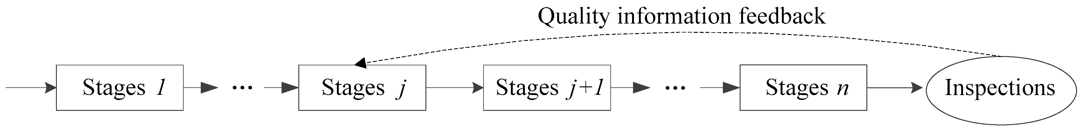
- The multistage production system is composed of stages with the inspection station in the final stage.
- The slots of the time axis are equal to the machine cycle time. Consider the working times of the production systems while the machine breakdown is not under consideration.
- The product quality processed in stage depends on the quality state of stage and the incoming product quality from upstream stage . Both quality corrections and quality degradations exist in production systems. The product could have better or worse quality after it is processed in a certain stage.
- With respect to the quality state of stage , denote stage as in the defective state or in the good state when stage produces a defective or good product in the time slot .
- With respect to the incoming product quality for stage , it relies on the upstream stage . Stage in the defective state or in the good state produces a defective or good product in the time slot , indicating a defective or a good incoming product for stage in the time slot , respectively.
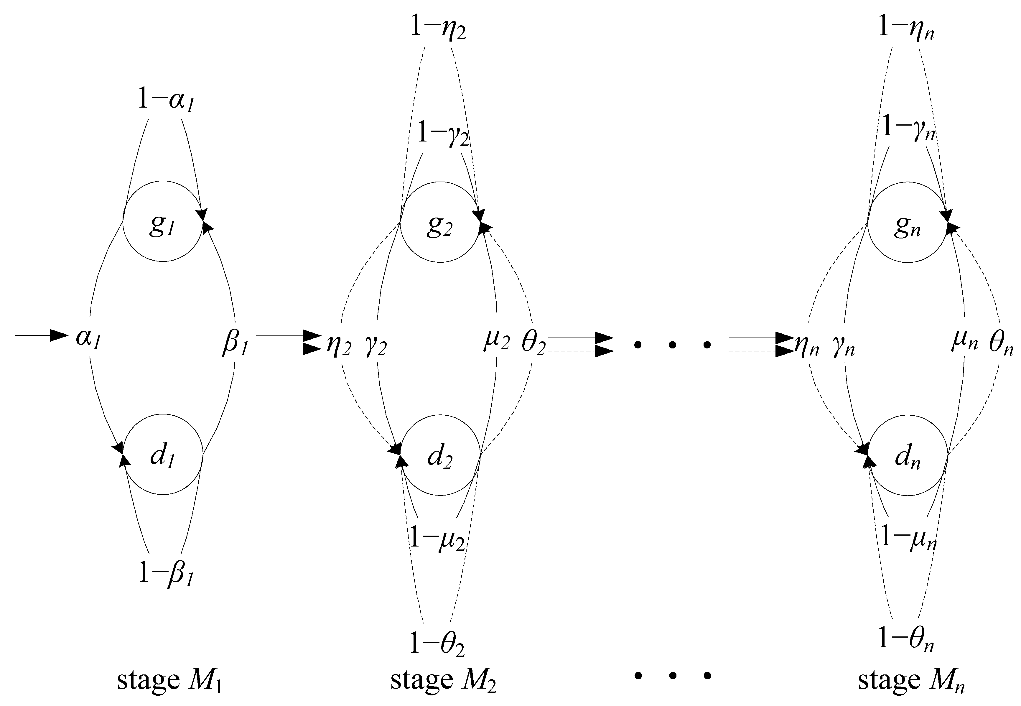
- When in the defective state , stage may transition into a good state with a probability or transition into a defective state with . When in a good state , stage may transition into a defective state with probability or transition into a good state with (see Figure 2).
2.2. Mathematical Models
3. Transient Quality Performance Evaluation of Two-Stage Production Systems
3.1. Two-Stage Production Systems with Constant Parameters
3.2. Two-Stage Production Systems with Time-Varying Parameters
4. Transient Quality Performance Evaluation of Multi-Stage Production Systems
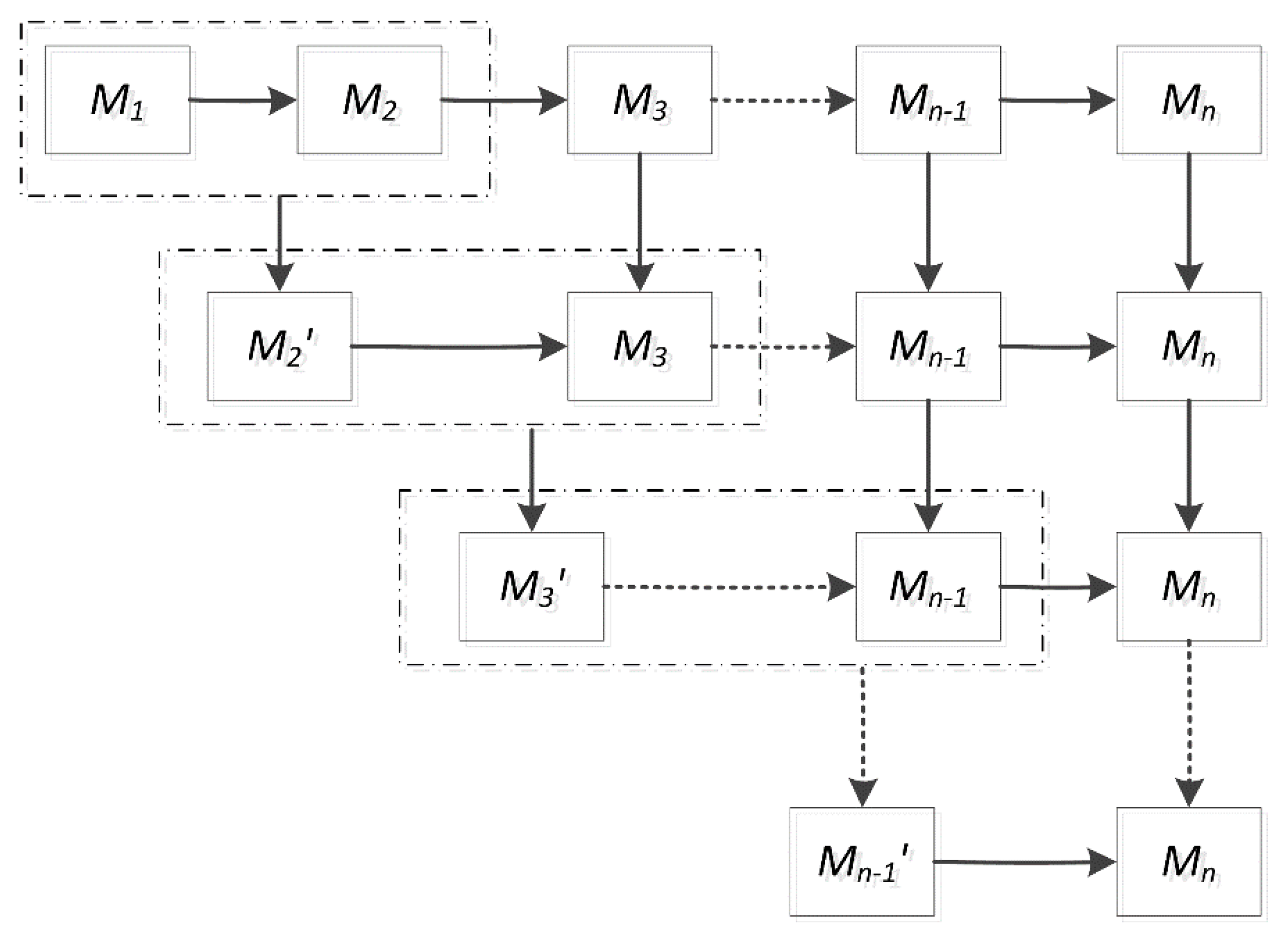
4.1. Aggregation-Based Approach for Multi-Stage Systems
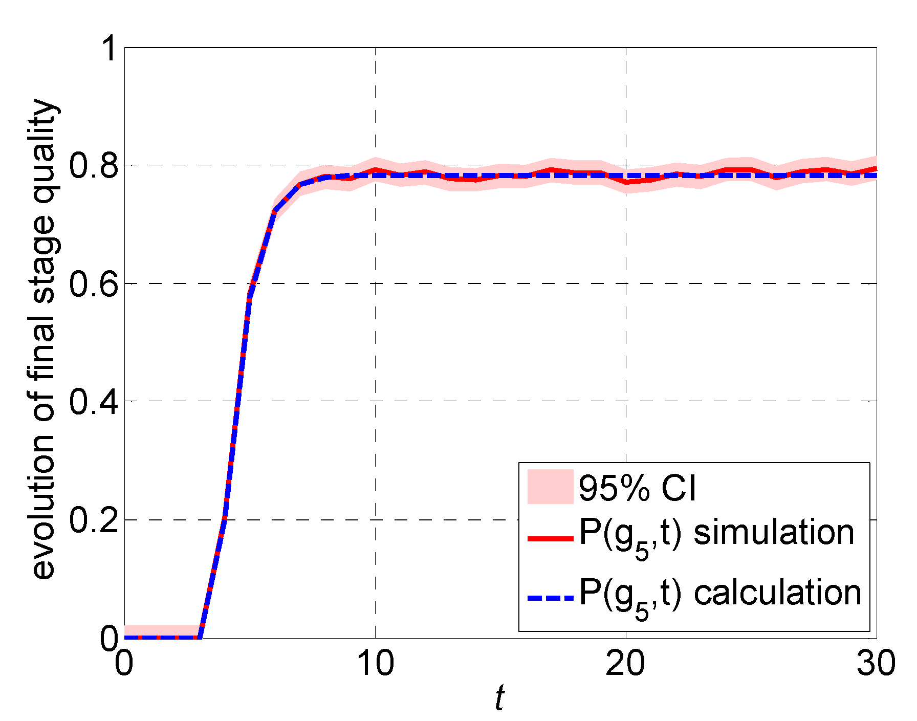
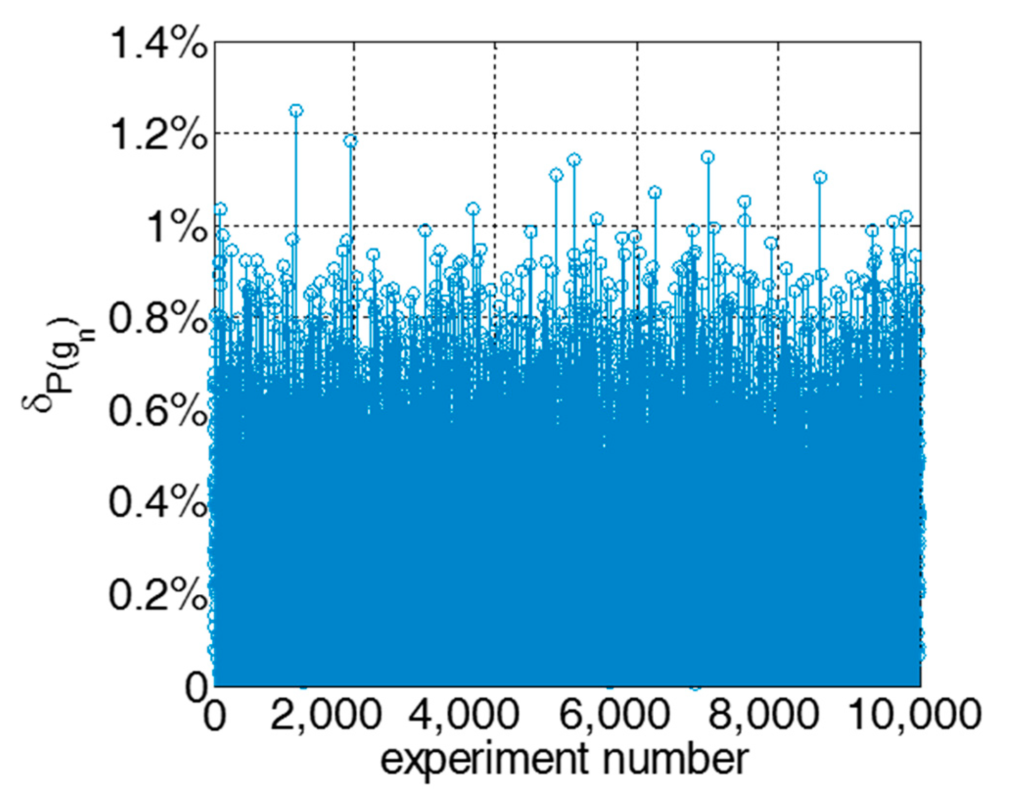
4.2. Model Accuracy Investigation
- Generate a setting of system parameters equiprobably and randomly among the following value sets.
- (1)
- The size–number of stages belong to .
- (2)
- The quality failure probability in case of an incoming product with good quality has a relatively small value, i.e., , .
- (3)
- The quality repair probability in case of an incoming product with good quality has a relatively large value, i.e., , .
- (4)
- The quality repair probability and failure probability in case of an incoming product with a defective quality, and .
- Conduct simulations for 200 time slots.
- Quality performance is unknown. Since the simulated performance measure is unbiased, the performance measure in the simulation is utilized for reflecting .
- Calculate the average value for performance measure during last 100 time slots. Moreover, the average is denoted as the simulated value of the steady-state quality.
5. Analysis of the System Theoretic Properties
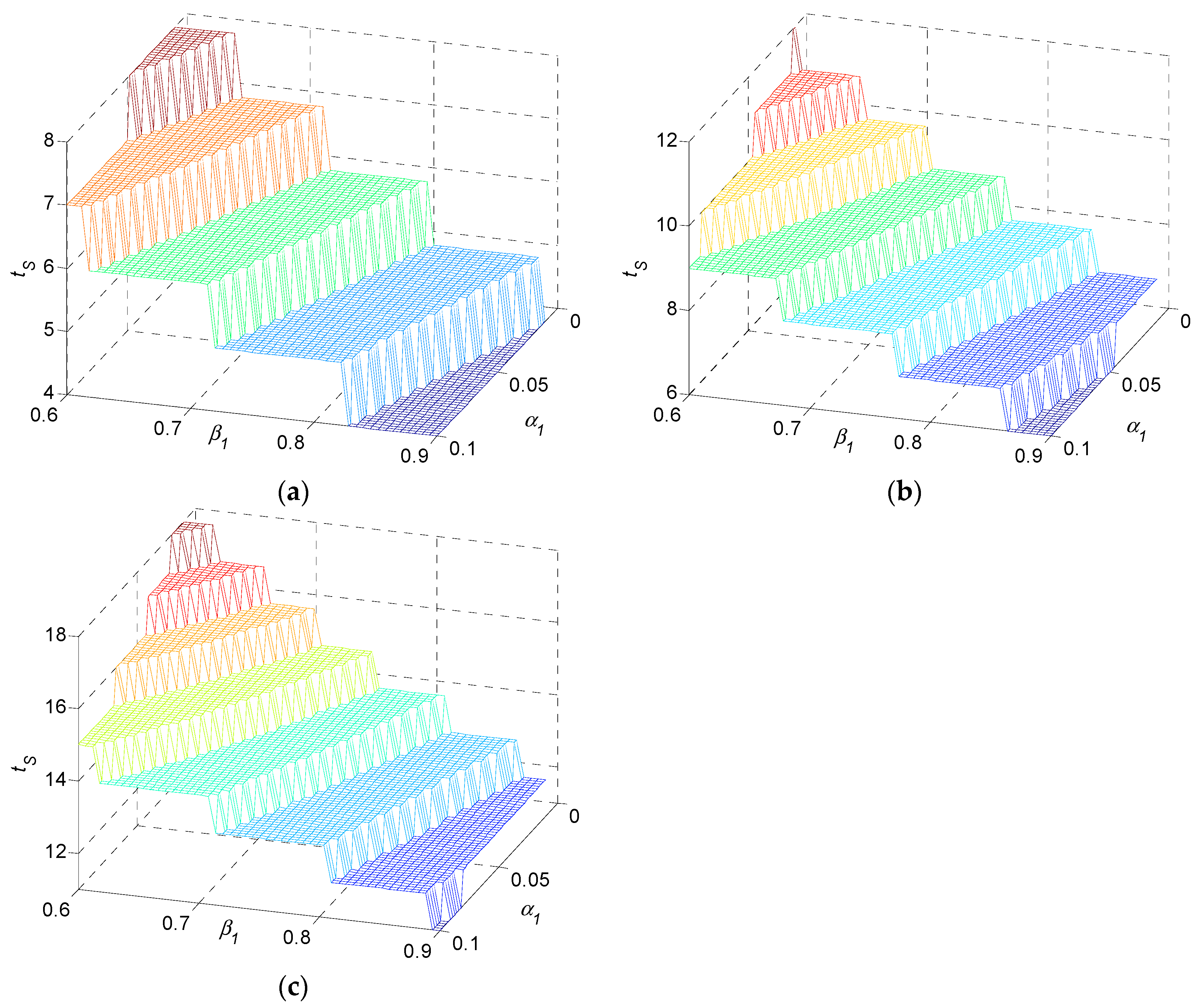
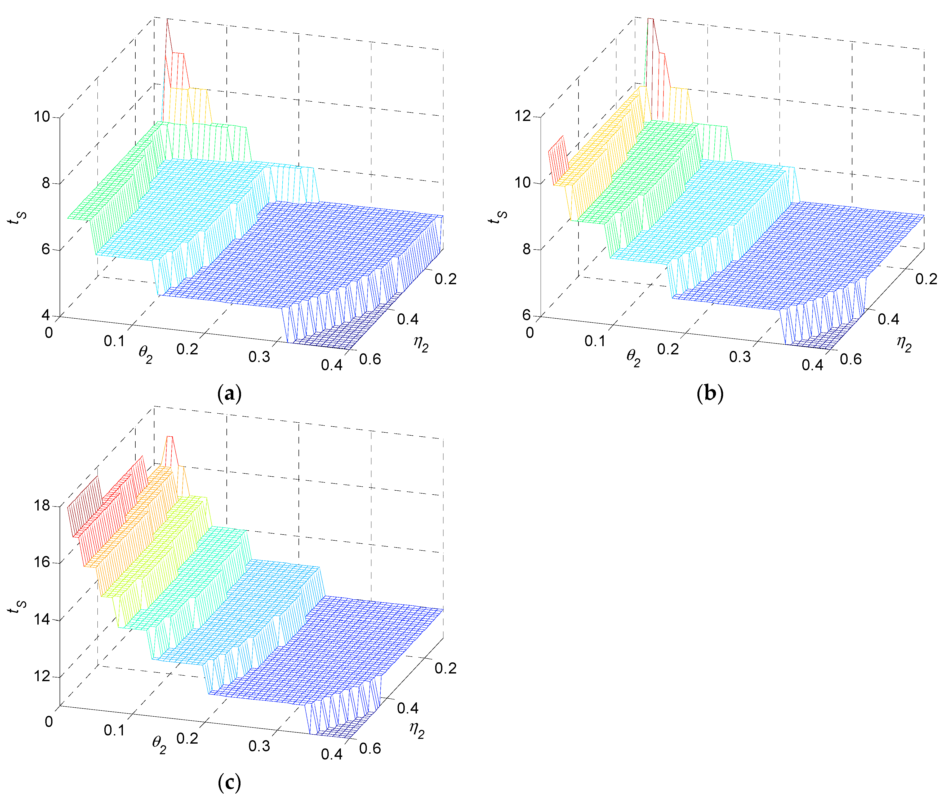
5.1. Analysis of Settling Time
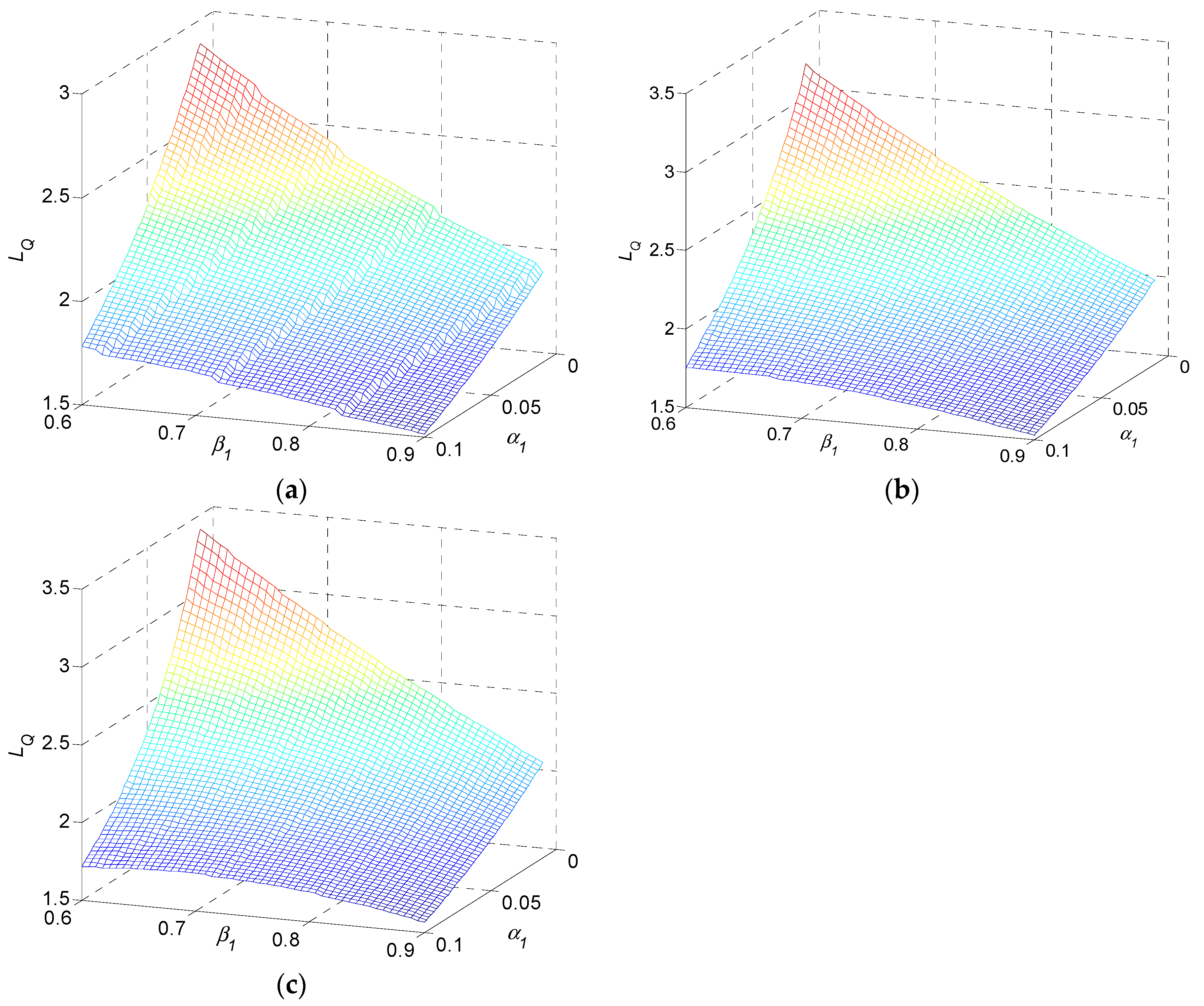
5.2. Analysis of Quality Loss
5.3. Steady-State Quality and Continuous Improvement Analysis
5.4. Bottleneck Analysis
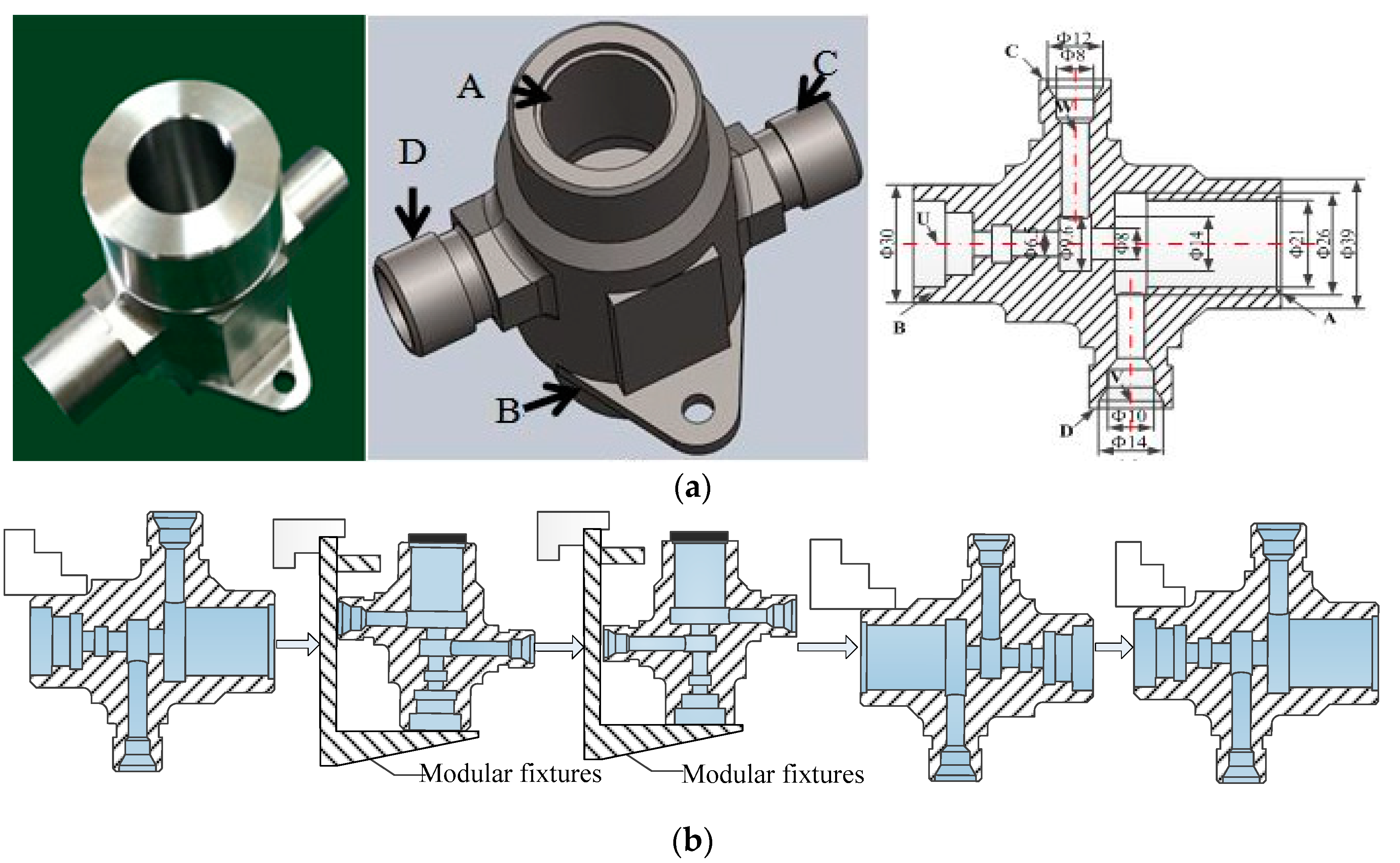
6. Case Study
6.1. Experimental Setup
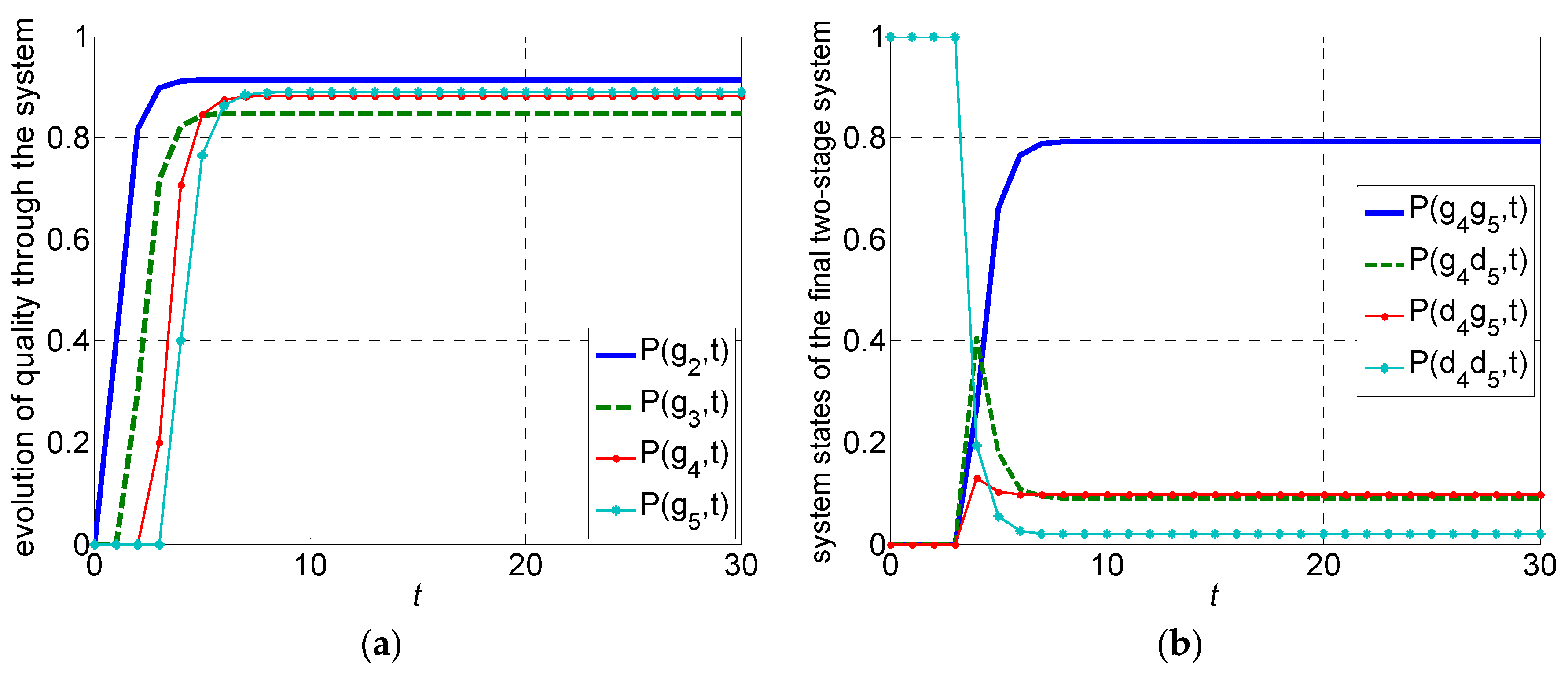
- (1)
- Last product after manufactured in is good, and product is good.
- (2)
- Last product after manufactured in is good, and product is defective.
- (3)
- Last product after manufactured in is defective, and product is good.
- (4)
- Last product after manufactured in is defective, and product is defective.
6.2. Modeling of Quality Performance
6.3. Structural Property Analysis and Quality Improvement
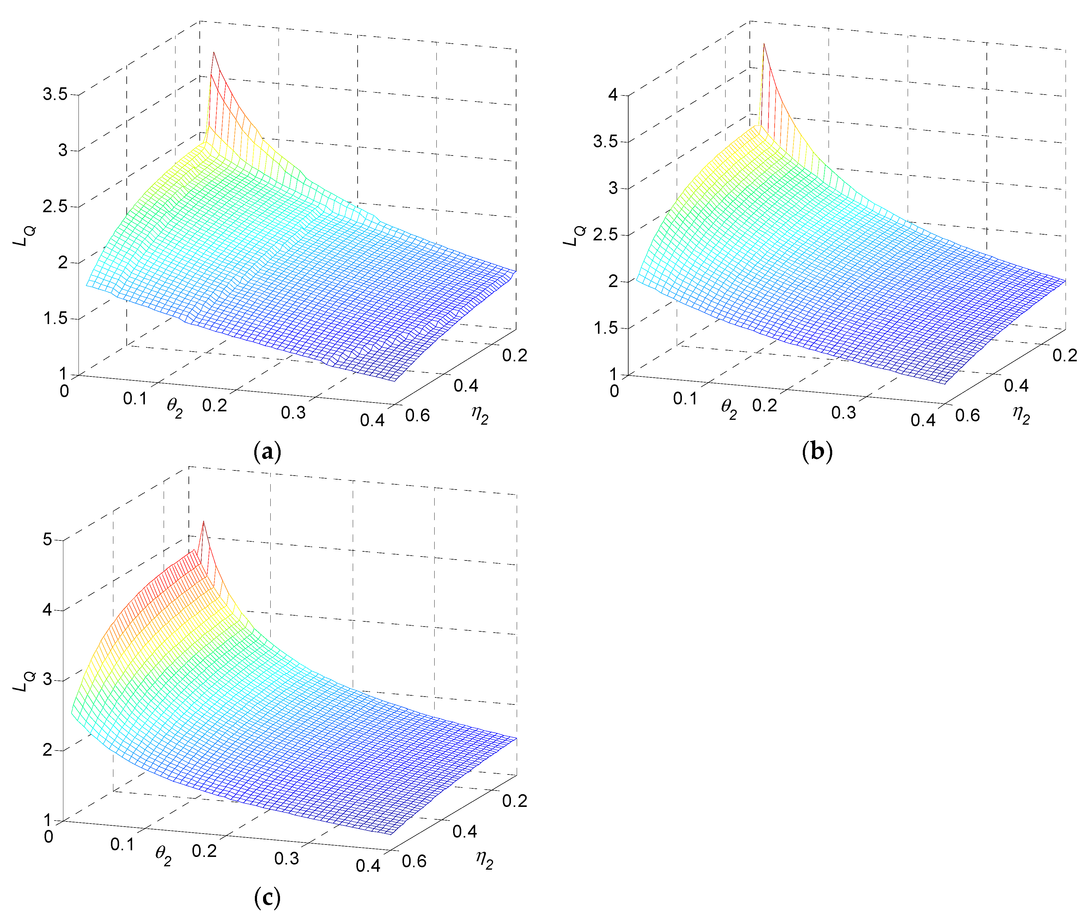
- (1)
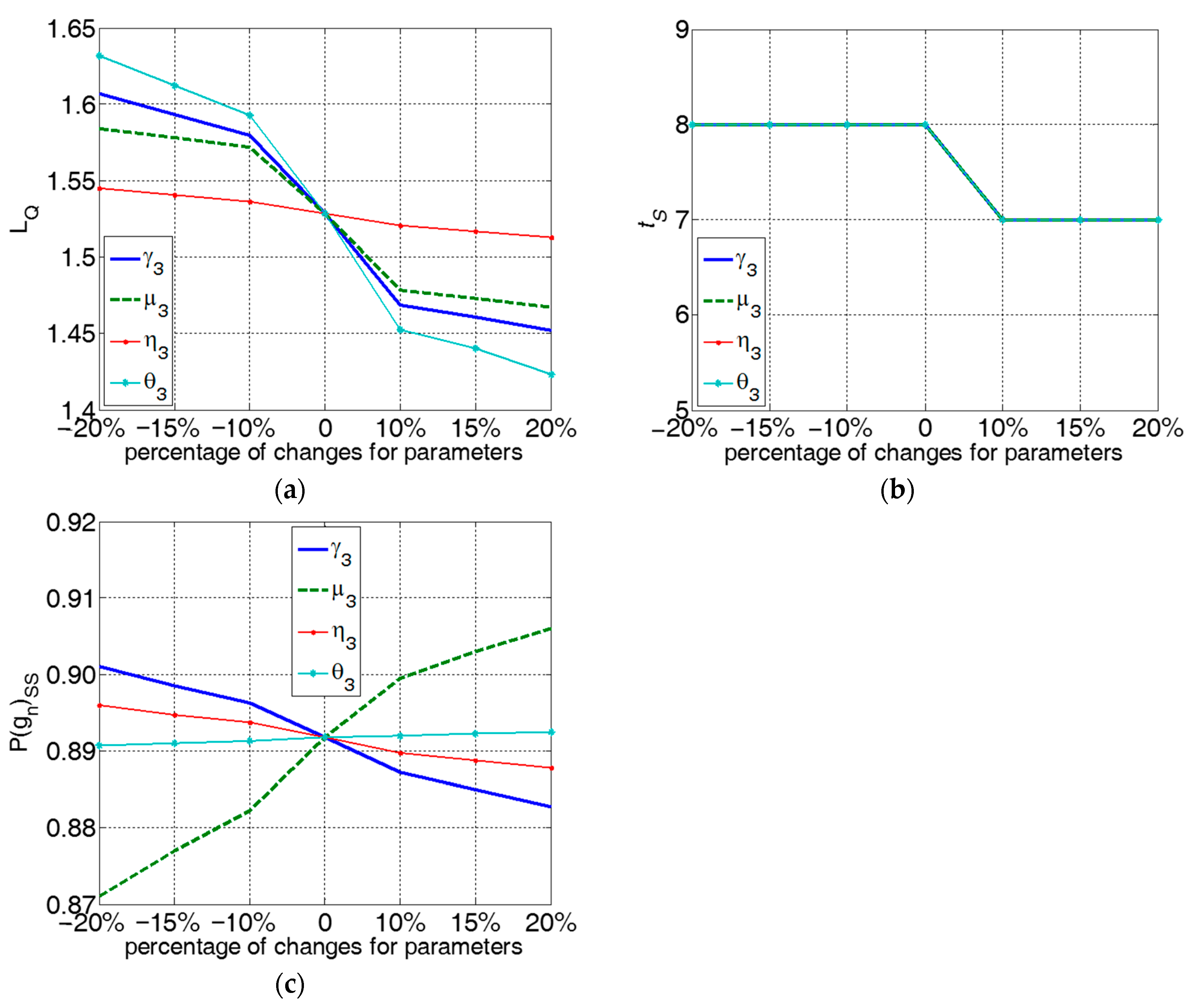
- From Figure 14a, the monotonic property for quality loss is in accordance with numerical results 3–4. Quality loss is decreased when system parameters of OP30 increase. According to the sensitivity analysis in the quality bottleneck stage, parameters QBN-, QBN-, QBN-, QBN- form the QBN set for OP30 with values {0.3900, 0.3285, 0.0510, 0.4947}. QBN- is denoted as the P-QBN. Quality loss in OP30 is most sensitive regarding quality repair probability in case of a defective incoming product . Proper changes of will bring the largest reduction to quality loss and prevent OP30 from being the quality bottleneck stage.
- (2)
- From Figure 14b, monotonic property for settling time is consistent with numerical results 1–2. The settling time will be reduced when the system parameter increases. As shown in Figure 6 and Figure 7, since settling time is eight or seven time slots in the range sets of transition probability given above, the four curves regarding parameters overlap in this case study.
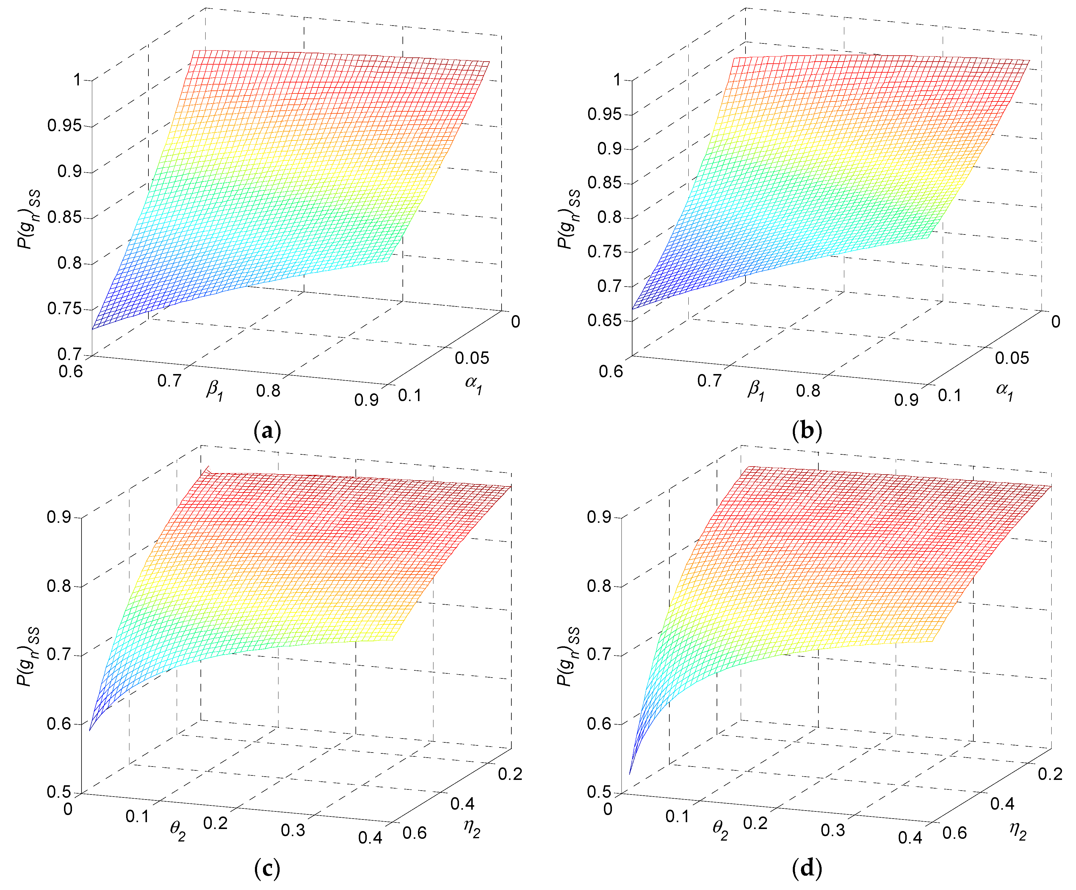
- (3)
- From Figure 14c, monotonic property for the steady-state quality is consistent with numerical result 5. Steady-state quality will improve when or increases, and when or decreases. In the sensitivity analysis, is the most sensitive parameter. Improving quality repair probability in case of a good incoming product achieves a better steady-state quality.The most sensitive parameter of steady-state quality is viewed as the quality bottleneck parameter in a steady-state phase. Correspondingly, the QBN set and P-QBN are viewed as quality bottleneck parameters in the transient phase. In some cases, the transient bottleneck parameter and steady-state bottleneck parameter are just the same parameter. However, in other cases, the two parameters may be different. As shown in the case study, they are and respectively.
- (4)
- When transient and steady-state quality bottleneck parameters fall in the same parameter, there is a desire to improve this particular parameter to facilitate quality performance in both the transient and steady-state regime. When they fall in different parameters, we can attempt to seek a balance between transients and the steady-state. Firstly, if production time horizon is relatively long, or when designing long-term production systems, we should focus on the steady-state quality bottleneck parameter since transients can be neglected compared with the overall production; on the contrary, we may focus on the transient quality bottleneck parameter. Secondly, if the criterion of quality loss rate is high, focus on the transient bottleneck parameter to prioritize reduction in quality loss; contrarily, focus on the steady-state bottleneck parameter.
7. Conclusions
Author Contributions
Funding
Institutional Review Board Statement
Informed Consent Statement
Data Availability Statement
Conflicts of Interest
Notations
| Mi | ith stage of multi-stage production systems |
| Mi′ | the merged stage from the first i stages of multi-stage production systems |
| gi | Mi or Mi′ produces a good product |
| di | Mi or Mi′ produces a defective product |
| α1 | probability of M1 transiting from g1 to d1 |
| β1 | probability of M1 transiting from d1 to g1 |
| αi′ | probability of Mi′ transiting from gi to di |
| βi′ | probability of Mi′ transiting from di to gi |
| γi | in case of good coming product, probability of Mi transiting from state gi to di |
| μi | in case of good coming product, probability of Mi transiting from state di to gi |
| ηi | in case of defective coming product, probability of Mi transiting from state gi to di |
| θi | in case of defective coming product, probability of Mi transiting from state di to gi |
| gigi+1 | Mi or Mi′ produces good product, Mi+1 produces good product |
| gidi+1 | Mi or Mi′ produces good product, Mi+1 produces defective product |
| digi+1 | Mi or Mi′ produces defective product, Mi+1 produces good product |
| didi+1 | Mi or Mi′ produces defective product, Mi+1 produces defective product |
| Si(t) | state probability matrix with i stage at time slot t |
| Ci | state transition probability matrix with i stage |
| P(git) | probability of producing good product with i stage at time slot t |
| P(gi)ss | probability of producing good product with i stage in steady-state |
| ts | settling time for system quality to approach steady-state |
| LQ | quality loss during transients |
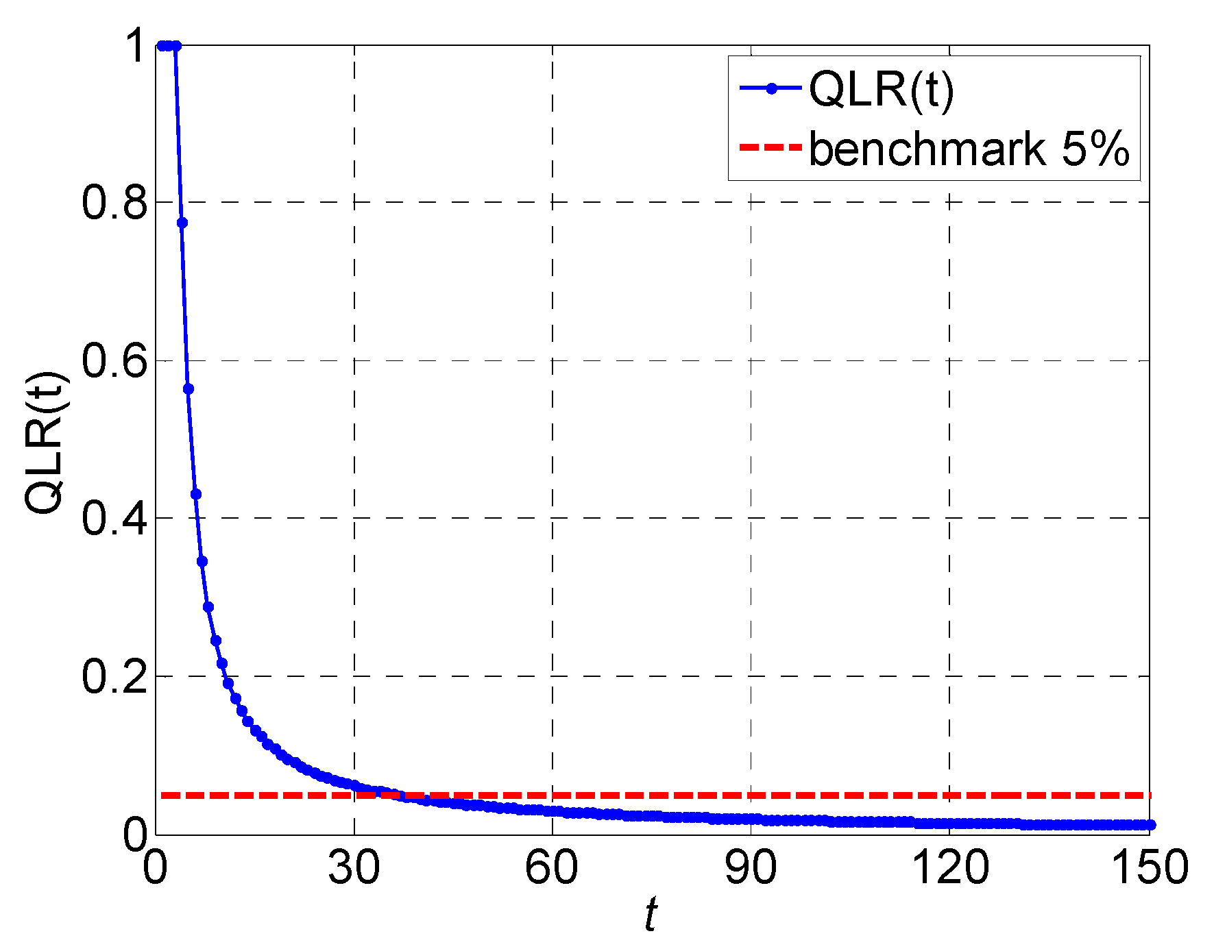
| QLR(t) | quality loss rate over t time slots |
| QBN– | quality bottleneck parameters |
References
- Jin, J.; Shi, J. State space modeling of sheet metal assembly for dimensional control. ASME Trans. J. Manuf. Sci. Eng. 1999, 121, 756–762. [Google Scholar] [CrossRef]
- Shi, J.; Zhou, S. Quality control and improvement for multistage systems: A survey. IIE Trans. 2009, 41, 744–753. [Google Scholar] [CrossRef]
- Du, S.; Yao, X.; Huang, D. Engineering model-based Bayesian monitoring of ramp-up phase of multistage manufacturing process. Int. J. Prod. Res. 2015, 53, 4594–4613. [Google Scholar] [CrossRef]
- Yang, F.; Jin, S.; Li, Z. A modification of DMVs based state space model of variation propagation for multistage machining processes. Assem. Autom. 2017, 37, 381–390. [Google Scholar] [CrossRef]
- Wang, K.; Li, G.; Du, S.; Xi, L.; Xia, T. State space modelling of variation propagation in multistage machining processes for variable stiffness structure workpieces. Int. J. Prod. Res. 2021, 59, 4033–4052. [Google Scholar] [CrossRef]
- Zhao, C.; Li, J.; Huang, N.; Horst, J.A. Flexible Serial Lines with Setups: Analysis, Improvement, and Application. IEEE Robot. Autom. Lett. 2016, 2, 120–127. [Google Scholar] [CrossRef]
- Du, S.; Xu, R.; Li, L. Modeling and analysis of multiproduct multistage manufacturing systems for quality improvement. IEEE Trans. Syst. Man Cybern. Syst. 2018, 48, 801–820. [Google Scholar] [CrossRef]
- Şahin, A.; Sayımlar, A.D.; Teksan, Z.M.; Albey, E. A Markovian Approach for Time Series Prediction for Quality Control. IFAC-Pap. Online 2019, 52, 1902–1907. [Google Scholar] [CrossRef]
- Goswami, M.; Kumar, G.; Ghadge, A. An integrated Bayesian–Markovian framework for ascertaining cost of executing quality improvement programs in manufacturing industry. Int. J. Qual. Reliab. Manag. 2019, 36, 1229–1242. [Google Scholar] [CrossRef]
- Guo, W.; Gu, X. Joint decision-making of production and maintenance in mixed model assembly systems with delayed differentiation configurations. Int. J. Prod. Res. 2020, 58, 4071–4085. [Google Scholar] [CrossRef]
- Yaghoubi, A.; Rahimi, S.; Soltani, R.; Akhavan Niaki, S.T. Availability analysis of a cooking oil production line. J. Optim. Ind. Eng. 2021, 14, 1–9. [Google Scholar]
- Ju, F.; Li, J.; Xiao, G.; Arinez, J.; Deng, W. Modeling, analysis, and improvement of integrated productivity and quality systems in battery manufacturing. IIE Trans. 2015, 47, 1313–1328. [Google Scholar] [CrossRef]
- Xu, W.; Cao, L. Optimal maintenance control of machine tools for energy efficient manufacturing. Int. J. Adv. Manuf. Technol. 2019, 104, 3303–3311. [Google Scholar] [CrossRef]
- Xiao, S.; Chen, Z.; Sarker, B. Integrated maintenance and production decision for k-out-of-n system equipment with attenuation of product quality. Int. J. Qual. Reliab. Manag. 2019, 36, 735–751. [Google Scholar] [CrossRef]
- Yaghoubi, A.; Niaki, S.T.A.; Rostamzadeh, H. A closed-form equation for steady-state availability of cold standby repairable k-out-of-n: G systems. Int. J. Qual. Reliab. Manag. 2020, 37, 145–155. [Google Scholar] [CrossRef]
- Zhang, Y.; Zhao, M.; Zhang, Y.; Pan, R.; Cai, J. Dynamic and steady-state performance analysis for multi-state repairable reconfigurable manufacturing systems with buffers. Eur. J. Oper. Res. 2020, 283, 491–510. [Google Scholar] [CrossRef]
- Gan, S.; Yousefi, N.; Coit, D.W. Optimal control-limit maintenance policy for a production system with multiple process states. Comput. Ind. Eng. 2021, 158, 107454. [Google Scholar] [CrossRef]
- Wu, C.H.; Zhou, F.Y.; Tsai, C.K.; Yu, C.J.; Dauzère-Pérès, S. A deep learning approach for the dynamic dispatching of unreliable machines in re-entrant production systems. Int. J. Prod. Res. 2020, 58, 2822–2840. [Google Scholar] [CrossRef]
- Lee, S.; Bain, P.A.; Musa, A.J.; Li, J. A Markov chain model for analysis of physician workflow in primary care clinics. Health Care Manag. Sci. 2021, 24, 72–91. [Google Scholar] [CrossRef]
- Liu, J.; Hu, Y.; Wu, B.; Wang, Y.; Xie, F. A hybrid generalized hidden Markov model-based condition monitoring approach for rolling bearings. Sensors 2017, 17, 1143. [Google Scholar] [CrossRef]
- Yu, Y.; Chen, Y. A measurement-based frame-level error model for evaluation of industrial wireless sensor networks. Sensors 2020, 20, 3978. [Google Scholar] [CrossRef]
- Gellert, A.; Sorostinean, R.; Pirvu, B. Robust assembly assistance using informed tree search with Markov chains. Sensors 2022, 22, 495. [Google Scholar] [CrossRef] [PubMed]
- Stavropoulos, P.; Papacharalampopoulos, A.; Stavridis, J.; Sampatakakis, K. A three-stage quality diagnosis platform for laser-based manufacturing processes. Int. J. Adv. Manuf. Technol. 2020, 110, 2991–3003. [Google Scholar] [CrossRef]
- Huang, J.; Meng, Y.; Liu, F.; Liu, C.; Li, H. Modeling and predicting inventory variation for multistage steel production processes based on a new spatio-temporal Markov model. Comput. Ind. Eng. 2022, 164, 107854. [Google Scholar] [CrossRef]
- Tang, Z.; Li, Y.; Chai, X.; Zhang, H.; Cao, S. Adaptive nonlinear model predictive control of NOx emissions under load constraints in power plant boilers. J. Chem. Eng. Jpn. 2020, 53, 36–44. [Google Scholar] [CrossRef] [Green Version]
- Park, K.; Li, J.; Feng, S. Scheduling policies in flexible bernoulli lines with dedicated finite buffers. J. Manuf. Syst. 2018, 48, 33–48. [Google Scholar] [CrossRef] [PubMed]
- Yang, F.; Liu, J. Simulation-based transfer function modeling for transient analysis of general queueing systems. Eur. J. Oper. Res. 2012, 223, 150–166. [Google Scholar] [CrossRef]
- Shaaban, S.; Hudson, S. Transient behaviour of unbalanced lines. Flex. Serv. Manuf. J. 2012, 24, 575–602. [Google Scholar] [CrossRef]
- Wang, M.; Huang, H.; Li, J. Transient Analysis of Multiproduct Bernoulli Serial Lines with Setups. IEEE Trans. Autom. Sci. Eng. 2021, 18, 135–150. [Google Scholar] [CrossRef]
- Wang, F.; Ju, F.; Kang, N. Transient analysis and real-time control of geometric serial lines with residence time constraints. IISE Trans. 2019, 51, 709–728. [Google Scholar] [CrossRef]
- Hou, Y.; Li, Y.; Ge, Y.; Zhang, J.; Jiang, S. Modeling of assembly systems with complex structures for throughput analysis during transients. Assem. Autom. 2019, 39, 262–271. [Google Scholar] [CrossRef]
- Gu, X.; Guo, W.; Jin, X. Performance evaluation for manufacturing systems under control-limit maintenance policy. J. Manuf. Syst. 2020, 55, 221–232. [Google Scholar] [CrossRef]
- Chen, W.; Liu, H.; Qi, E. Buffer allocation in asynchronous serial production systems with Bernoulli machines during transients. Int. J. Ind. Syst. Eng. 2021, 39, 176–204. [Google Scholar] [CrossRef]
- Sun, Y.; Zhu, T.; Zhang, L.; Denno, P. Parameter identification for Bernoulli serial production line model. IEEE Trans. Autom. Sci. Eng. 2021, 18, 2115–2127. [Google Scholar] [CrossRef]
- Zhou, B.; Lin, S. A novel analysis model for optimization performance of Bernoulli serial production systems considering rework processes. Proc. Inst. Mech. Eng. Part B J. Eng. Manuf. 2020, 234, 295–309. [Google Scholar] [CrossRef]
- Zhu, C.; Chang, Q.; Arinez, J. Data-enabled modeling and analysis of multistage manufacturing systems with quality rework loops. J. Manuf. Syst. 2020, 56, 573–584. [Google Scholar] [CrossRef]


Publisher’s Note: MDPI stays neutral with regard to jurisdictional claims in published maps and institutional affiliations. |
© 2022 by the authors. Licensee MDPI, Basel, Switzerland. This article is an open access article distributed under the terms and conditions of the Creative Commons Attribution (CC BY) license (https://creativecommons.org/licenses/by/4.0/).
Share and Cite
Liu, S.; Du, S.; Xi, L.; Shao, Y.; Huang, D. A Novel Analytical Modeling Approach for Quality Propagation of Transient Analysis of Serial Production Systems. Sensors 2022, 22, 2409. https://doi.org/10.3390/s22062409
Liu S, Du S, Xi L, Shao Y, Huang D. A Novel Analytical Modeling Approach for Quality Propagation of Transient Analysis of Serial Production Systems. Sensors. 2022; 22(6):2409. https://doi.org/10.3390/s22062409
Chicago/Turabian StyleLiu, Shihong, Shichang Du, Lifeng Xi, Yiping Shao, and Delin Huang. 2022. "A Novel Analytical Modeling Approach for Quality Propagation of Transient Analysis of Serial Production Systems" Sensors 22, no. 6: 2409. https://doi.org/10.3390/s22062409