
Imtidad: A Reference Architecture and a Case Study on Developing Distributed AI Services for Skin Disease Diagnosis over Cloud, Fog and Edge

 ,
,  , ,
, ,  and
and 
Abstract
:1. Introduction
- This is the first paper in which a reference architecture for distributed AI-as-a-service is proposed and implemented; a healthcare application (skin lesion diagnosis) is developed and studied in great detail, with a catalog containing several AI and Tiny AI services supported on multiple software, hardware, and networking platforms; and several use cases are evaluated using multiple benchmarks.
- The services are designed considering innovative use cases, such as a patient at home taking images of their skin lesion and performing the diagnosis by themselves with the help of a service or a travelling medical professional requesting a diagnosis from a fog device or cloud. The users of the services provided by this architecture can be patients, medical professionals, the patients’ family members, or any other stakeholder. Similarly, the services can be used by someone who has the disease diagnosis model, or the image, or both, since the resource (image or model) may be requested from other providers.
- The proposed work is highly novel and is expected to produce high impact due to the developed reference architecture; the service catalog offering a large number of services; the potential for the implementation of innovative use cases through the edge, fog, and cloud as well as their evaluation on many software, hardware, and networking platforms; and a detailed description of the architecture and case study.
- The existing works on distributed AI either focus on distributed AI methodologies [24,25] or distributed applications development [26,27,28], or application migration to fog and edge [29,30]. In contrast, this paper broadly aims to provide theoretical and applied contributions on decoupling application development from AI by using the distributed AI as a Service (DAIaaS) concept to coordinate, standardize, and streamline existing research on distributed AI and application migration to the edge. The decoupling of application development from AI is needed because it allows application, sensor, and IoT developers to focus on the various domain-specific details, relieve them from worries related to the how-to of distributed training and inference, and help systemize and mass-produce technologies for smarter environments. The Imtidad reference architecture and case study, given in this paper, outlines the whole process and roadmap of developing a service catalog using distributed AI as a Service, and, essentially, this provides a blueprint and procedure for decoupling applications and AI, enabling smart application development as a foundation for smarter societies. The approach allows development of unified interfaces to facilitate both independent and collaborative software development across different application domains. This is a continuation of our earlier research, where a DAIaaS concept was proposed and investigated using simulations [13].
2. Related Works
2.1. Distributed Artificial Intelligence (DAI) over Cloud, Fog, and Edge
2.1.1. Tiny AI and Edge: Research and Frameworks
2.1.2. Distributed AI in Healthcare
2.2. Skin Lesion Diagnosis
2.3. Research Gap
3. Imtidad Reference Architecture, Methodology, and Service Catalog
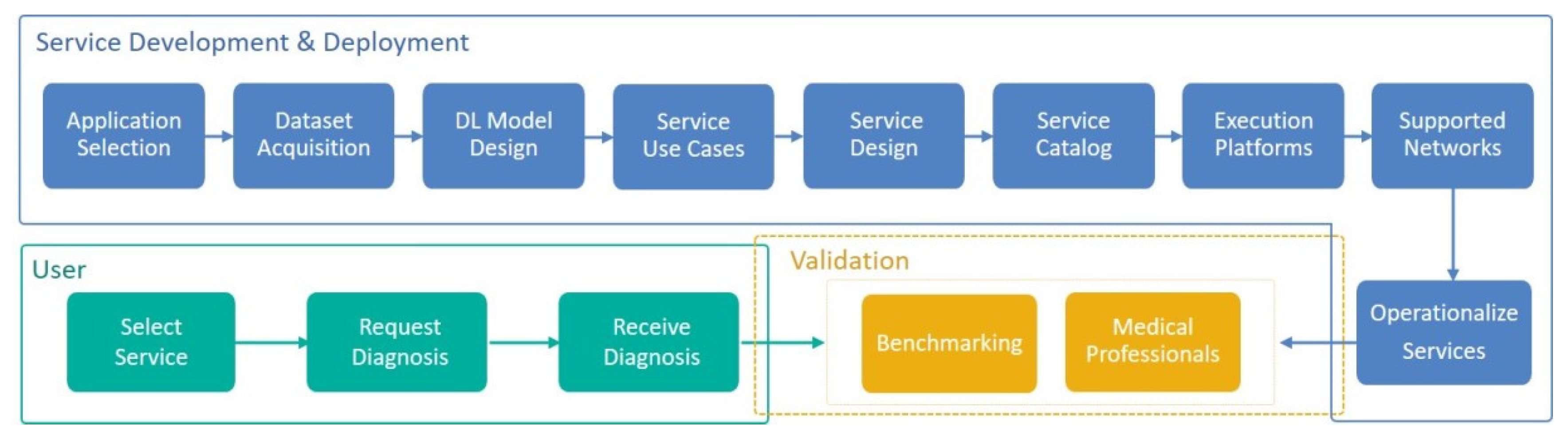
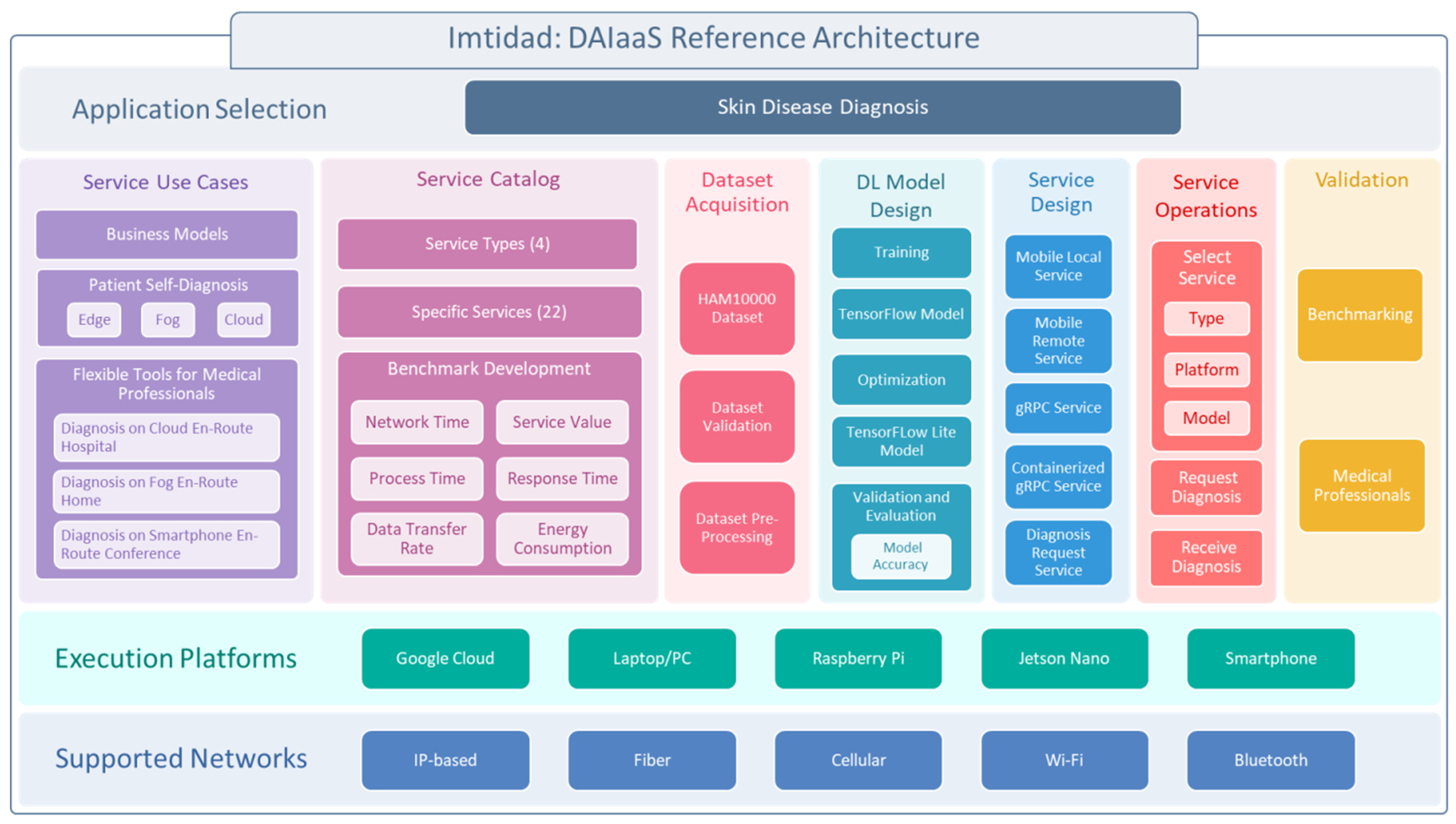
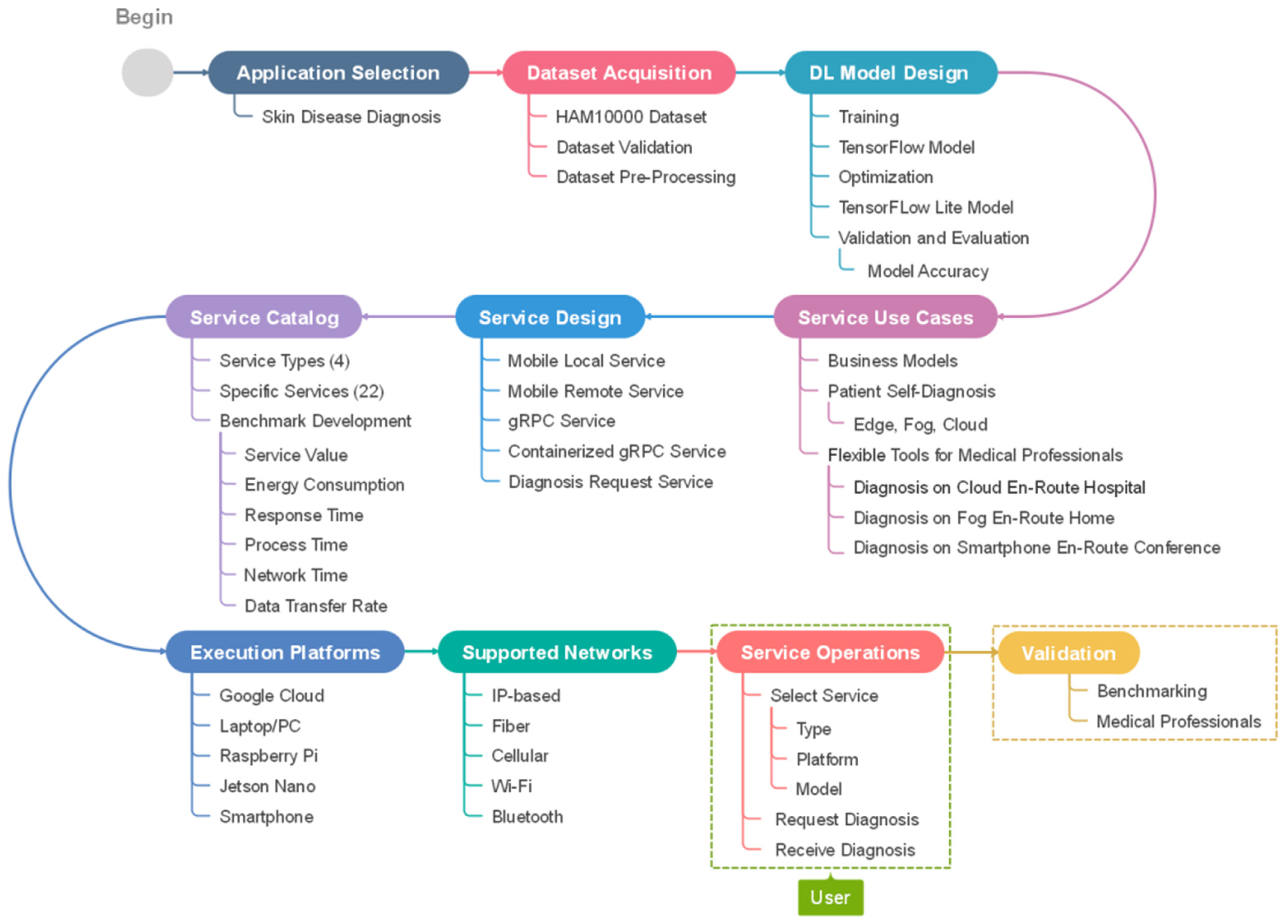
3.1. Reference Architecture and Methodology Overview
3.2. Service Use Cases
3.3. Service Catalog
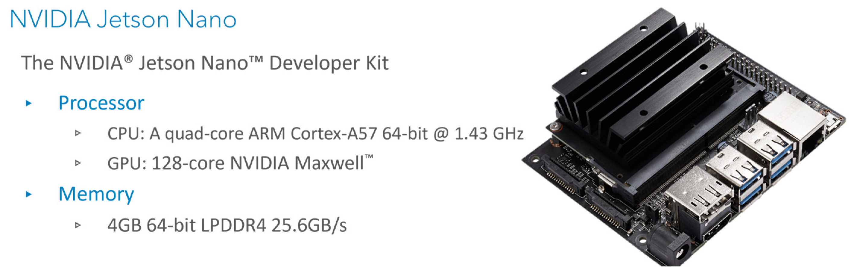
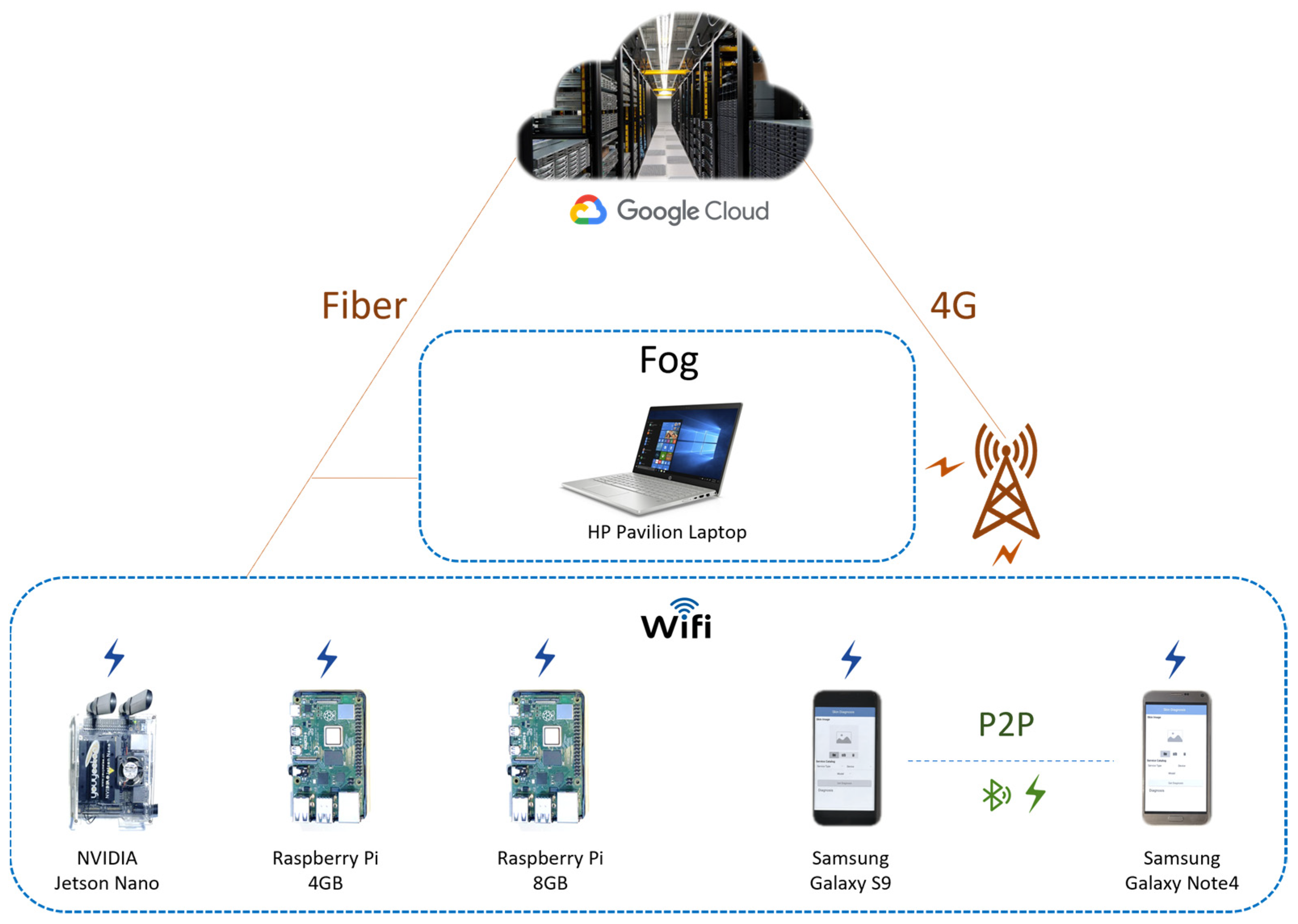
3.4. Devices and Hardware Platforms
3.5. Service Evaluation
4. System Architecture and Design (Skin Lesion Diagnosis Services)
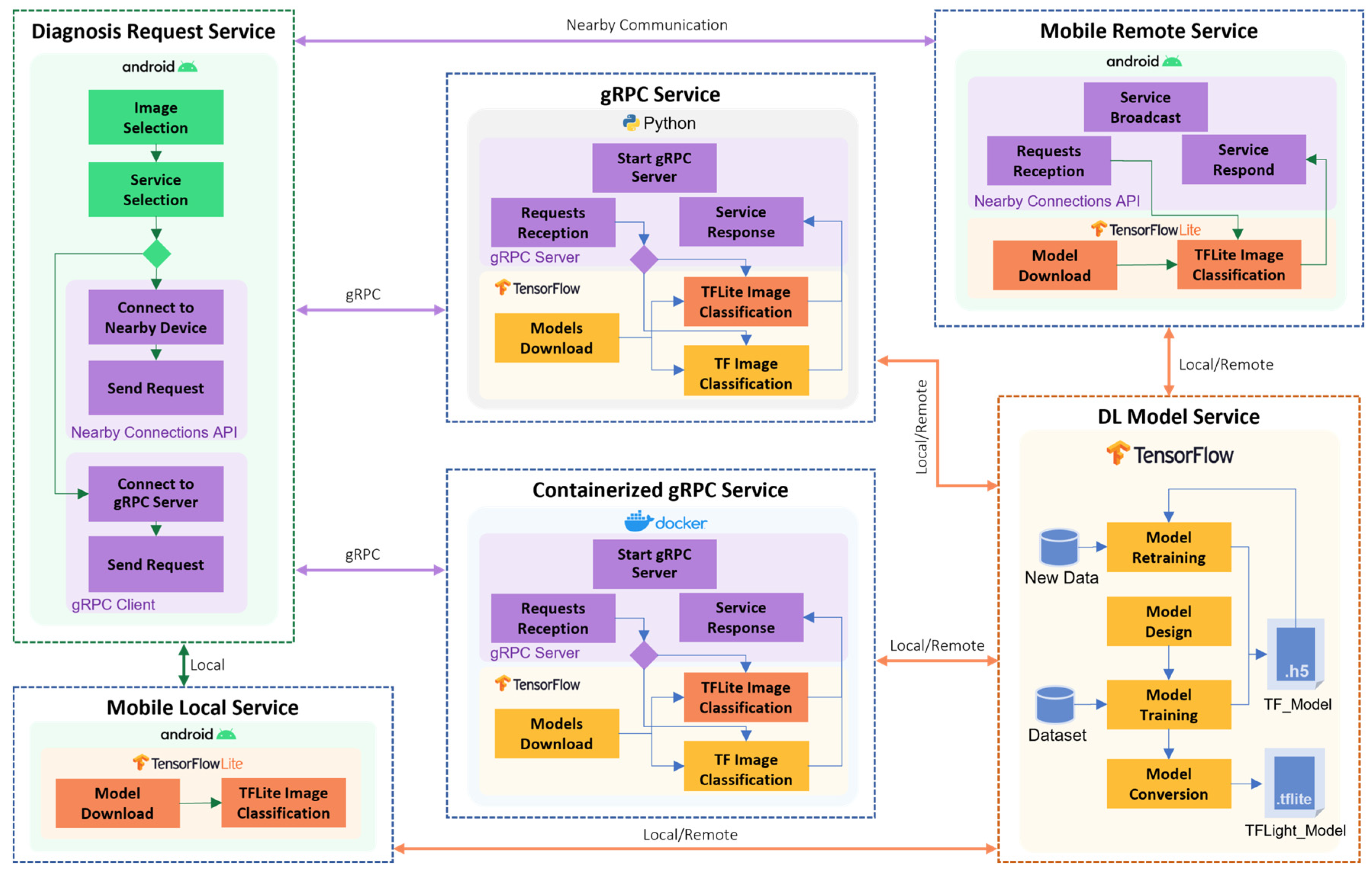
4.1. System Overview
| Algorithm 1: The Master Algorithm: Create_Services(skin_disease_diagnosis) |
| Input: ServiceClass skin_disease_diagnosis Output: service_catalog |
| 1 dataset_acquisition(skin_disease) 2 deep_learing_model_service ← design_deep_learing_model(tf_model, tf_lite_model) 3 instantiate(deep_learing_model_service) 4 service_catalog ← create_service_catalog (skin_disease_diagnosis) 5 mobile_local_service ← design_mobile_local (mobile) 6 instantiate (mobile_local_service) 7 mobile_remote_service ← design_mobile_remote (mobile) 8 instantiate (mobile_remote_service) 9 grpc_service ← design_grpc (pc, laptop, jetson, raspberry) 10 instantiate (grpc_service) 11 containerized_grpc_service ←design_container_grpc (cloud, pc, laptop) 12 instantiate (container_grpc_service) 13 diagnosis_request_service ←design_diagnosis_request (mobile, pc, laptop) 14 instantiate (diagnosis_request_service) |
| Algorithm 2: Diagnosis_Service |
| Input: skin_image Output: P[p0, …,pC] ∈ R //C is the number of skin disease classes |
| 1 Function: get_diagnosis (skin_image) 2 Init: size ← model input dimension, std ← model normalization factor //Image pre-processing 3 skin_image ← skin_image.rsize(size, size)//Resize the image to size x size 4 img_array[size, size] ← convert_to_array(skin_image)//Convert image to an array //Normalization 5 For x in img_array 6 For y in img_array[x] 7 img_array[x, y] ← img_array[x, y]/std 8 End For 9 End For //Classification 10 model ← load_model() //load trained model 11 P ← model.predict(img_array) 12 Return P |
4.2. Dataset
4.3. DL Models Service
| Algorithm 3: DL_Models_Service |
| Input: skin_image_dataset Output: tf_model, tf_lite_model files |
| 1 Function: design_models (skin_image_dataset) 2 Init: size ← input dimension, std ← normalization factor 3 tf_file_name ← “TF_model”, tf_lite_file_name ← “TFLite_model” //Model designing 4 tf_model ← design_tf_model() //Model training 5 For skin_image in skin_image_dataset //Image pre-processing 6 skin_image ← skin_image.rsize(size, size)//Resize the image to size x size 7 img_array[size, size] ← convert_to_array(skin_image)//Convert image to an array //Normalization 8 For x in img_array 9 For y in img_array[x] 10 img_array[x, y] ← img_array[x, y]/std 11 End For 12 End For 13 tf_model.train_model(img_array) 14 End For//end training //save TF model 15 tf_model.save_model(tf_file_name) //Convert to TFLite model 16 tf_lite_model ← convert_to_tflite(tf_model) 17 tf_lite_model.save_model(tf_lite_file_name) |
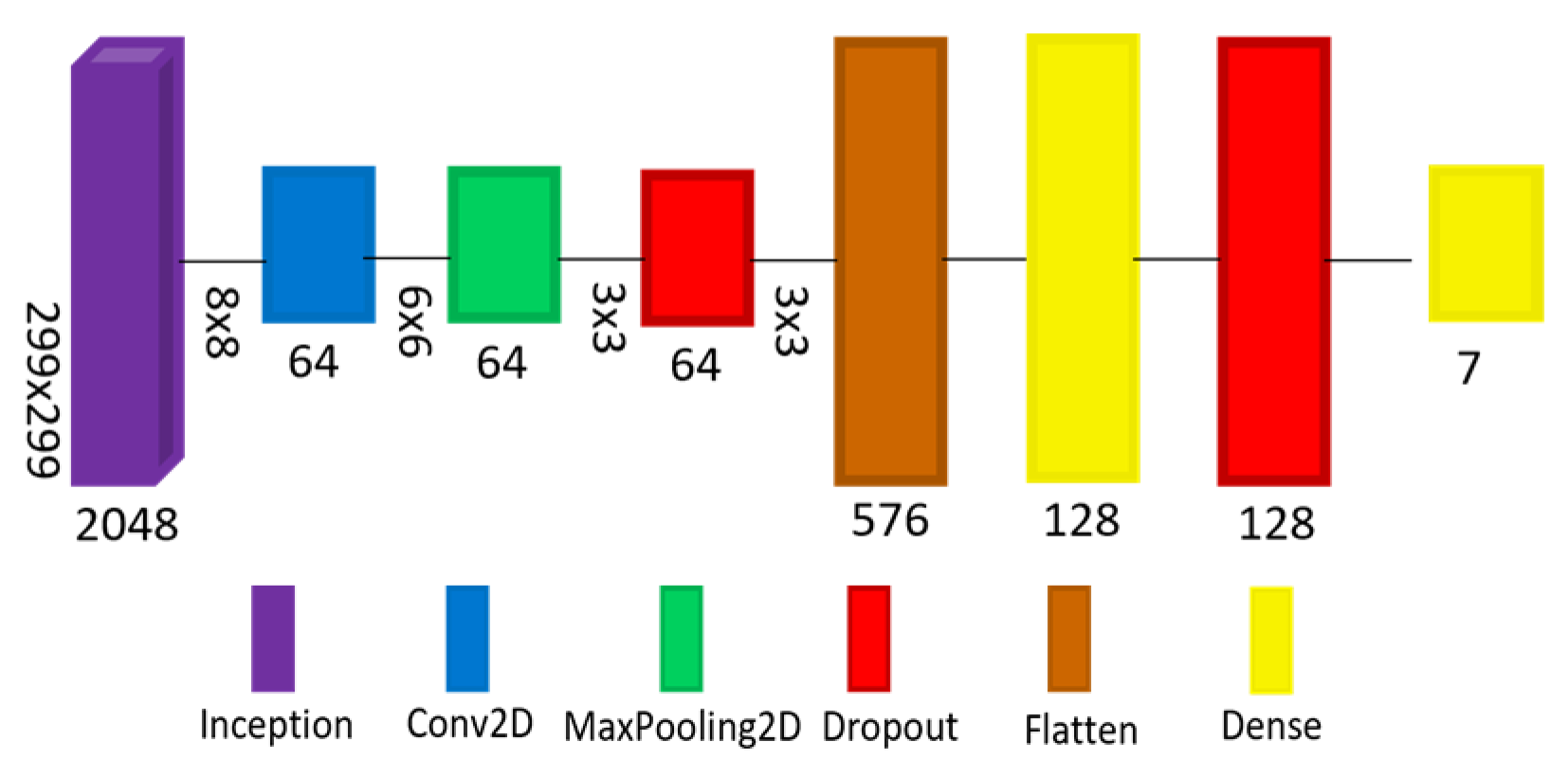
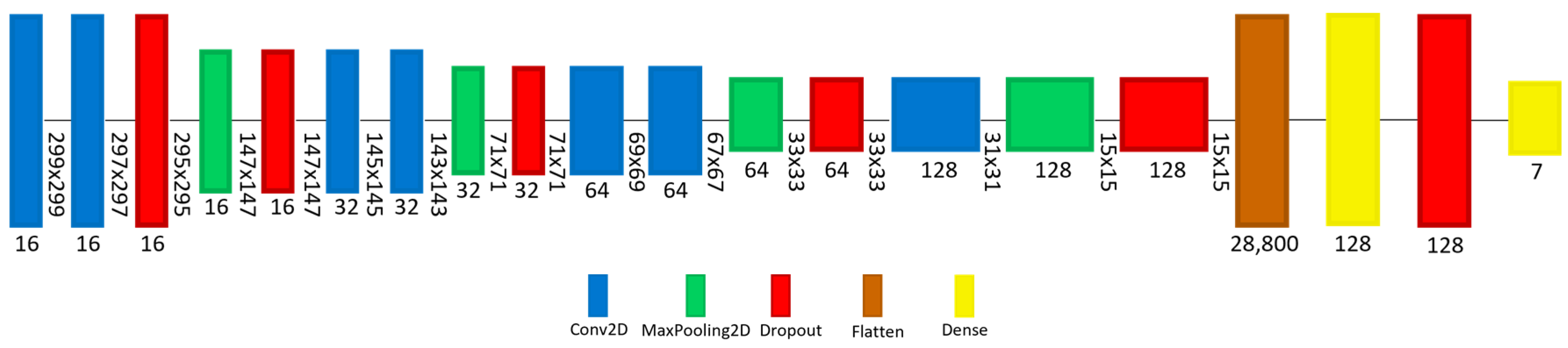
4.3.1. TensorFlow Model Design
4.3.2. TensorFlow Lite (TFLite) Model
4.4. Mobile Local Service
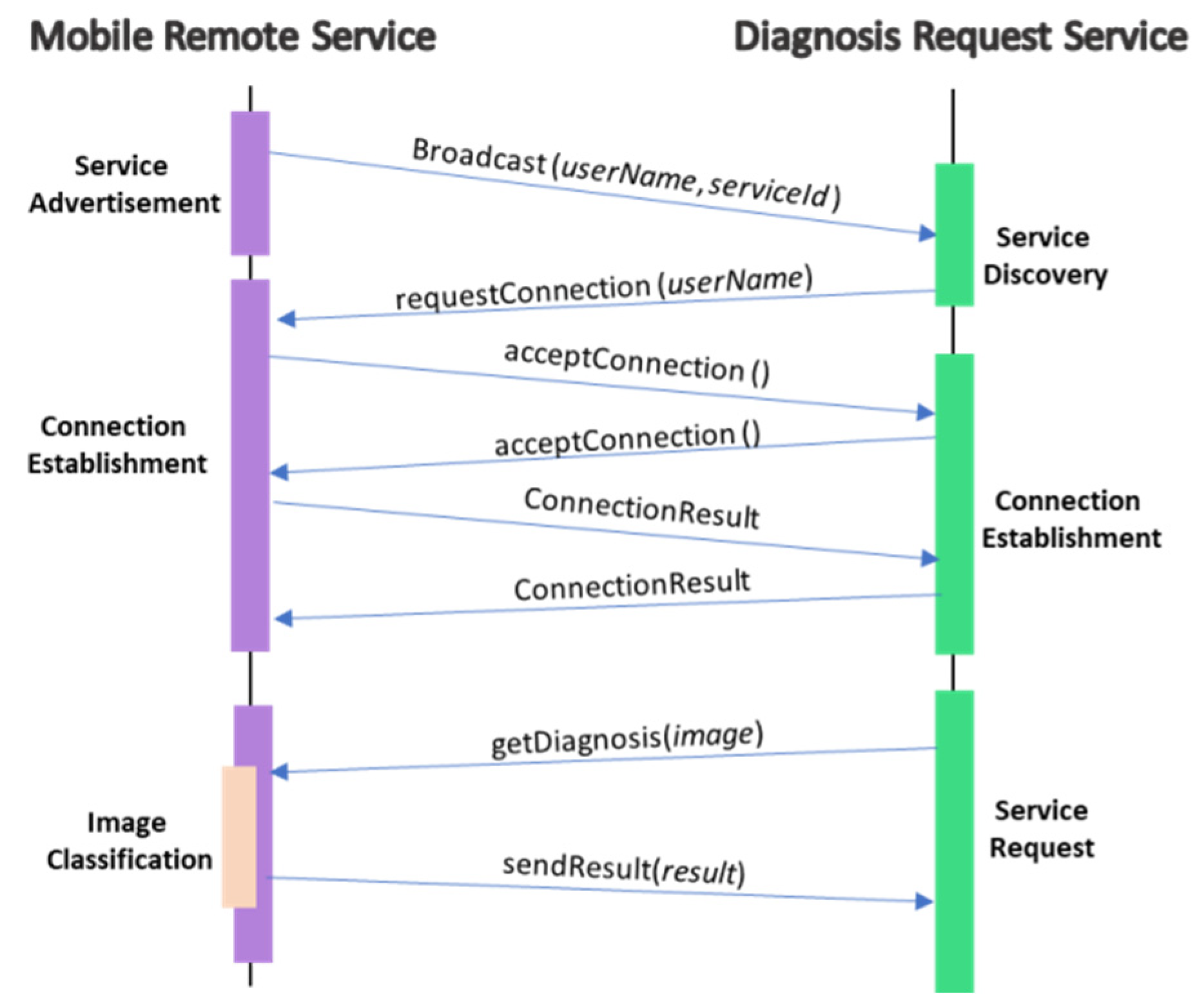
4.5. Mobile Remote Service
4.6. gRPC Service
4.7. Containerized gRPC Service
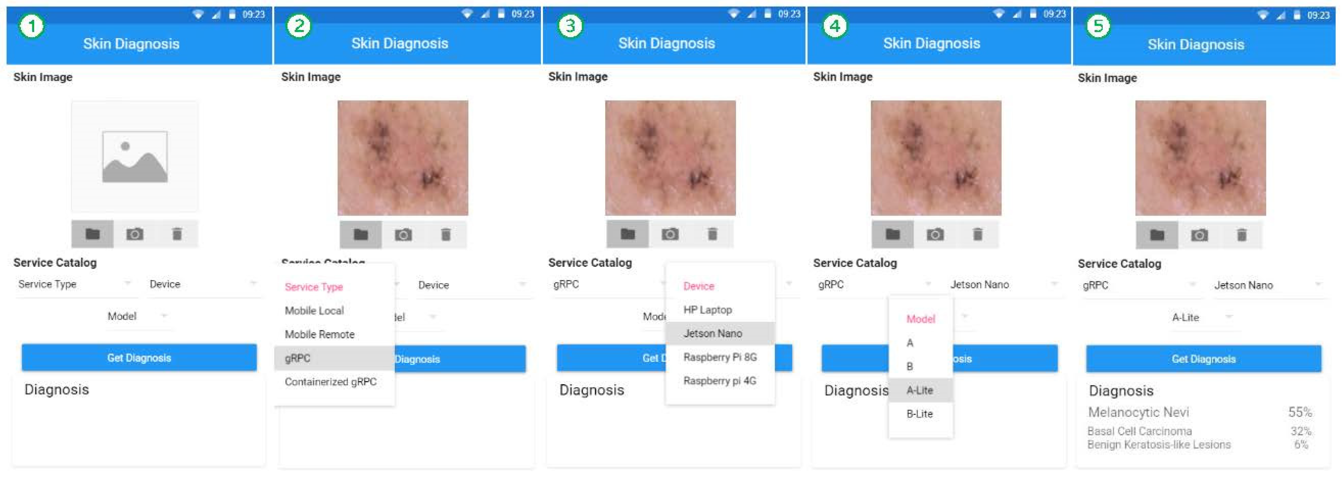
4.8. Diagnosis Request Service
| Algorithm 4: Diagnosis_Request_Service |
| Input: skin_image, service_type Output: class of skin disease |
| 1 Function: skin_diagnosis (skin_image, service_type) 2 Init: ip ← grpc server ip address, crt ← server certificate, url ← cloud service URL, 3 service_id ← nearby service ID, user_name ← given device name 4 Try 5 If service_type = = mobile_local_service Then //request from the local service 6 P[p0, … ,pC] ← mobile_local_service.get_diagnosis (skin_image) 7 Else If service_type = = mobile_remote_service Then //Create connection with the nearby device 8 connection ← request_connection(user_name) //Send a request to the diagnosis service 9 P[p0, … ,pC] ← connection.get_diagnosis (skin_image) 10 Else If service_type = = grpc_service Then //Create a secure channel with the diagnosis service 11 channel ← create_secure_channel (ip, crt) 12 P[p0, … ,pC] ← channel.get_diagnosis (skin_image) 13 Else If service_type = = containerized_grpc_service Then //Create a secure channel with the cloud 14 channel ← create_secure_channel (url) 15 P[p0, … ,pC] ← channel.get_diagnosis (skin_image) 16 End If //Find the largest probability value 17 probability ← p0 18 prediction_class ← 0 19 For c in C 20 If P[c] > probability Then 21 probability ← P[c] 22 prediction_class ← c 23 End If 24 End For //Find corresponding labels 25 prediction_label ← get_prediction_label(prediction_class) 26 Return prediction_label 27 Catch exception 28 Return error_message 29 End Try |
5. Service Evaluation and Analysis
5.1. Experimental Settings
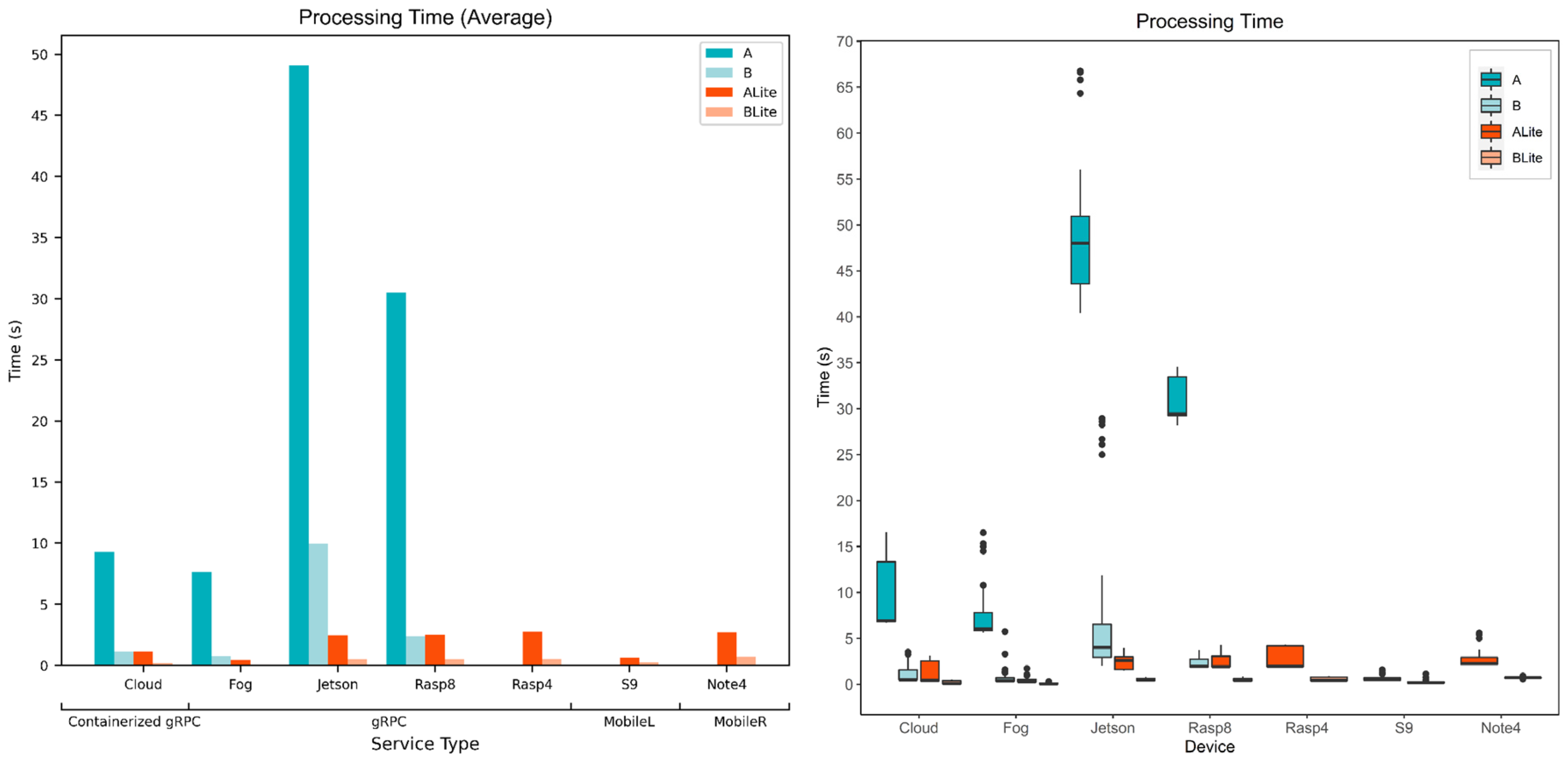
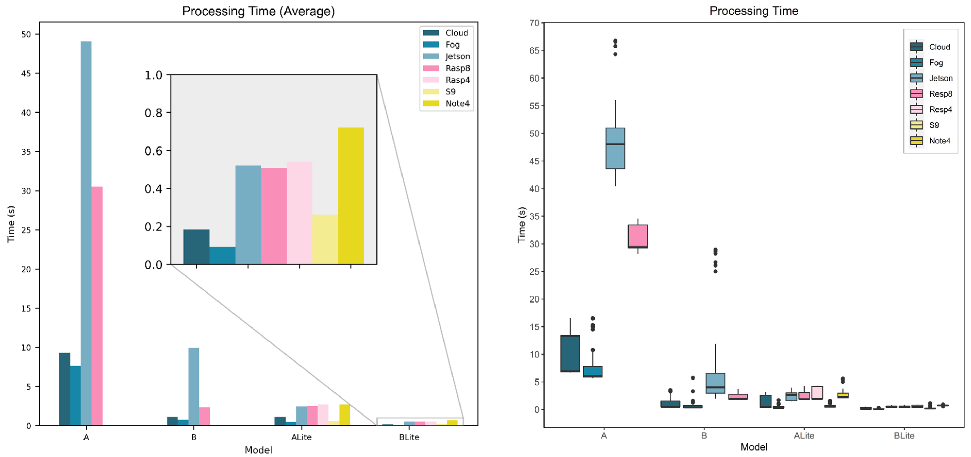
5.2. Service Processing Time
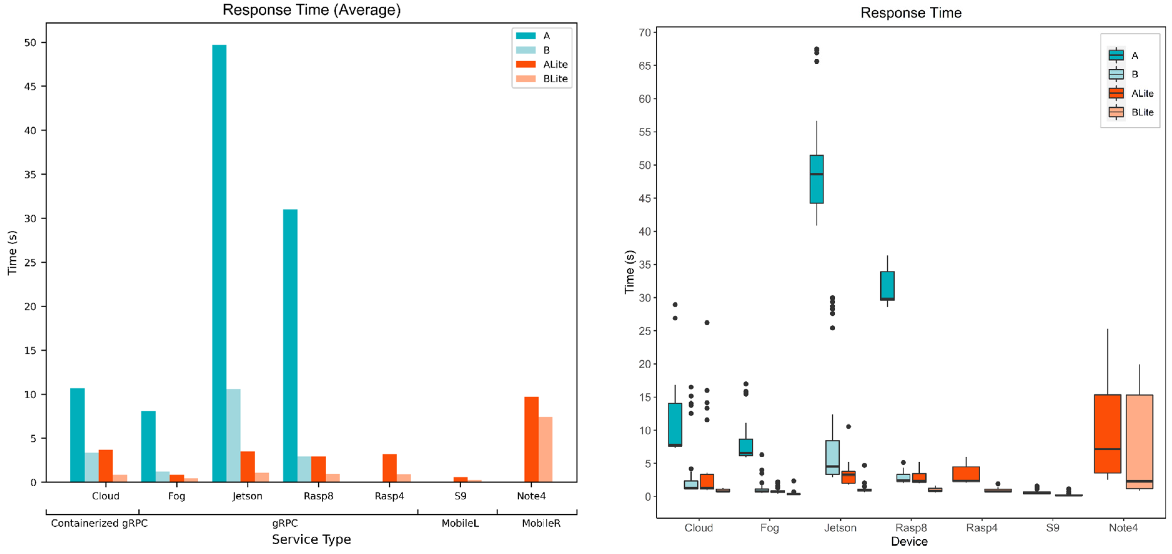
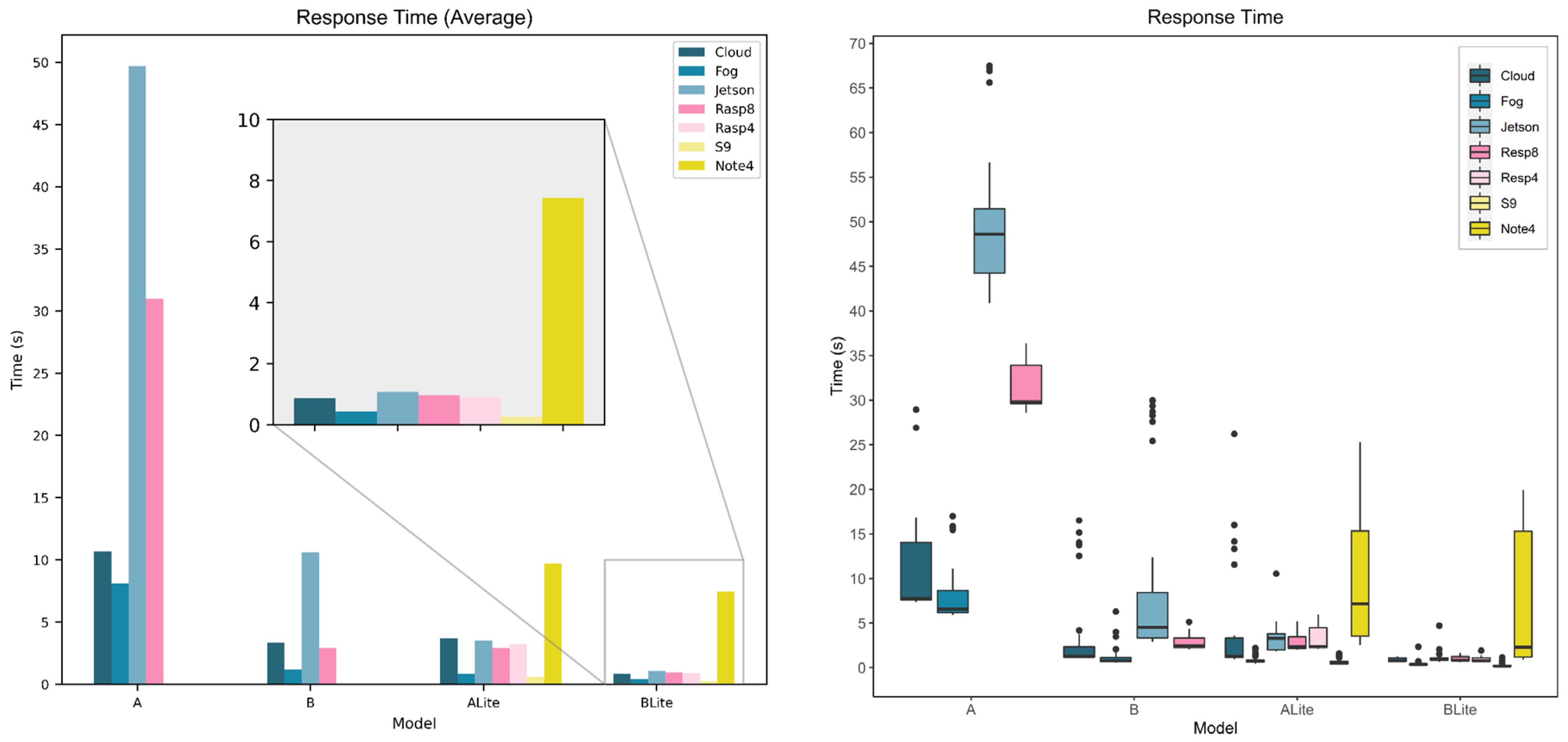
5.3. Service Response Time
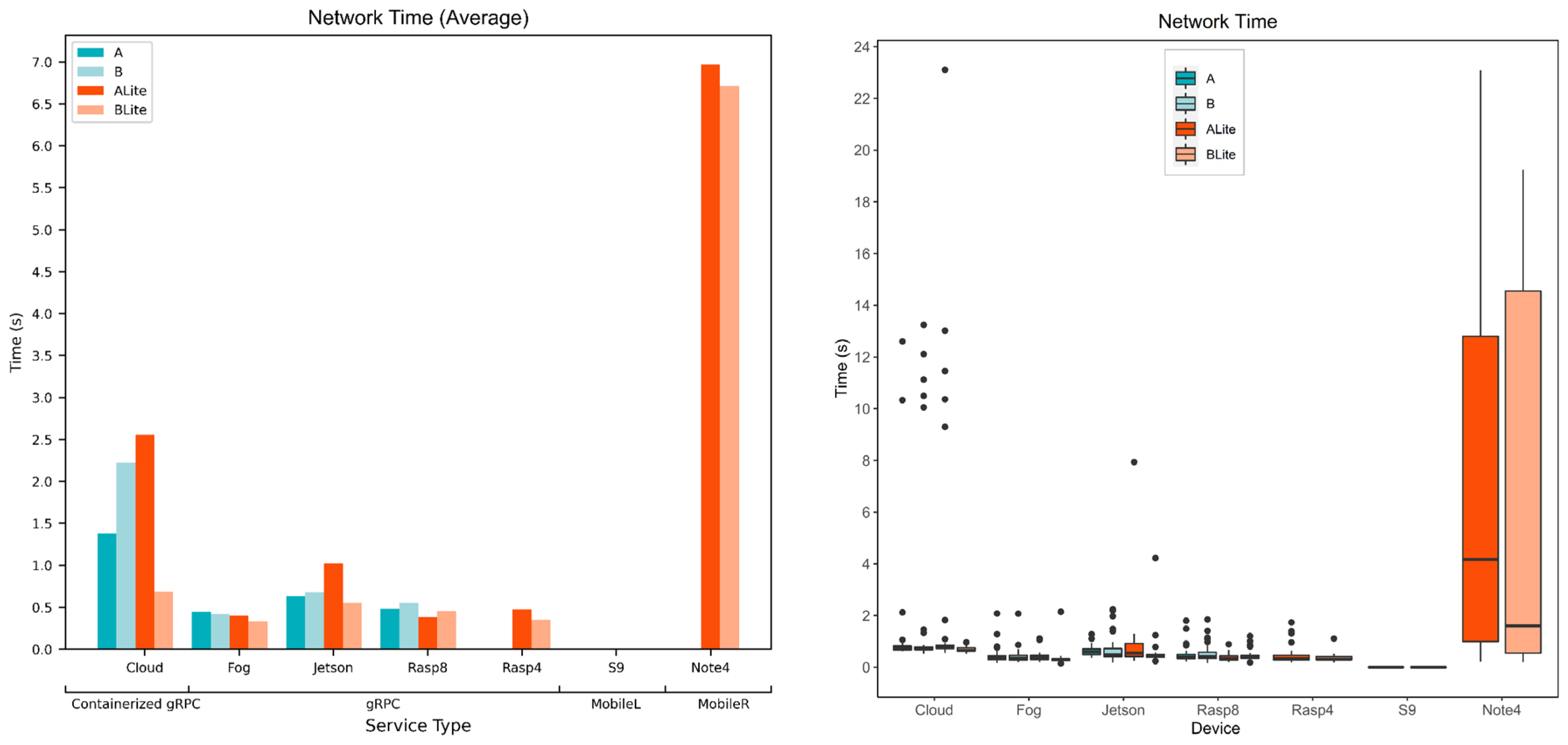
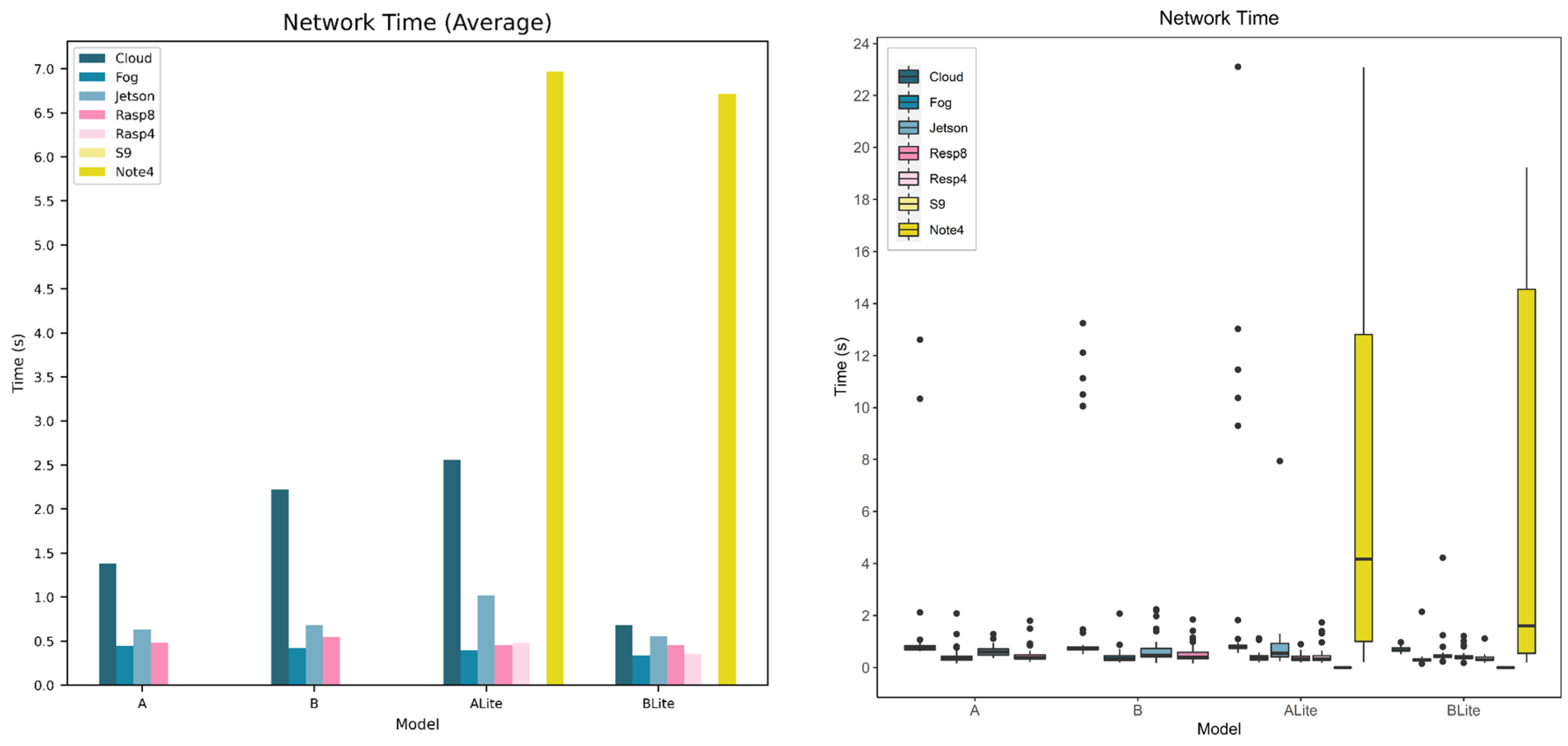
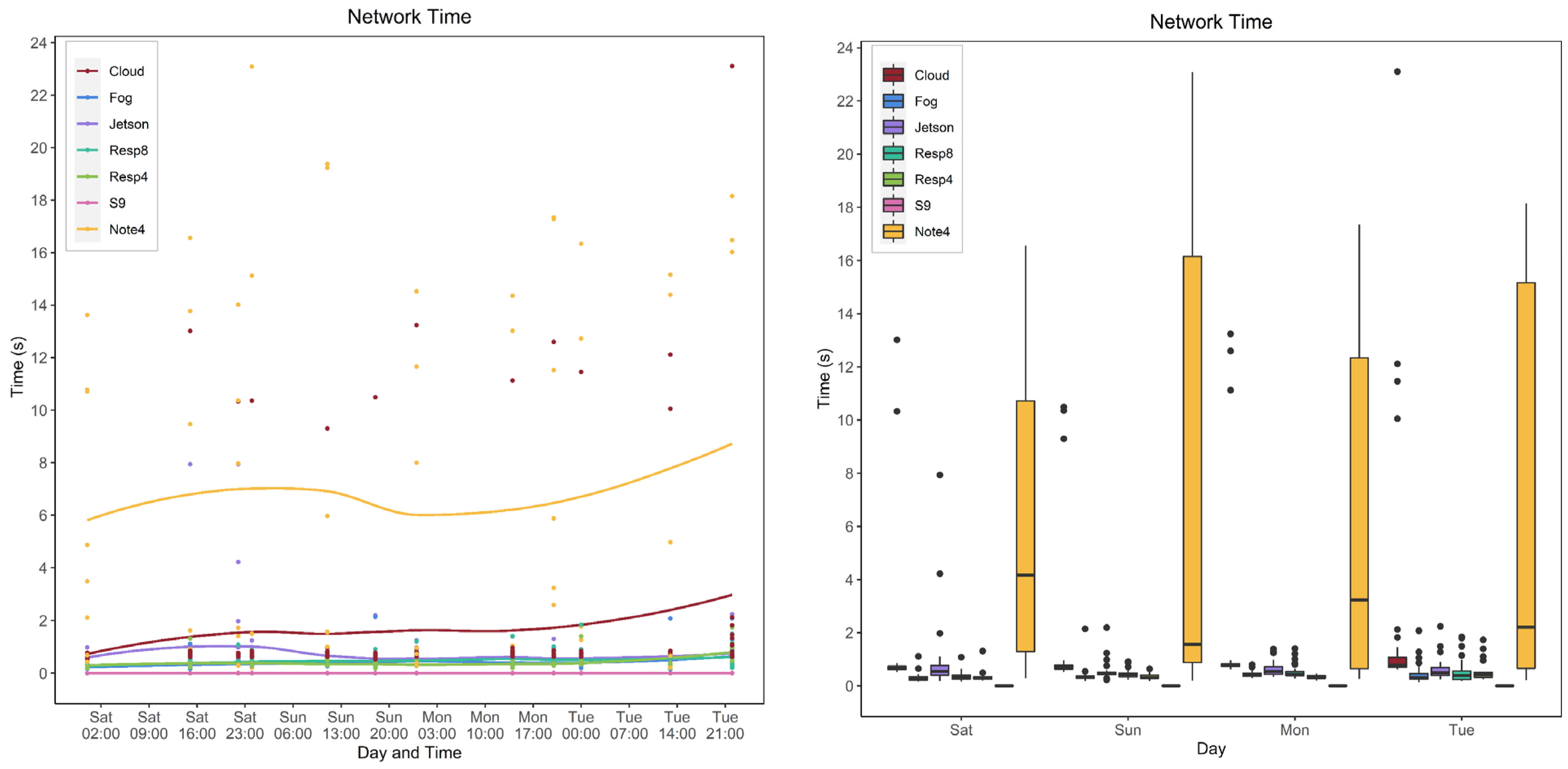
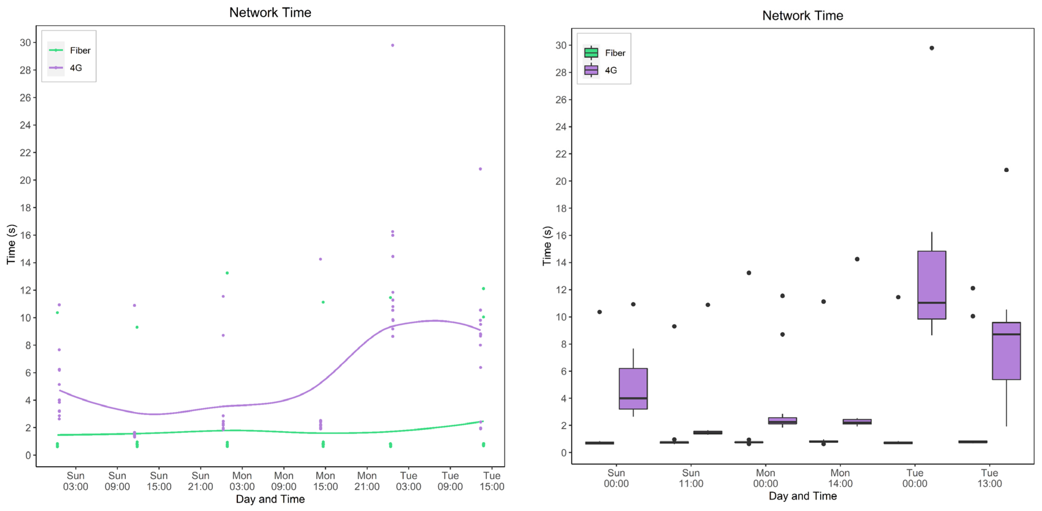
5.4. Service Network Time
5.4.1. Model and Device Behavior
5.4.2. Behavior over Weekdays
5.4.3. Cellular (4G) vs. Fiber Networks
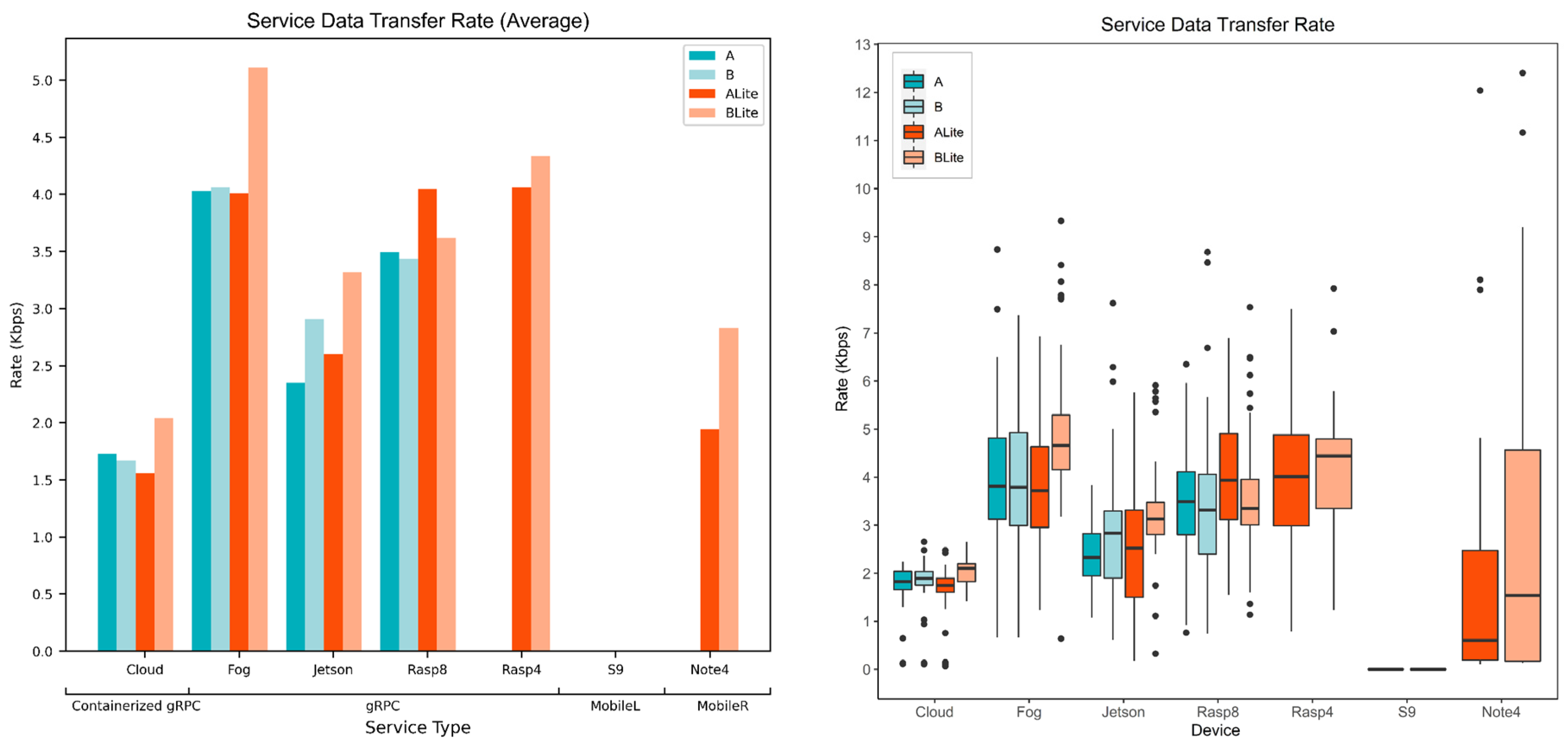
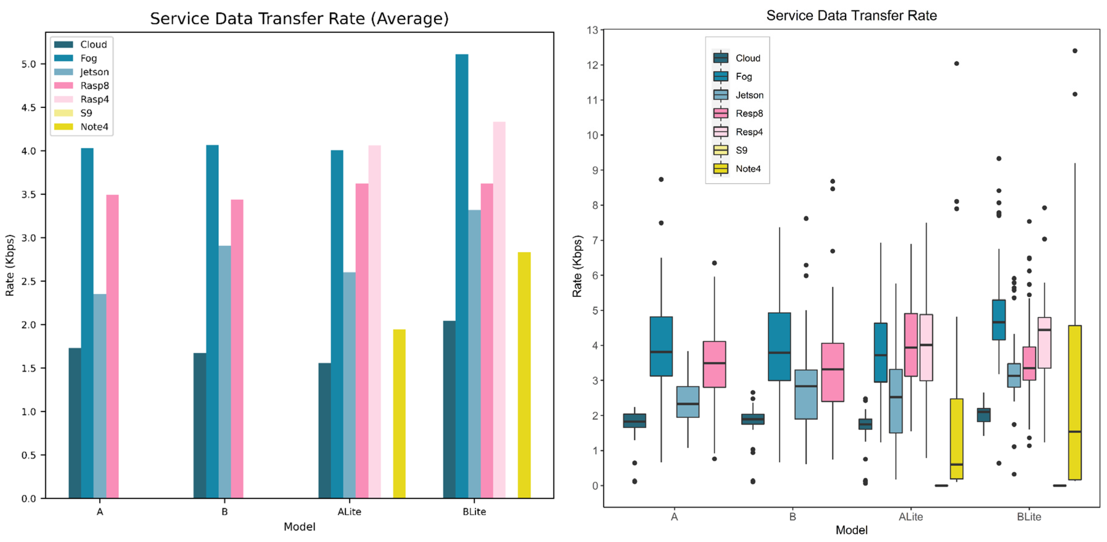
5.5. Service Data Transfer Rate
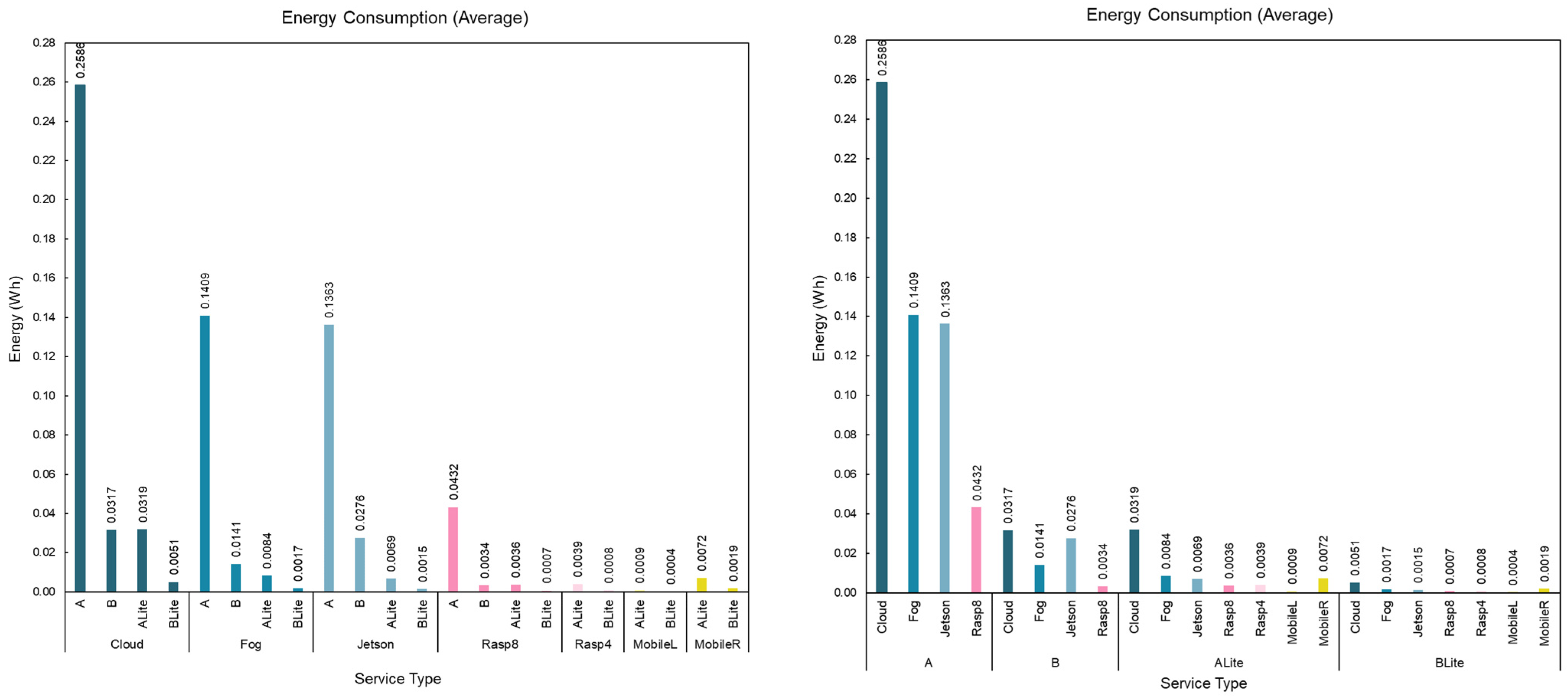
5.6. Service Energy Consumption
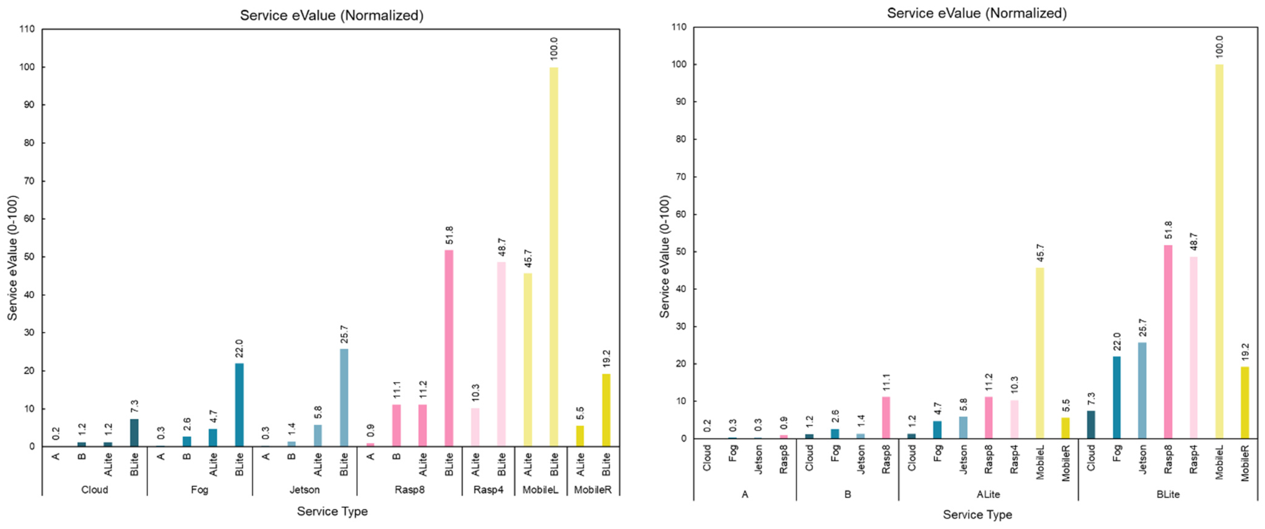
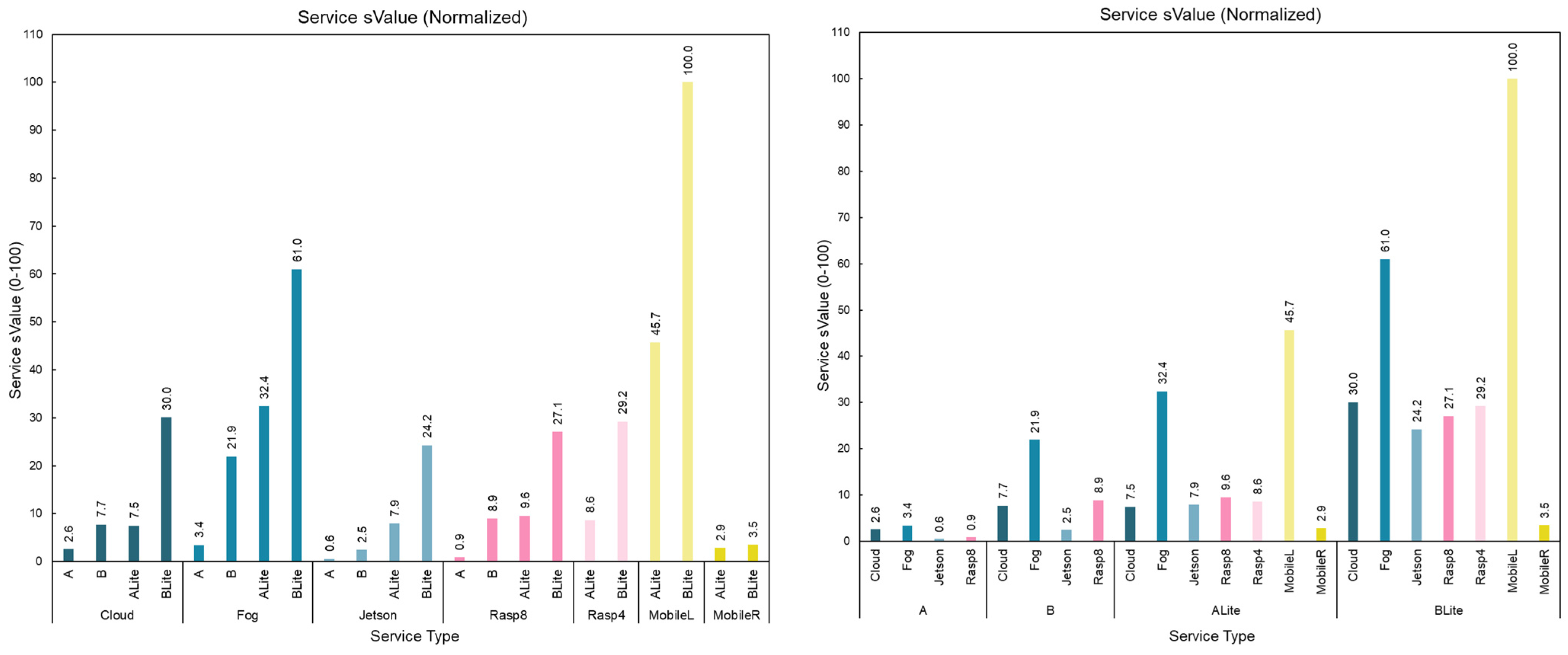
5.7. Service Value (eValue and sValue)
6. Conclusions and Future Work
Author Contributions
Funding
Institutional Review Board Statement
Informed Consent Statement
Data Availability Statement
Acknowledgments
Conflicts of Interest
References
- Mehmood, R.; Alam, F.; Albogami, N.N.; Katib, I.; Albeshri, A.; Altowaijri, S.M. UTiLearn: A Personalised Ubiquitous Teaching and Learning System for Smart Societies. IEEE Access 2017, 5, 2615–2635. [Google Scholar] [CrossRef]
- Yigitcanlar, T.; Butler, L.; Windle, E.; Desouza, K.C.; Mehmood, R.; Corchado, J.M. Can Building ‘Artificially Intelligent Cities’ Safeguard Humanity from Natural Disasters, Pandemics, and Other Catastrophes? An Urban Scholar’s Perspective. Sensors 2020, 20, 2988. [Google Scholar] [CrossRef] [PubMed]
- Yigitcanlar, T.; Kankanamge, N.; Regona, M.; Maldonado, A.; Rowan, B.; Ryu, A.; DeSouza, K.C.; Corchado, J.M.; Mehmood, R.; Li, R.Y.M. Artificial Intelligence Technologies and Related Urban Planning and Development Concepts: How Are They Perceived and Utilized in Australia? J. Open Innov. Technol. Mark. Complex. 2020, 6, 187. [Google Scholar] [CrossRef]
- AlOmari, E.; Katib, I.; Albeshri, A.; Mehmood, R. COVID-19: Detecting Government Pandemic Measures and Public Concerns from Twitter Arabic Data Using Distributed Machine Learning. Int. J. Environ. Res. Public Health 2021, 18, 282. [Google Scholar] [CrossRef] [PubMed]
- Yigitcanlar, T.; Corchado, J.; Mehmood, R.; Li, R.; Mossberger, K.; Desouza, K. Responsible Urban Innovation with Local Government Artificial Intelligence (AI): A Conceptual Framework and Research Agenda. J. Open Innov. Technol. Mark. Complex. 2021, 7, 71. [Google Scholar] [CrossRef]
- Alotaibi, S.; Mehmood, R.; Katib, I.; Rana, O.; Albeshri, A. Sehaa: A Big Data Analytics Tool for Healthcare Symptoms and Diseases Detection Using Twitter, Apache Spark, and Machine Learning. Appl. Sci. 2020, 10, 1398. [Google Scholar] [CrossRef] [Green Version]
- Yigitcanlar, T.; Mehmood, R.; Corchado, J.M. Green Artificial Intelligence: Towards an Efficient, Sustainable and Equitable Technology for Smart Cities and Futures. Sustainability 2021, 13, 8952. [Google Scholar] [CrossRef]
- Alam, F.; Mehmood, R.; Katib, I.; Albogami, N.N.; Albeshri, A. Data Fusion and IoT for Smart Ubiquitous Environments: A Survey. IEEE Access 2017, 5, 9533–9554. [Google Scholar] [CrossRef]
- Mehmood, R.; Faisal, M.A.; Altowaijri, S. Future networked healthcare systems: A review and case study. In Handbook of Research on Redesigning the Future of Internet Architectures; IGI Global: Hershey, PA, USA, 2015; pp. 531–555. [Google Scholar]
- Greco, L.; Percannella, G.; Ritrovato, P.; Tortorella, F.; Vento, M. Trends in IoT based solutions for health care: Moving AI to the edge. Pattern Recognit. Lett. 2020, 135, 346–353. [Google Scholar] [CrossRef]
- Mukherjee, A.; Ghosh, S.; Behere, A.; Ghosh, S.K.; Buyya, R. Internet of Health Things (IoHT) for personalized health care using integrated edge-fog-cloud network. J. Ambient Intell. Humaniz. Comput. 2020, 12, 943–959. [Google Scholar] [CrossRef]
- Farahani, B.; Barzegari, M.; Aliee, F.S.; Shaik, K.A. Towards collaborative intelligent IoT eHealth: From device to fog, and cloud. Microprocess. Microsyst. 2019, 72, 102938. [Google Scholar] [CrossRef]
- Janbi, N.; Katib, I.; Albeshri, A.; Mehmood, R. Distributed Artificial Intelligence-as-a-Service (DAIaaS) for Smarter IoE and 6G Environments. Sensors 2020, 20, 5796. [Google Scholar] [CrossRef] [PubMed]
- Usman, S.; Mehmood, R.; Katib, I. Big Data and HPC Convergence for Smart Infrastructures: A Review and Proposed Architecture. Smart Infrastruct. Appl. 2020, 561–586. [Google Scholar]
- Al-Dhubhani, R.; Mehmood, R.; Katib, I.; Algarni, A. Location privacy in smart cities era. In Lecture Notes of the Institute for Computer Sciences, Social-Informatics and Telecommunications Engineering; Springer Publishing Company: New York, NY, USA, 2018; Volume 224, pp. 123–138. [Google Scholar]
- Assiri, F.Y.; Mehmood, R. Software Quality in the Era of Big Data, IoT and Smart Cities; Springer: Cham, Switzerland, 2020; pp. 519–536. [Google Scholar]
- Singh, J.; Kad, S.; Singh, P.D. Implementing Fog Computing for Detecting Primary Tumors Using Hybrid Approach of Data Mining; Springer: Singapore, 2021; pp. 1067–1080. [Google Scholar]
- Amin, S.U.; Hossain, M.S. Edge Intelligence and Internet of Things in Healthcare: A Survey. IEEE Access 2020, 9, 45–59. [Google Scholar] [CrossRef]
- Arfat, Y.; Aqib, M.; Mehmood, R.; Albeshri, A.; Katib, I.; Albogami, N.; Alzahrani, A. Enabling Smarter Societies through Mobile Big Data Fogs and Clouds. Procedia Comput. Sci. 2017, 109, 1128–1133. [Google Scholar] [CrossRef]
- Arfat, Y.; Usman, S.; Mehmood, R.; Katib, I. Big Data for Smart Infrastructure Design: Opportunities and Challenges. Smart Infrastruct. Appl. 2020, 491–518. [Google Scholar]
- Ahmad, A.; Fahmideh, M.; Altamimi, A.B.; Katib, I.; Albeshri, A.; Alreshidi, A.; Mehmood, R. Software Engineering for IoT-Driven Data Analytics Applications. IEEE Access 2021, 9, 48197–48217. [Google Scholar] [CrossRef]
- Tang, P.; Dong, Y.; Chen, Y.; Mao, S.; Halgamuge, S. QoE-Aware Traffic Aggregation Using Preference Logic for Edge Intelligence. IEEE Trans. Wirel. Commun. 2021, 20, 6093–6106. [Google Scholar] [CrossRef]
- Tsaur, W.-J.; Yeh, L.-Y. DANS: A Secure and Efficient Driver-Abnormal Notification Scheme With IoT Devices Over IoV. IEEE Syst. J. 2018, 13, 1628–1639. [Google Scholar] [CrossRef]
- Cui, X.; Zhang, W.; Finkler, U.; Saon, G.; Picheny, M.; Kung, D. Distributed Training of Deep Neural Network Acoustic Models for Automatic Speech Recognition: A comparison of current training strategies. IEEE Signal Process. Mag. 2020, 37, 39–49. [Google Scholar] [CrossRef]
- Langer, M.; He, Z.; Rahayu, W.; Xue, Y. Distributed Training of Deep Learning Models: A Taxonomic Perspective. IEEE Trans. Parallel Distrib. Syst. 2020, 31, 2802–2818. [Google Scholar] [CrossRef]
- Aspri, M.; Tsagkatakis, G.; Tsakalides, P. Distributed Training and Inference of Deep Learning Models for Multi-Modal Land Cover Classification. Remote Sens. 2020, 12, 2670. [Google Scholar] [CrossRef]
- Sugi, S.S.S.; Ratna, S.R. A novel distributed training on fog node in IoT backbone networks for security. Soft Comput. 2020, 24, 18399–18410. [Google Scholar] [CrossRef]
- Li, C.; Wang, S.; Li, X.; Zhao, F.; Yu, R. Distributed perception and model inference with intelligent connected vehicles in smart cities. Ad Hoc Netw. 2020, 103, 102152. [Google Scholar] [CrossRef]
- Hosseinalipour, S.; Brinton, C.G.; Aggarwal, V.; Dai, H.; Chiang, M. From Federated to Fog Learning: Distributed Machine Learning over Heterogeneous Wireless Networks. IEEE Commun. Mag. 2020, 58, 41–47. [Google Scholar] [CrossRef]
- Zhou, Z.; Chen, X.; Li, E.; Zeng, L.; Luo, K.; Zhang, J. Edge Intelligence: Paving the Last Mile of Artificial Intelligence With Edge Computing. Proc. IEEE 2019, 8, 1738–1762. [Google Scholar] [CrossRef] [Green Version]
- Cao, Y.; Chen, S.; Hou, P.; Brown, D. FAST: A fog computing assisted distributed analytics system to monitor fall for stroke mitigation. In Proceedings of the 2015 IEEE International Conference on Networking, Architecture and Storage, NAS 2015, Boston, MA, USA, 6–7 August 2015; pp. 2–11. [Google Scholar]
- Hassan, S.R.; Ahmad, I.; Ahmad, S.; AlFaify, A.; Shafiq, M. Remote Pain Monitoring Using Fog Computing for e-Healthcare: An Efficient Architecture. Sensors 2020, 20, 6574. [Google Scholar] [CrossRef]
- Mohammed, T.; Albeshri, A.; Katib, I.; Mehmood, R. UbiPriSEQ—Deep reinforcement learning to manage privacy, security, energy, and QoS in 5G IoT hetnets. Appl. Sci. 2020, 10, 7120. [Google Scholar] [CrossRef]
- Deng, S.; Zhao, H.; Fang, W.; Yin, J.; Dustdar, S.; Zomaya, A.Y. Edge Intelligence: The Confluence of Edge Computing and Artificial Intelligence. IEEE Internet Things J. 2020, 7, 7457–7469. [Google Scholar] [CrossRef] [Green Version]
- Wang, X.; Han, Y.; Leung, V.C.M.; Niyato, D.; Yan, X.; Chen, X. Convergence of Edge Computing and Deep Learning: A Comprehensive Survey. IEEE Commun. Surv. Tutorials 2020, 22, 869–904. [Google Scholar] [CrossRef] [Green Version]
- Park, J.; Samarakoon, S.; Bennis, M.; Debbah, M. Wireless Network Intelligence at the Edge. Proc. IEEE 2019, 107, 2204–2239. [Google Scholar] [CrossRef] [Green Version]
- Chen, J.; Ran, X. Deep Learning With Edge Computing: A Review. Proc. IEEE 2019, 107, 1655–1674. [Google Scholar] [CrossRef]
- Isakov, M.; Gadepally, V.; Gettings, K.M.; Kinsy, M.A. Survey of Attacks and Defenses on Edge-Deployed Neural Networks. In Proceedings of the 2019 IEEE High Performance Extreme Computing Conference (HPEC), Waltham, MA, USA, 24–26 September 2019; pp. 1–8. [Google Scholar]
- Rausch, T.; Dustdar, S. Edge intelligence: The convergence of humans, things, and AI. In Proceedings of the 2019 IEEE International Conference on Cloud Engineering, IC2E 2019, Prague, Czech Republic, 24–27 June 2019; pp. 86–96. [Google Scholar]
- Shi, Z. Advanced Artificial Intelligence, 2nd ed.; World Scientific: Singapore, 2019. [Google Scholar]
- Pattnaik, B.S.; Pattanayak, A.S.; Udgata, S.K.; Panda, A.K. Advanced centralized and distributed SVM models over different IoT levels for edge layer intelligence and control. Evol. Intell. 2020, 1–15. [Google Scholar] [CrossRef]
- Gao, Y.; Liu, L.; Zheng, X.; Zhang, C.; Ma, H. Federated Sensing: Edge-Cloud Elastic Collaborative Learning for Intelligent Sensing. IEEE Internet Things J. 2021, 8, 11100–11111. [Google Scholar] [CrossRef]
- Chen, Y.; Qin, X.; Wang, J.; Yu, C.; Gao, W. FedHealth: A Federated Transfer Learning Framework for Wearable Healthcare. IEEE Intell. Syst. 2020, 35, 83–93. [Google Scholar] [CrossRef] [Green Version]
- Hegedűs, I.; Danner, G.; Jelasity, M. Decentralized learning works: An empirical comparison of gossip learning and federated learning. J. Parallel Distrib. Comput. 2020, 148, 109–124. [Google Scholar] [CrossRef]
- Kim, H.; Park, J.; Bennis, M.; Kim, S.-L. Blockchained On-Device Federated Learning. IEEE Commun. Lett. 2019, 24, 1279–1283. [Google Scholar] [CrossRef] [Green Version]
- TensorFlow Lite | ML for Mobile and Edge Devices. Available online: https://www.tensorflow.org/lite (accessed on 12 October 2020).
- Zebin, T.; Scully, P.J.; Peek, N.; Casson, A.J.; Ozanyan, K.B. Design and Implementation of a Convolutional Neural Network on an Edge Computing Smartphone for Human Activity Recognition. IEEE Access 2019, 7, 133509–133520. [Google Scholar] [CrossRef]
- Benhamida, A.; Varkonyi-Koczy, A.R.; Kozlovszky, M. Traffic Signs Recognition in a mobile-based application using TensorFlow and Transfer Learning technics. In Proceedings of the 2020 IEEE 15th International Conference of System of Systems Engineering (SoSE), Budapest, Hungary, 2–4 June 2020; pp. 000537–000542. [Google Scholar]
- Alsing, O. Mobile Object Detection Using TensorFlow Lite and Transfer Learning; KTH Royal Institute of Technology: Stockholm, Sweden, 2018. [Google Scholar]
- Zeroual, A.; Derdour, M.; Amroune, M.; Bentahar, A. Using a Fine-Tuning Method for a Deep Authentication in Mobile Cloud Computing Based on Tensorflow Lite Framework. In Proceedings of the ICNAS 2019: 4th International Conference on Networking and Advanced Systems, Annaba, Algeria, 26–27 June 2019. [Google Scholar]
- Ahmadi, M.; Sotgiu, A.; Giacinto, G. IntelliAV: Toward the feasibility of building intelligent anti-malware on android devices. In Proceedings of the Lecture Notes in Computer Science (Including Subseries Lecture Notes in Artificial Intelligence and Lecture Notes in Bioinformatics), Reggio, Italy, 29 August–1 September 2017; Volume 10410, pp. 137–154. [Google Scholar]
- Soltani, N.; Sankhe, K.; Ioannidis, S.; Jaisinghani, D.; Chowdhury, K. Spectrum Awareness at the Edge: Modulation Classification using Smartphones. In Proceedings of the 2019 IEEE International Symposium on Dynamic Spectrum Access Networks, DySPAN 2019, Newark, NJ, USA, 11–14 November 2019. [Google Scholar]
- Domozi, Z.; Stojcsics, D.; Benhamida, A.; Kozlovszky, M.; Molnar, A. Real time object detection for aerial search and rescue missions for missing persons. In Proceedings of the 2020 IEEE 15th International Conference of System of Systems Engineering (SoSE), Budapest, Hungary, 2–4 June 2020; pp. 000519–000524. [Google Scholar]
- Caffe2 Deep Learning Framework | NVIDIA Developer. Available online: https://developer.nvidia.com/caffe2 (accessed on 12 October 2020).
- Home | PyTorch. Available online: https://pytorch.org/mobile/home/ (accessed on 12 October 2020).
- Muhammed, T.; Mehmood, R.; Albeshri, A.; Katib, I. UbeHealth: A Personalized Ubiquitous Cloud and Edge-Enabled Networked Healthcare System for Smart Cities. IEEE Access 2018, 6, 32258–32285. [Google Scholar] [CrossRef]
- Goyal, M.; Knackstedt, T.; Yan, S.; Hassanpour, S. Artificial intelligence-based image classification methods for diagnosis of skin cancer: Challenges and opportunities. Comput. Biol. Med. 2020, 127, 104065. [Google Scholar] [CrossRef]
- Skin Cancer Facts & Statistics—The Skin Cancer Foundation. Available online: https://www.skincancer.org/skin-cancer-information/skin-cancer-facts/ (accessed on 24 March 2020).
- Bray, F.; Ferlay, J.; Soerjomataram, I.; Siegel, R.L.; Torre, L.A.; Jemal, A. Global cancer statistics 2018: GLOBOCAN estimates of incidence and mortality worldwide for 36 cancers in 185 countries. CA Cancer J. Clin. 2018, 68, 394–424. [Google Scholar] [CrossRef] [PubMed] [Green Version]
- Claudiu, P.; Ion, B.; Tudorel, P.; Iordache, I.; Nida, B.; Abdulazis, T.; Panculescu, F. The Value of Digital Dermatoscopy in the Diagnosis and Treatment of Precancerous Skin Lesions. ARS Med. Tomitana 2018, 24, 40–45. [Google Scholar] [CrossRef] [Green Version]
- Ashique, K.T.; Aurangabadkar, S.J.; Kaliyadan, F. Clinical photography in dermatology using smartphones: An overview. Indian Dermatol. Online J. 2015, 6, 158–163. [Google Scholar] [CrossRef] [PubMed]
- Sonthalia, S.; Kaliyadan, F. Dermoscopy Overview and Extradiagnostic Applications; StatPearls Publishing: Treasure Island, FL, USA, 2020. [Google Scholar]
- Jha, D.; Riegler, M.A.; Johansen, D.; Halvorsen, P.; Johansen, H.D. DoubleU-Net: A Deep Convolutional Neural Network for Medical Image Segmentation. In Proceedings of the IEEE Symposium on Computer-Based Medical Systems, Rochester, MA, USA, 28–30 July 2020; pp. 558–564. [Google Scholar]
- Bajwa, M.N.; Muta, K.; Malik, M.I.; Siddiqui, S.A.; Braun, S.A.; Homey, B.; Dengel, A.; Ahmed, S. Computer-Aided Diagnosis of Skin Diseases Using Deep Neural Networks. Appl. Sci. 2020, 10, 2488. [Google Scholar] [CrossRef] [Green Version]
- Zhang, X.; Wang, S.; Liu, J.; Tao, C. Towards improving diagnosis of skin diseases by combining deep neural network and human knowledge. BMC Med Informatics Decis. Mak. 2018, 18, 69–76. [Google Scholar] [CrossRef] [Green Version]
- Wei, L.-S.; Gan, Q.; Ji, T. Skin Disease Recognition Method Based on Image Color and Texture Features. Comput. Math. Methods Med. 2018, 2018, 1–10. [Google Scholar] [CrossRef] [Green Version]
- Liu, Y.; Jain, A.; Eng, C.; Way, D.H.; Lee, K.; Bui, P.; Kanada, K.; Marinho, G.D.O.; Gallegos, J.; Gabriele, S.; et al. A deep learning system for differential diagnosis of skin diseases. Nat. Med. 2020, 26, 900–908. [Google Scholar] [CrossRef]
- Gavrilov, D.A.; Melerzanov, A.V.; Shchelkunov, N.N.; Zakirov, E.I. Use of Neural Network-Based Deep Learning Techniques for the Diagnostics of Skin Diseases. Biomed. Eng. 2019, 52, 348–352. [Google Scholar] [CrossRef]
- Goyal, M.; Oakley, A.; Bansal, P.; Dancey, D.; Yap, M.H. Skin Lesion Segmentation in Dermoscopic Images With Ensemble Deep Learning Methods. IEEE Access 2019, 8, 4171–4181. [Google Scholar] [CrossRef]
- Ünver, H.M.; Ayan, E. Skin Lesion Segmentation in Dermoscopic Images with Combination of YOLO and GrabCut Algorithm. Diagnostics 2019, 9, 72. [Google Scholar] [CrossRef] [Green Version]
- He, X.; Wang, S.; Shi, S.; Tang, Z.; Wang, Y.; Zhao, Z.; Chu, X. Computer-Aided Clinical Skin Disease Diagnosis Using CNN and Object Detection Models. In Proceedings of the 2019 IEEE International Conference on Big Data, Big Data 2019, Los Angeles, CA, USA, 9–12 December 2019; pp. 4839–4844. [Google Scholar]
- Garcia-Arroyo, J.L.; Garcia-Zapirain, B. Segmentation of skin lesions in dermoscopy images using fuzzy classification of pixels and histogram thresholding. Comput. Methods Programs Biomed. 2018, 168, 11–19. [Google Scholar] [CrossRef] [PubMed]
- Walker, B.; Rehg, J.; Kalra, A.; Winters, R.M.; Drews, P.; Dascalu, J.; David, E. Dermoscopy diagnosis of cancerous lesions utilizing dual deep learning algorithms via visual and audio (sonification) outputs: Laboratory and prospective observational studies. eBioMedicine 2019, 40, 176–183. [Google Scholar] [CrossRef] [PubMed] [Green Version]
- Baig, R.; Bibi, M.; Hamid, A.; Kausar, S.; Khalid, S. Deep Learning Approaches Towards Skin Lesion Segmentation and Classification from Dermoscopic Images—A Review. Curr. Med Imaging Former. Curr. Med Imaging Rev. 2020, 16, 513–533. [Google Scholar] [CrossRef] [PubMed]
- Kurpicz, M.; Orgerie, A.C.; Sobe, A. How Much Does a VM Cost? Energy-Proportional Accounting in VM-Based Environments. In Proceedings of the 24th Euromicro International Conference on Parallel, Distributed, and Network-Based Processing, PDP 2016, Heraklion, Greece, 17–19 February 2016; pp. 651–658. [Google Scholar]
- Andrae, A.S.G.; Edler, T. On Global Electricity Usage of Communication Technology: Trends to 2030. Challenges 2015, 6, 117–157. [Google Scholar] [CrossRef] [Green Version]
- ISIC Challenge. Available online: https://challenge.isic-archive.com/data (accessed on 11 October 2020).
- Lio, P.A.; Nghiem, P. Interactive Atlas of Dermoscopy. J. Am. Acad. Dermatol. 2004, 50, 807–808. [Google Scholar] [CrossRef]
- ADDI—Automatic Computer-Based Diagnosis System for Dermoscopy Images. Available online: https://www.fc.up.pt/addi/ph2database.html (accessed on 11 October 2020).
- Tschandl, P.; Rosendahl, C.; Kittler, H. The HAM10000 dataset, a large collection of multi-source dermatoscopic images of common pigmented skin lesions. Sci. Data 2018, 5, 180161. [Google Scholar] [CrossRef]
- Mehmood, R.; See, S.; Katib, I.; Chlamtac, I. Smart Infrastructure and Applications: Foundations for Smarter Cities and Societies; Springer International Publishing; Springer Nature Switzerland AG: Cham, Switzerland, 2020. [Google Scholar]
- Mohammed, T.; Albeshri, A.; Katib, I.; Mehmood, R. DIESEL: A novel deep learning-based tool for SpMV computations and solving sparse linear equation systems. J. Supercomput. 2020, 77, 6313–6355. [Google Scholar] [CrossRef]
- Muhammed, T.; Mehmood, R.; Albeshri, A.; Katib, I. SURAA: A Novel Method and Tool for Loadbalanced and Coalesced SpMV Computations on GPUs. Appl. Sci. 2019, 9, 947. [Google Scholar] [CrossRef] [Green Version]
- Bosaeed, S.; Katib, I.; Mehmood, R. A Fog-Augmented Machine Learning based SMS Spam Detection and Classification System. In Proceedings of the 2020 5th International Conference on Fog and Mobile Edge Computing, FMEC 2020, Paris, France, 20–23 April 2020; pp. 325–330. [Google Scholar]
- Yigitcanlar, T.; Regona, M.; Kankanamge, N.; Mehmood, R.; D’Costa, J.; Lindsay, S.; Nelson, S.; Brhane, A. Detecting Natural Hazard-Related Disaster Impacts with Social Media Analytics: The Case of Australian States and Territories. Sustainability 2022, 14, 810. [Google Scholar] [CrossRef]
- Aqib, M.; Mehmood, R.; Alzahrani, A.; Katib, I. In-Memory Deep Learning Computations on GPUs for Prediction of Road Traffic Incidents Using Big Data Fusion; Springer: Cham, Switzerland, 2020; pp. 79–114. [Google Scholar]
- Alomari, E.; Katib, I.; Albeshri, A.; Yigitcanlar, T.; Mehmood, R. Iktishaf+: A Big Data Tool with Automatic Labeling for Road Traffic Social Sensing and Event Detection Using Distributed Machine Learning. Sensors 2021, 21, 2993. [Google Scholar] [CrossRef]
- Alkhamisi, A.O.; Mehmood, R. An Ensemble Machine and Deep Learning Model for Risk Prediction in Aviation Systems. In Proceedings of the 2020 6th Conference on Data Science and Machine Learning Applications (CDMA), Riyadh, Saudi Arabia, 4–5 March 2020; pp. 54–59. [Google Scholar]
- Aqib, M.; Mehmood, R.; Alzahrani, A.; Katib, I.; Albeshri, A.; Altowaijri, S.M. Rapid Transit Systems: Smarter Urban Planning Using Big Data, In-Memory Computing, Deep Learning, and GPUs. Sustainability 2019, 11, 2736. [Google Scholar] [CrossRef] [Green Version]
- Alam, F.; Mehmood, R.; Katib, I.; Altowaijri, S.M.; Albeshri, A. TAAWUN: A Decision Fusion and Feature Specific Road Detection Approach for Connected Autonomous Vehicles. Mob. Networks Appl. 2019, 1–17. [Google Scholar] [CrossRef]
- AlOmari, E.; Katib, I.; Mehmood, R. Iktishaf: A Big Data Road-Traffic Event Detection Tool Using Twitter and Spark Machine Learning. Mob. Netw. Appl. 2020, 1–16. [Google Scholar] [CrossRef]
- Alam, F.; Almaghthawi, A.; Katib, I.; Albeshri, A.; Mehmood, R. iResponse: An AI and IoT-Enabled Framework for Autonomous COVID-19 Pandemic Management. Sustainability 2021, 13, 3797. [Google Scholar] [CrossRef]
- Alotaibi, H.; Alsolami, F.; Mehmood, R. DNA Profiling: An Investigation of Six Machine Learning Algorithms for Estimating the Number of Contributors in DNA Mixtures. Int. J. Adv. Comput. Sci. Appl. 2021, 12, 130–136. [Google Scholar] [CrossRef]


| Reference | Application Domain | Application | AI Model |
|---|---|---|---|
| Zebin et al. [47] | Monitoring and Healthcare Systems | Human Activity Recognition | Custom CNN Model |
| Benhamida et al. [48] | Autonomous Vehicles | Traffic Sign Recognition | SSD MobileNetV2 |
| Zeroual et al. [50] | Security (Authentication) | Face Recognition | VggNET |
| Alsing [49] | Smart Homes | Object (Notes) Detection | R-CNN, SSD, and Tiny YOLO |
| Soltani et al. [52] | Wireless Networking | Signal Modulation Classification | DeepSig CNN |
| Domozi et al. [53] | UAVs Search and Rescue | Object Detection | SSD |
| Ahmadi et al. [51] | Security | Malware Detection | IntelliAV (Random Forests) |
| Reference | AI | Approach | Classes | Datasets |
|---|---|---|---|---|
| Jha et al. [63] | Double U-Net | Segmentation | 7 | MICCAI 2015, CVC-ClinicDB, ISIC-2018, and Science Bowl 2018 |
| Bajwa et al. [64] | CNN Ensemble | Classification | 7–23 | ISIC 2018 and DermNet |
| Zhang et al. [65] | CNN | Classification | 4 | Clinical dataset Peking Union Medical College Hospital |
| Wei et al. [66] | CNN Ensemble | Classification | 7 | ISIC 2018 |
| Liu et al. [67] | CNN on multi-image, demographic information and medical history | Classification | 27 | Collected from teledermatology practice in U.S. |
| Gavrilov et al. [68] | CNN | Classification | 2 | ISIC 10,000 expanded to 1,000,000 using distortions |
| Garcia et al. [72] | Fuzzy algorithm | Segmentation | 3 | ISIC 2016 and ISIC 2017 |
| Service Type | Layers | Platform | Platform Specifications | Platform Energy | Network Specification | Latency | Model | |
|---|---|---|---|---|---|---|---|---|
| 1 | Containerized gRPC Service | Cloud or Fog | Google Cloud Compute Node | 2 CPUs 8 GB Memory 80 Concurrency | 100 W [75] | Fiber or Cellular | Depends on Network | A |
| 2 | B | |||||||
| 3 | ALite | |||||||
| 4 | BLite | |||||||
| 5 | gRPC Service | Fog or edge | HP Pavilion Laptop | CPU: Intel® Core™ i7-8550U @ 1.80 GHz (Turbo up to 4.00 Ghz) 8 GB Memory | Idle: 10.2 W Working: 66.3 W | Wireless LAN Frequency Band: 2.4 GHz/5 GHz Data rate < 450 Mbps | Partially Configurable | A |
| 6 | B | |||||||
| 7 | ALite | |||||||
| 8 | BLite | |||||||
| 9 | Fog or Edge | NVIDIA Jetson nano | GPU: 128-core Maxwell CPU: Quad-core ARM A57 @ 1.43 GHz 4 GB Memory | 5–10 W | Wireless LAN Frequency Band: 2.4 GHz/5 GHz Data rate < 450 Mbps | Partially Configurable | A | |
| 10 | B | |||||||
| 11 | ALite | |||||||
| 12 | BLite | |||||||
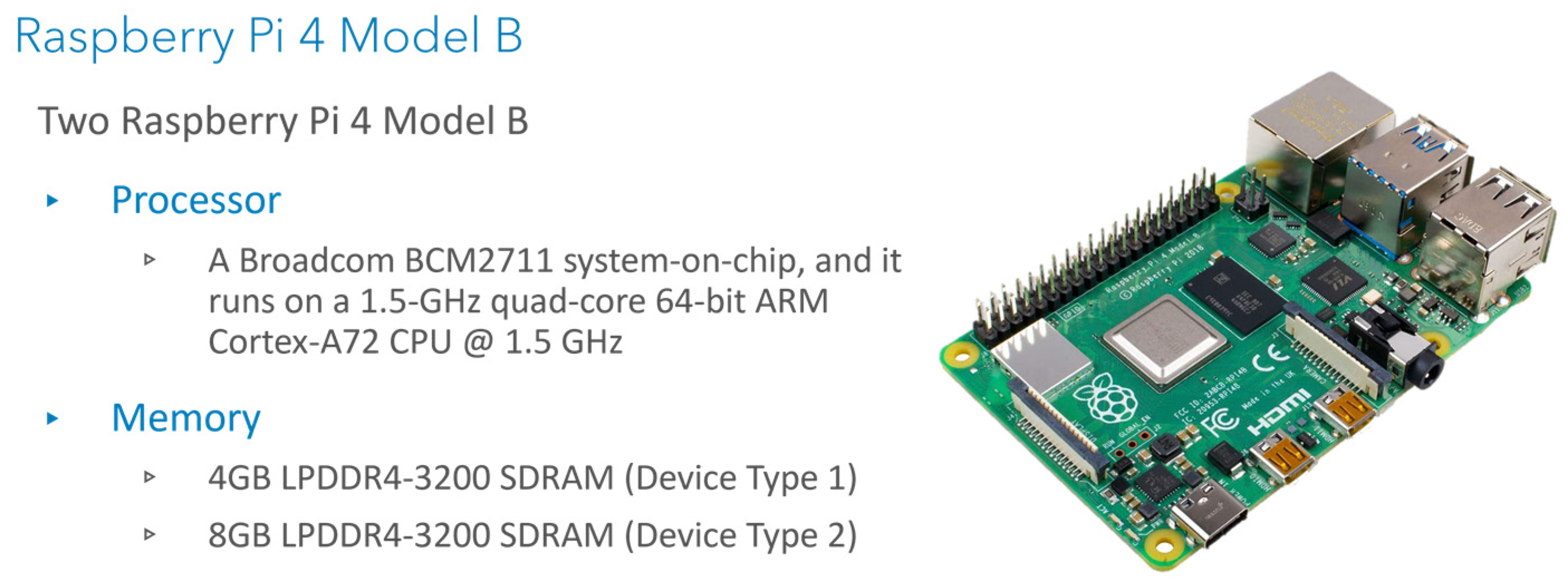
| 13 | Fog or Edge | Raspberry Pi Model B (8 GB) | 1.5 GHz Quad-core ARM Cortex-A72 8 GB Memory 2.4/5.0 GHz IEEE 802.11ac wireless | Idle: 2.7 W Working: 5.1 W | Wireless LAN Frequency Band: 2.4 GHz/5 GHz Data rate < 450 Mbps | Partially Configurable | A | |
| 14 | B | |||||||
| 15 | ALite | |||||||
| 16 | BLite | |||||||
| 17 | Fog or Edge | Raspberry Pi Model B (4 GB) | 1.5 GHz Quad-core ARM Cortex-A72 4 GB Memory 2.4/5.0 GHz IEEE 802.11ac wireless | Idle: 2.7 W Working: 5.1 W | Wireless LAN Frequency Band: 2.4 GHz/5 GHz Data rate < 450 Mbps | Partially Configurable | ALite | |
| 18 | BLite | |||||||
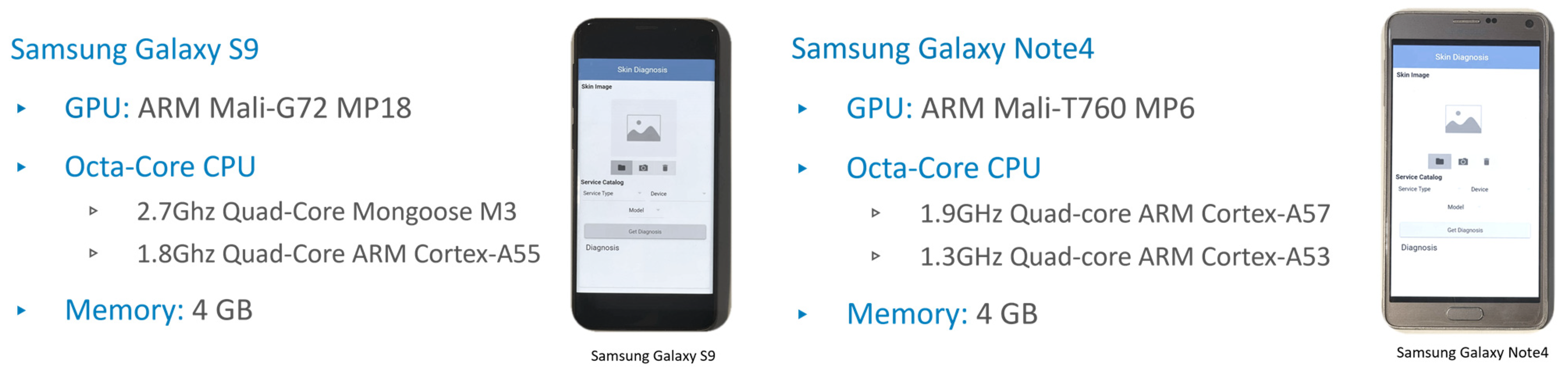
| 19 | Mobile Local Service | Edge | Samsung Galaxy S9 | GPU: ARM Mali-G72 MP18 Octa-Core, 2 CPUs: 2.7 Ghz Quad-Core Mongoose M3 1.8 Ghz Quad-Core ARM Cortex-A55 4 GB Memory | Idle: 1.09 W Working: 5.16 W | Wireless LAN Frequency Band: 2.4 GHz/5 GHz Data rate < 450 Mbps | Partially Configurable | ALite |
| 20 | BLite | |||||||
| 21 | Mobile Remote Service | Edge | Samsung Galaxy Note 4 | GPU: ARM Mali-T760 MP6 Octa-Core, 2 CPUs: 1.9 GHz Quad-core ARM Cortex-A57 1.3 GHz Quad-core ARM Cortex-A53 4 GB Memory | Idle: 1.4 W Working: 9.4 W | Wireless LAN Frequency Band: 2.4 GHz/5 GHz Data rate < 450 Mbps | Partially Configurable | ALite |
| 22 | BLite |
| Acronym | Definition | |
|---|---|---|
| 1 | CloudA | Model A (Executed on Cloud) |
| 2 | CloudB | Model B (Executed on Cloud) |
| 3 | CouldALite | Model ALite (Executed on Cloud) |
| 4 | CloudBLite | Model BLite (Executed on Cloud) |
| 5 | FogA | Model A (Executed on Fog—HP Laptop) |
| 6 | FogB | Model B (Executed on Fog—HP Laptop) |
| 7 | FogALite | Model ALite (Executed on Fog—HP Laptop) |
| 8 | FogBLite | Model BLite (Executed on Fog—HP Laptop) |
| 9 | JetsonA | Model A (Executed on Jetson) |
| 10 | JetsonB | Model B (Executed on Jetson) |
| 11 | JetsonALite | Model ALite (Executed on Jetson) |
| 12 | JetsonBLite | Model BLite (Executed on Jetson) |
| 13 | Rasp8A | Model A (Executed on Raspberry pi 8 GB) |
| 14 | Rasp8B | Model B (Executed on Raspberry pi 8 GB) |
| 15 | Rasp8ALite | Model ALite (Executed on Raspberry pi 8 GB) |
| 16 | Rasp8BLite | Model BLite (Executed on Raspberry pi 8 GB) |
| 17 | Rasp4ALite | Model ALite (Executed on Raspberry pi 4 GB) |
| 18 | Rasp4BLite | Model BLite (Executed on Raspberry pi 4 GB) |
| 19 | MobileLALite | Model ALite (Executed on Local Mobile—Galaxy S9) |
| 20 | MobileLBLite | Model BLite (Executed on Local Mobile—Galaxy S9) |
| 21 | MobileRALite | Model ALite (Executed on Remote Mobile—Galaxy Note 4) |
| 22 | MobileRBLite | Model BLite (Executed on Remote Mobile—Galaxy Note 4) |
| Class | Diagnostic Categories | Code | Images | Sample |
|---|---|---|---|---|
| 0 | Actinic Keratoses and Intraepithelial Carcinoma/Bowen’s Disease | akiec | 327 |  |
| 1 | Basal Cell Carcinoma | bcc | 514 |  |
| 2 | Benign Keratosis-Like Lesions (Solar Lentigines/Seborrheic Keratoses and Lichen-Planus-Like Keratoses) | bkl | 1099 |  |
| 3 | Dermatofibroma | df | 115 |  |
| 4 | Melanoma | mel | 1113 |  |
| 5 | Melanocytic Nevi | nv | 6705 |  |
| 6 | Vascular Lesions (Angiomas, Angiokeratomas, Pyogenic Granulomas, and Hemorrhage) | vasc | 142 |  |
| Total Number of Images | 10,015 | |||
| Model | Layers | Total Parameters | TensorFlow | TensorFlow Lite | Size Ratio | ||||
|---|---|---|---|---|---|---|---|---|---|
| RAM (MB) | Training (%) | Validation (%) | Testing (%) | RAM (MB) | Testing (%) | ||||
| A | 55 | 23,057,255 | 264 | 95.64 | 83.23 | 82.38 | 87.8 | 82.38 | 3.01 |
| B | 19 | 3,833,367 | 43.9 | 79.05 | 78.28 | 77.33 | 14.6 | 77.33 | |
| Variable | Definition | Unit | Example |
|---|---|---|---|
| Date | Date of the request | Date | 16/02/2021 |
| Day | Day of the week | Date | Tuesday |
| Hour | Time of the request | Time | 06:15:49.333 |
| ImageName | Image name from the dataset | String | ISIC_0033458 |
| ModelVersion | Model used for classification (A = 1, B = 2, ALite = 3, BLite = 4) | Number | 1 |
| DeviceName | The name of the device: Cloud, Laptop, Jetson, Rasp8, Rasp4, S9, Note 4 | String | Cloud |
| RequestSize | The packet size of the request message | Bytes | 171,316 |
| RequestSentTimestamp | The timestamp when the request is sent by the user | Milliseconds | 1,613,445,211,566 |
| RequestReceiveTimestamp | The timestamp when the request is received at the service | Milliseconds | 1,613,445,342,877 |
| ServiceProcessTime | The service processing time (inference or compute) | Milliseconds | 6334 |
| ResponseSentTimestamp | The timestamp when the response is sent from the service | Milliseconds | 1,613,445,349,211 |
| ResponseReceiveTimestamp | The timestamp when the response is received at the user device | Milliseconds | 1,613,445,349,325 |
| ResponseTime | The total time taken to obtain a response, from the moment the request had been made | Milliseconds | 137,759 |
| ResponseSize | The packet size of the response message | Bytes | 112 |
| Result | Diagnosis results as a probability of each class of the diseases (7 values for 7 classes separated by commas) | List of floats | [4.025427 × 10⁻⁷, 1.1340192 × 10⁻⁷, 4.8968374 × 10⁻⁸, 6.5097774 × 10⁻⁶, 3.8256036 × 10⁻⁷, 0.00020890325, 0.9997837] |
Publisher’s Note: MDPI stays neutral with regard to jurisdictional claims in published maps and institutional affiliations. |
© 2022 by the authors. Licensee MDPI, Basel, Switzerland. This article is an open access article distributed under the terms and conditions of the Creative Commons Attribution (CC BY) license (https://creativecommons.org/licenses/by/4.0/).
Share and Cite
Janbi, N.; Mehmood, R.; Katib, I.; Albeshri, A.; Corchado, J.M.; Yigitcanlar, T. Imtidad: A Reference Architecture and a Case Study on Developing Distributed AI Services for Skin Disease Diagnosis over Cloud, Fog and Edge. Sensors 2022, 22, 1854. https://doi.org/10.3390/s22051854
Janbi N, Mehmood R, Katib I, Albeshri A, Corchado JM, Yigitcanlar T. Imtidad: A Reference Architecture and a Case Study on Developing Distributed AI Services for Skin Disease Diagnosis over Cloud, Fog and Edge. Sensors. 2022; 22(5):1854. https://doi.org/10.3390/s22051854
Chicago/Turabian StyleJanbi, Nourah, Rashid Mehmood, Iyad Katib, Aiiad Albeshri, Juan M. Corchado, and Tan Yigitcanlar. 2022. "Imtidad: A Reference Architecture and a Case Study on Developing Distributed AI Services for Skin Disease Diagnosis over Cloud, Fog and Edge" Sensors 22, no. 5: 1854. https://doi.org/10.3390/s22051854