
Selecting Some Variables to Update-Based Algorithm for Solving Optimization Problems


Abstract
:1. Introduction
- A new stochastic-based approach called Selecting Some Variables to Update-Based Algorithm (SSVUBA) used in optimization issues is introduced.
- The fundamental idea behind the proposed method is to change the number of selected variables to update the algorithm population throughout iterations, as well as to use more information from diverse members of the population to prevent the algorithm from relying on one or several specific members.
- SSVUBA theory and steps are described and its mathematical model is presented.
- On a set of fifty-three standard objective functions of various unimodal, multimodal types, and CEC 2017, SSVUBA’s capacity to optimize is examined.
- The proposed algorithm is implemented in four engineering design problems to analyze SSVUBA’s ability to solve real-world applications,
- SSVUBA’s performance is compared to the performance of eight well-known algorithms to better understand its potential to optimize.
2. Background
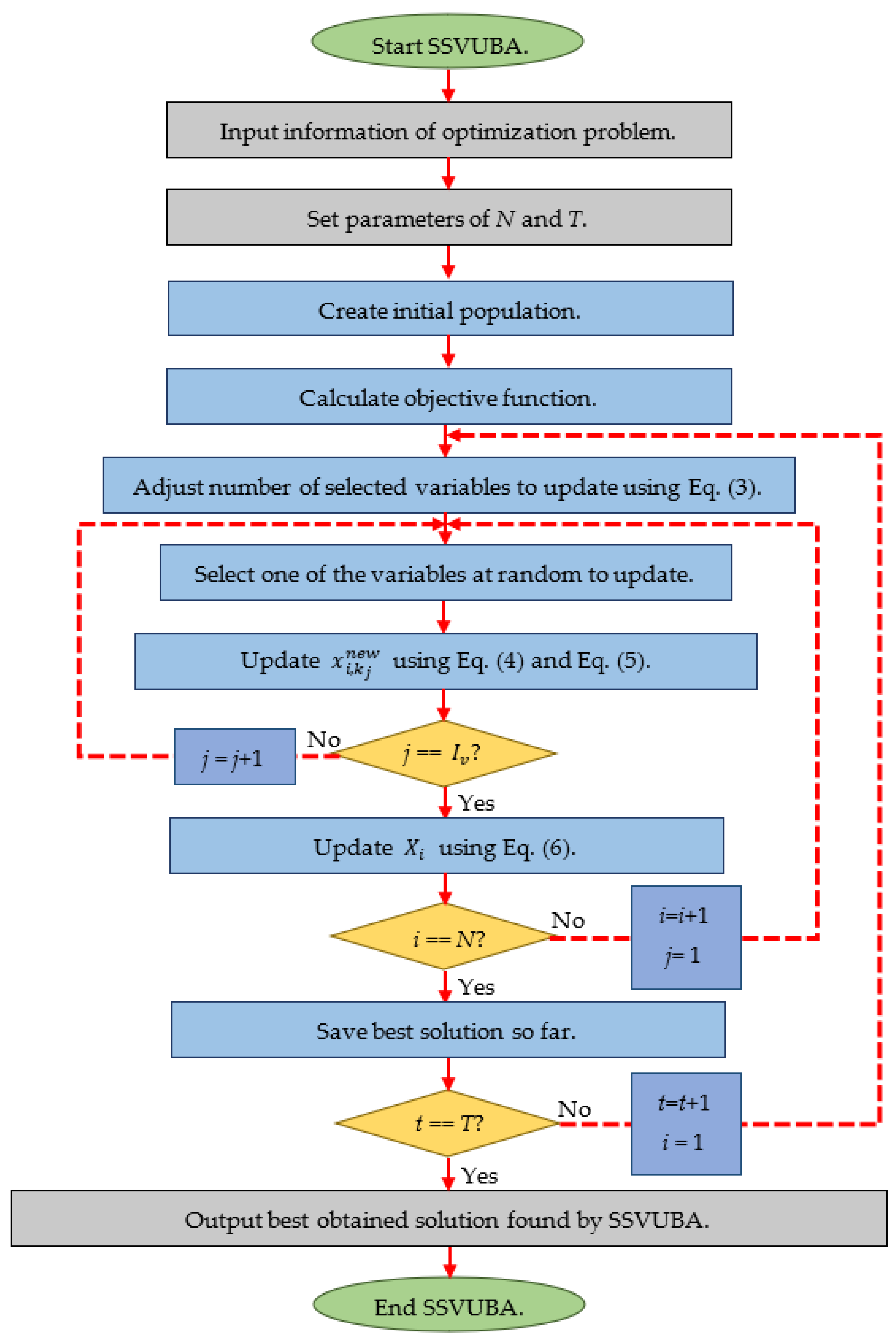
3. Selecting Some Variables to Update-Based Algorithm (SSVUBA)
3.1. Mathmatical Model of SSVUBA
3.2. Repetition Process of SSVUBA
3.3. Computational Complexity of SSVUBA
3.3.1. Time Complexity
3.3.2. Space Complexity
| Algorithm 1. Pseudo-code of SSVUBA | ||||||
| Start SSVUBA. | ||||||
| 1. | Input the optimization problem information: Decision variables, constraints, and objective function | |||||
| 2. | Set the T and N parameters. | |||||
| 3. | For t = 1:T | |||||
| 4. | ||||||
| 5. | For i = 1:N | |||||
| 6. | For j = 1: | |||||
| 7. | Select a population member randomly to guide the ith population member. , is the Sth row of the population matrix. | |||||
| 8. | Select one of the variables at random to update. . | |||||
| 9. | ||||||
| 10. | If | |||||
| 11. | ||||||
| 12. | else | |||||
| 13. | ||||||
| 14. | end | |||||
| 15. | end | |||||
| 16. | ||||||
| 17. | If | |||||
| 18. | ||||||
| 19. | else | |||||
| 20. | ||||||
| 21. | end | |||||
| 22. | end | |||||
| 23. | Save the best solution so far. | |||||
| 24. | end | |||||
| 25. | Output the best obtained solution. | |||||
| End SSVUBA. | ||||||
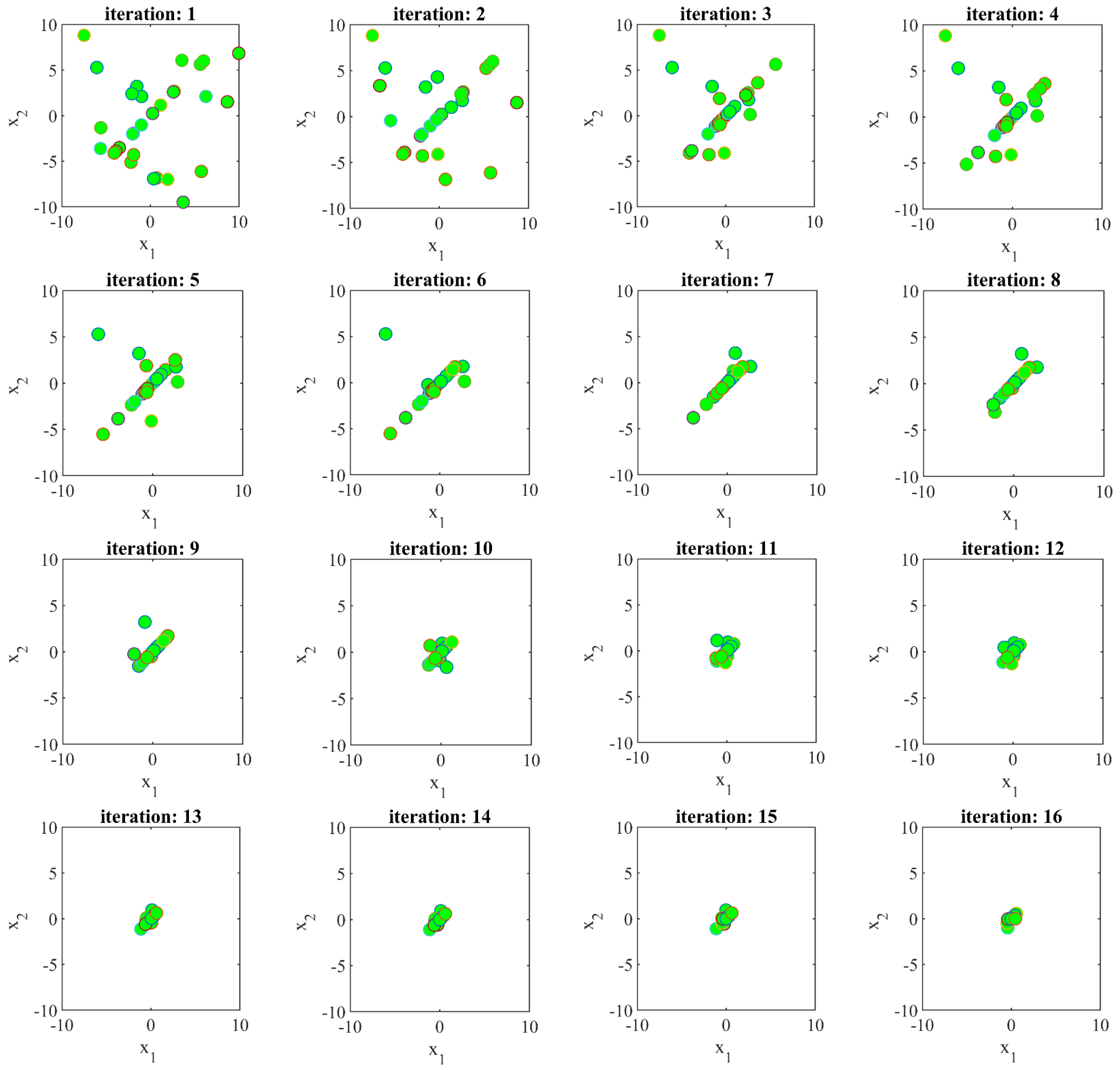
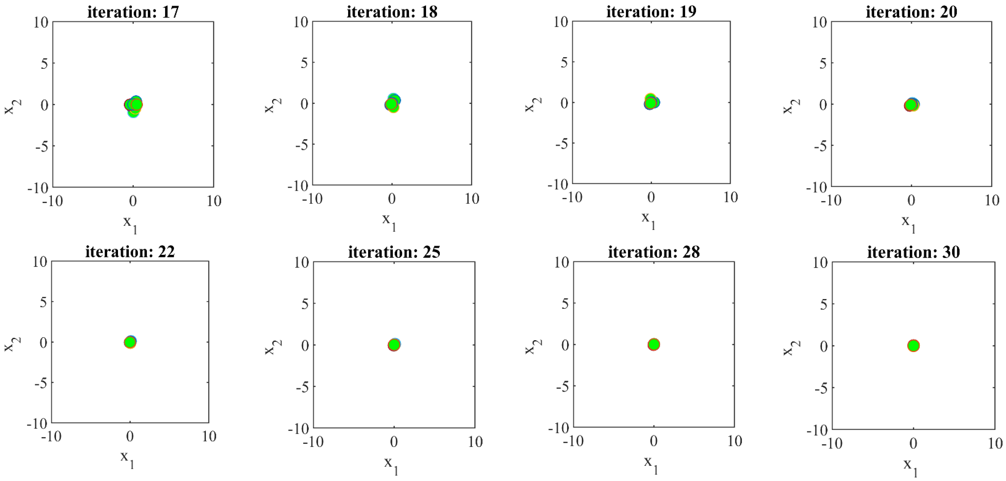
3.4. Visualization of the Movement of Population Members towards the Solution
4. Simulation Studies and Results
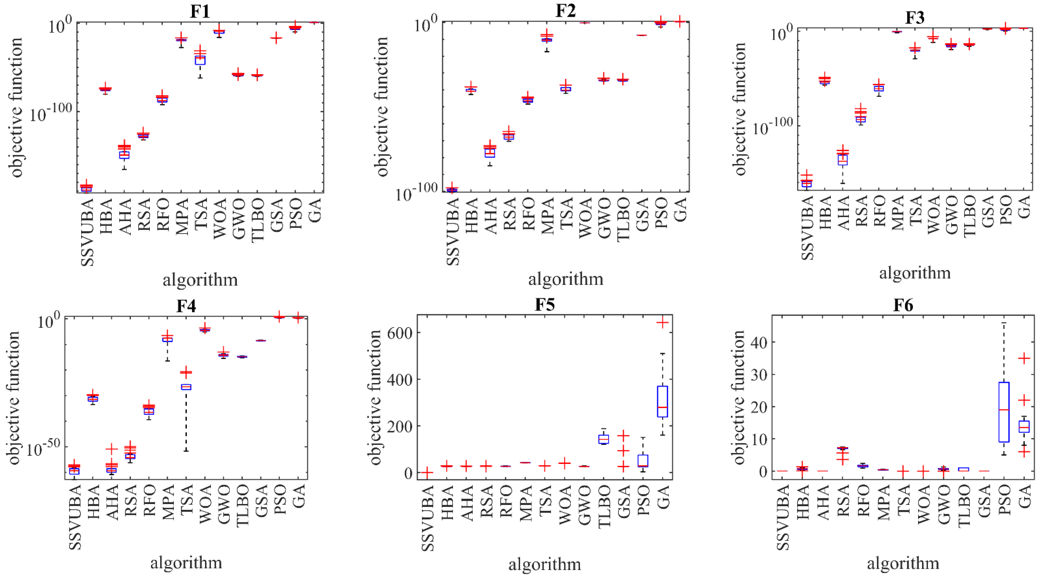
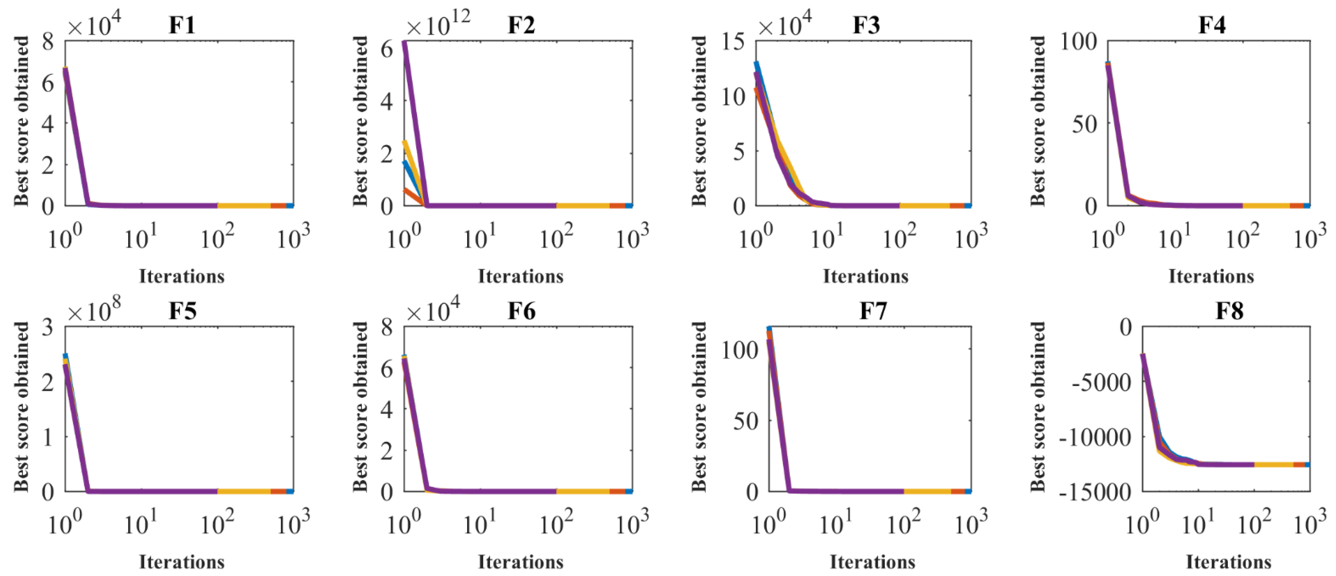
4.1. Assessment of F1 to F7 Unimodal Functions
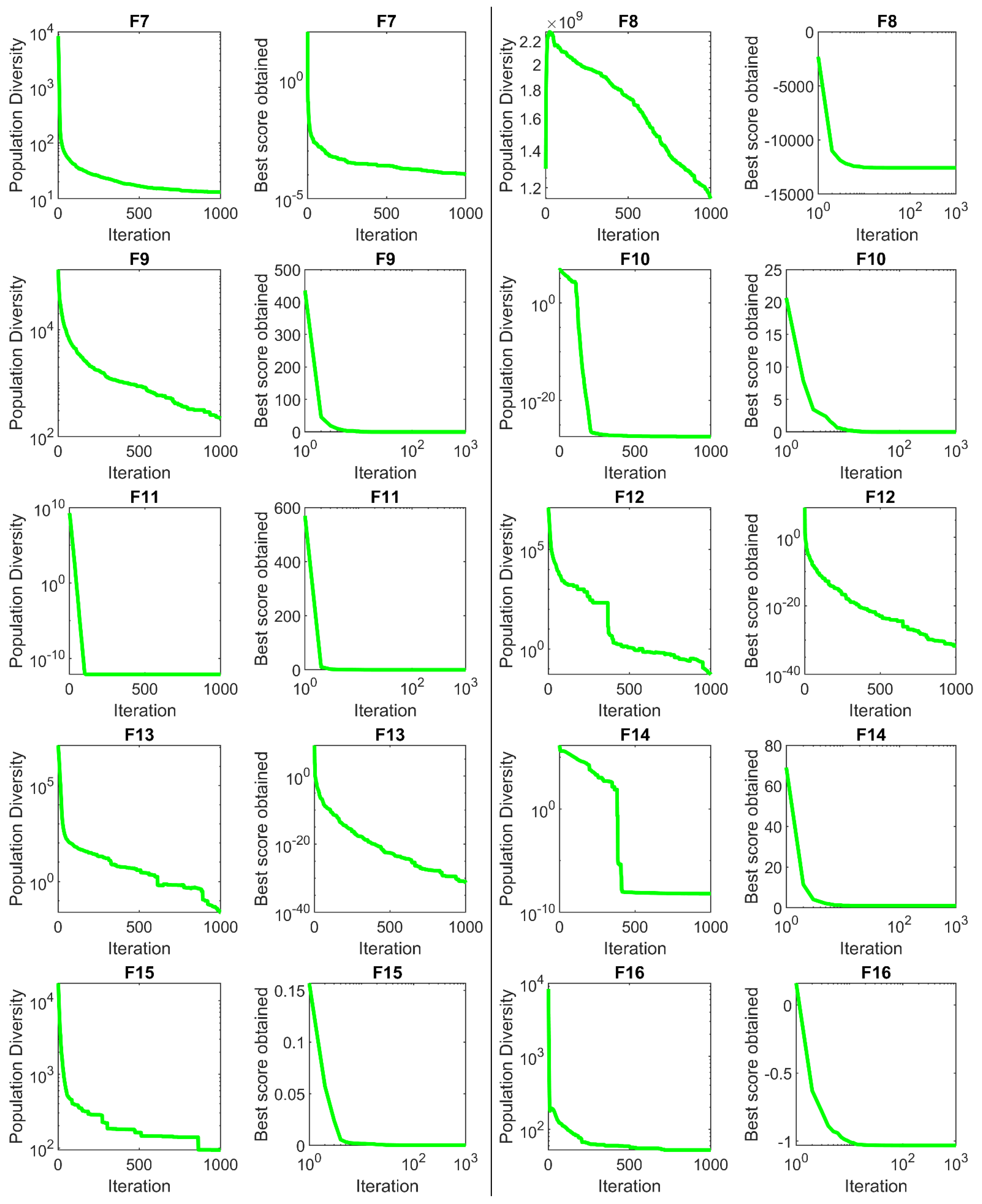
4.2. Assessment of F8 to F13 High-Dimensional Multimodal Functions
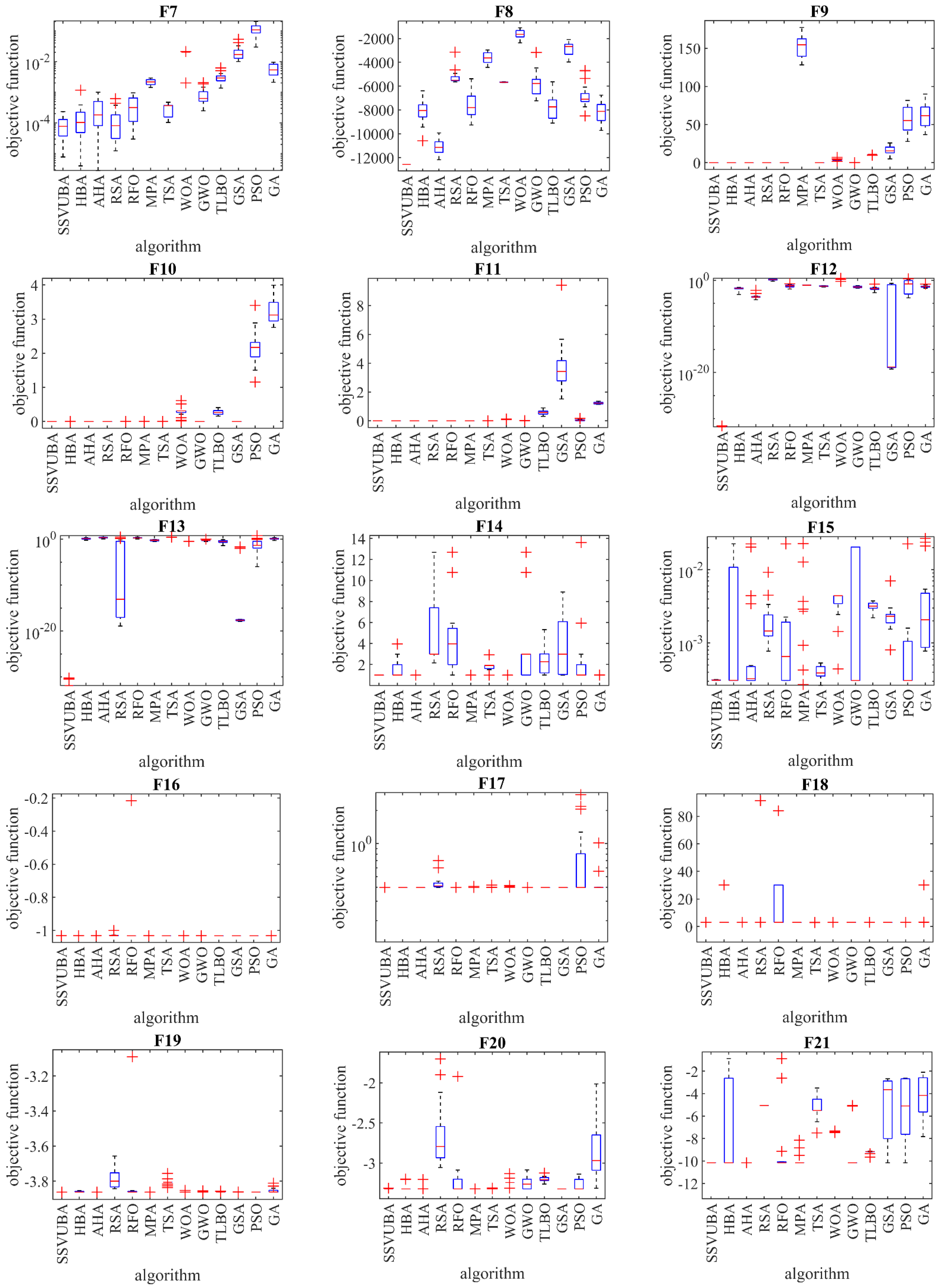
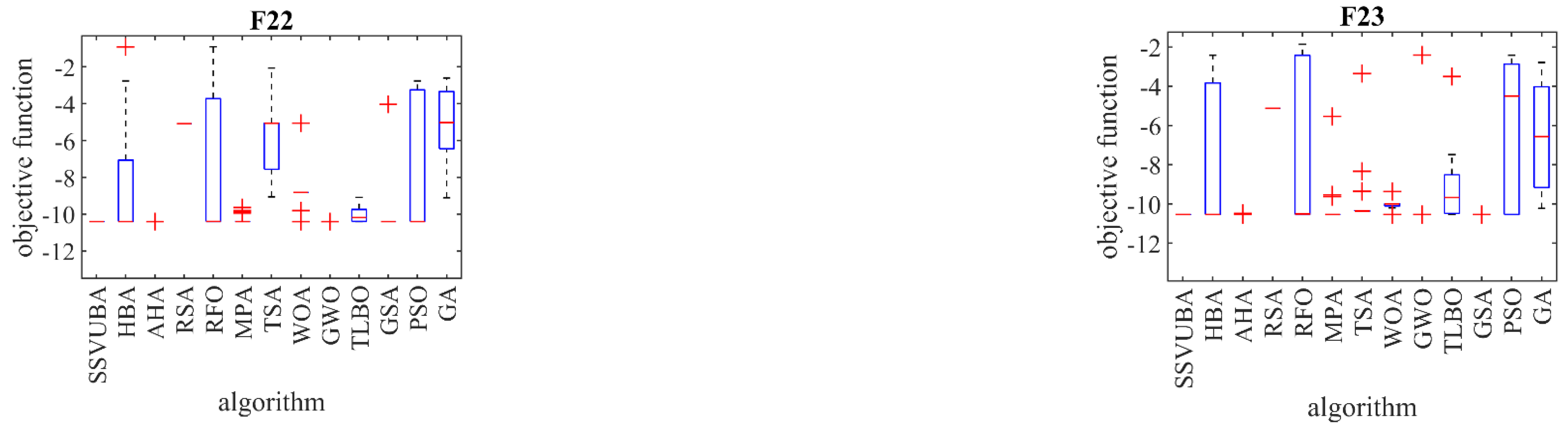
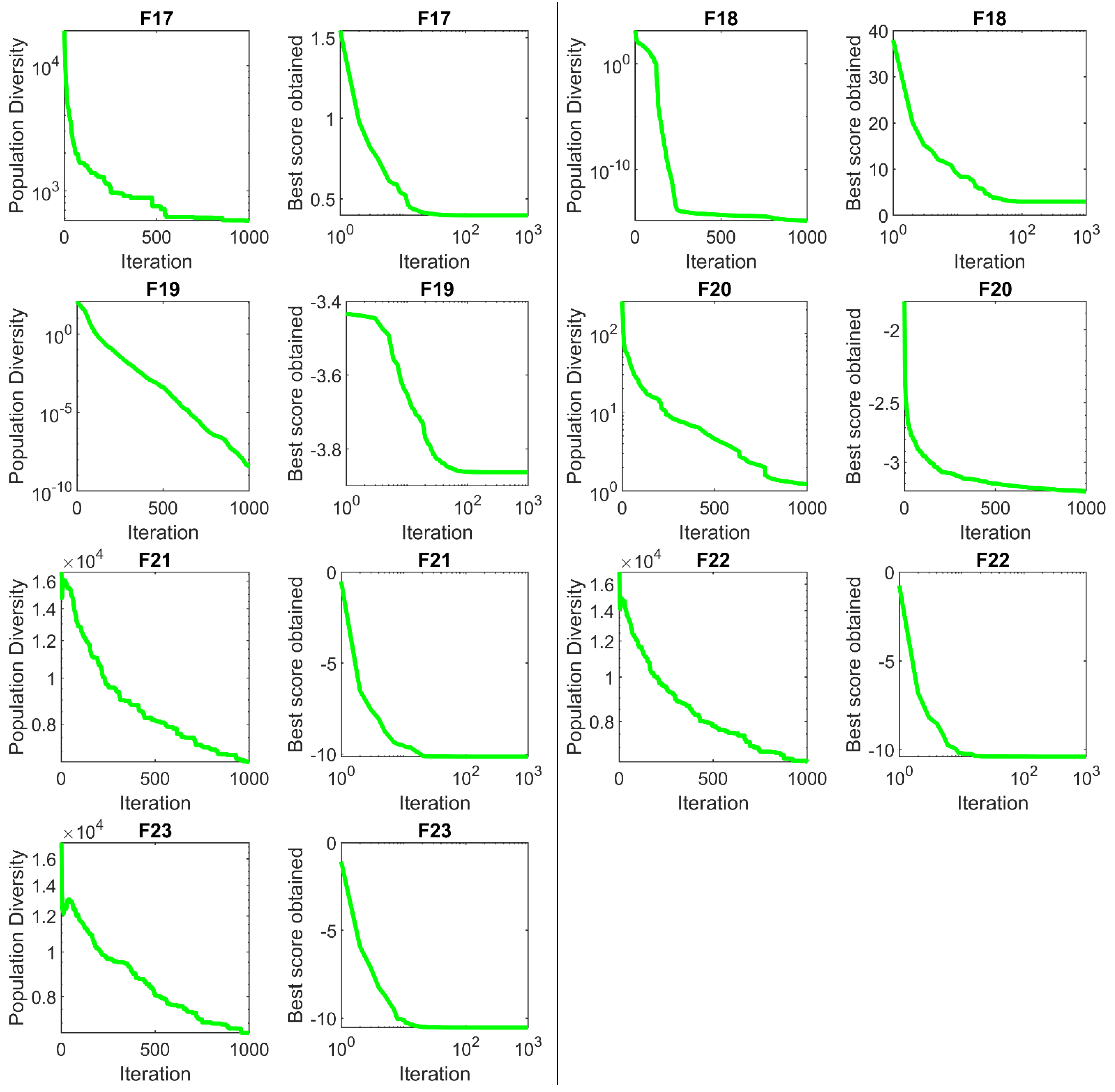
4.3. Assessment of F14 to F23 Fixed-Dimensional Multimodal Functions
4.4. Statistical Analysis
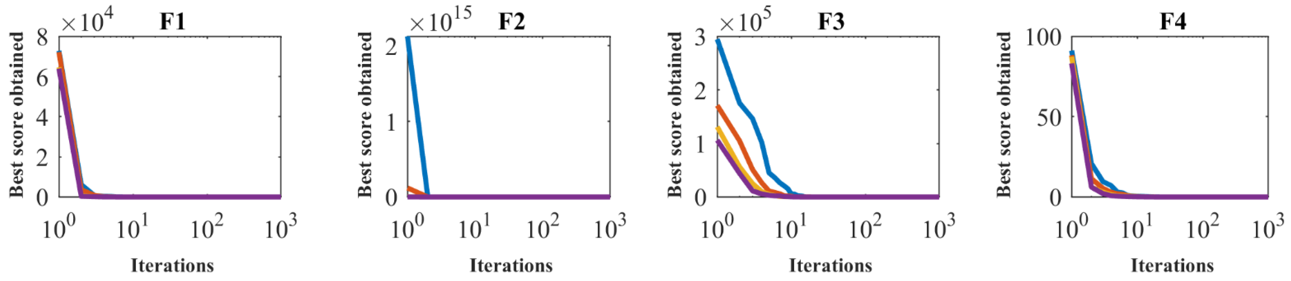
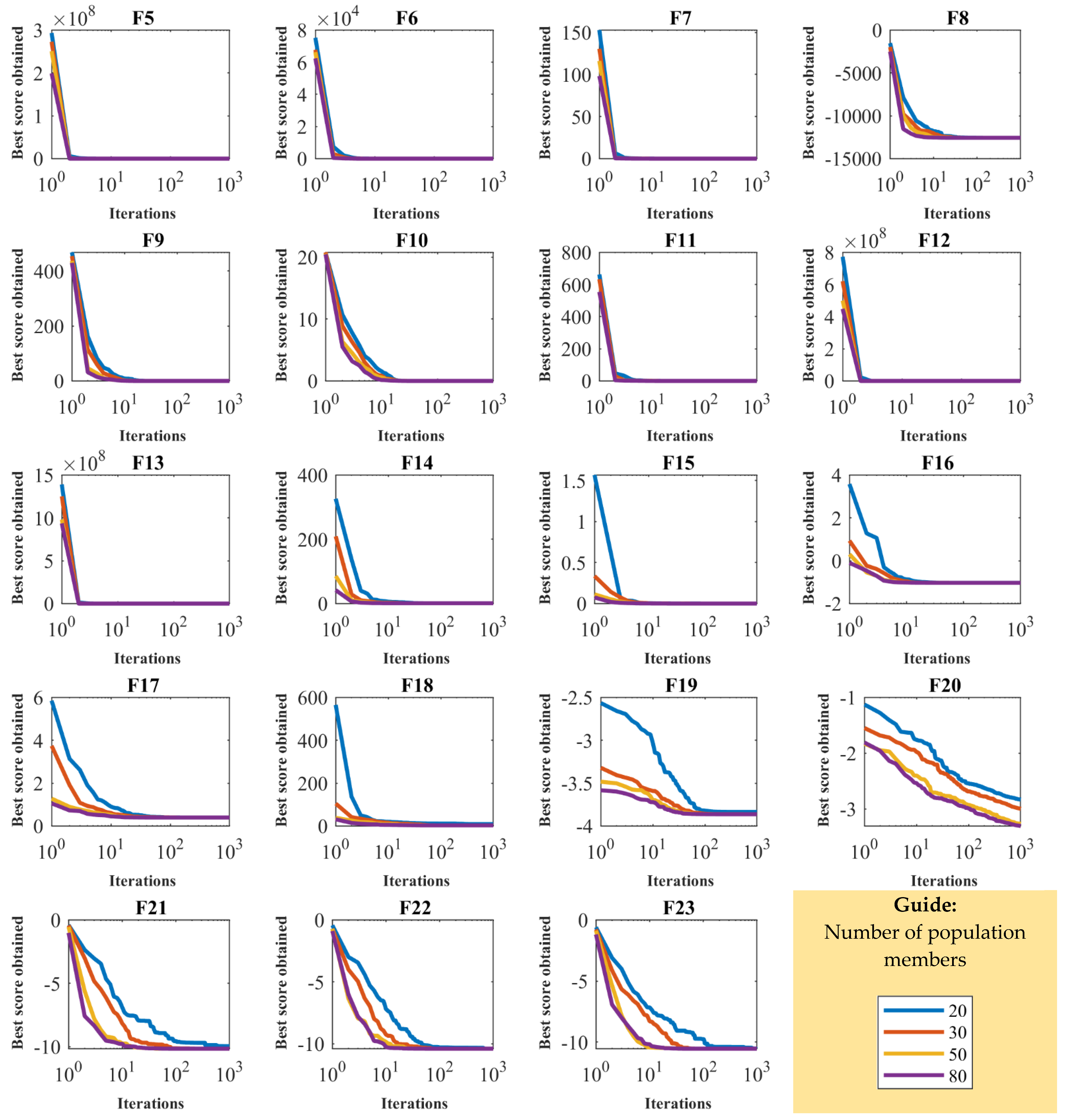
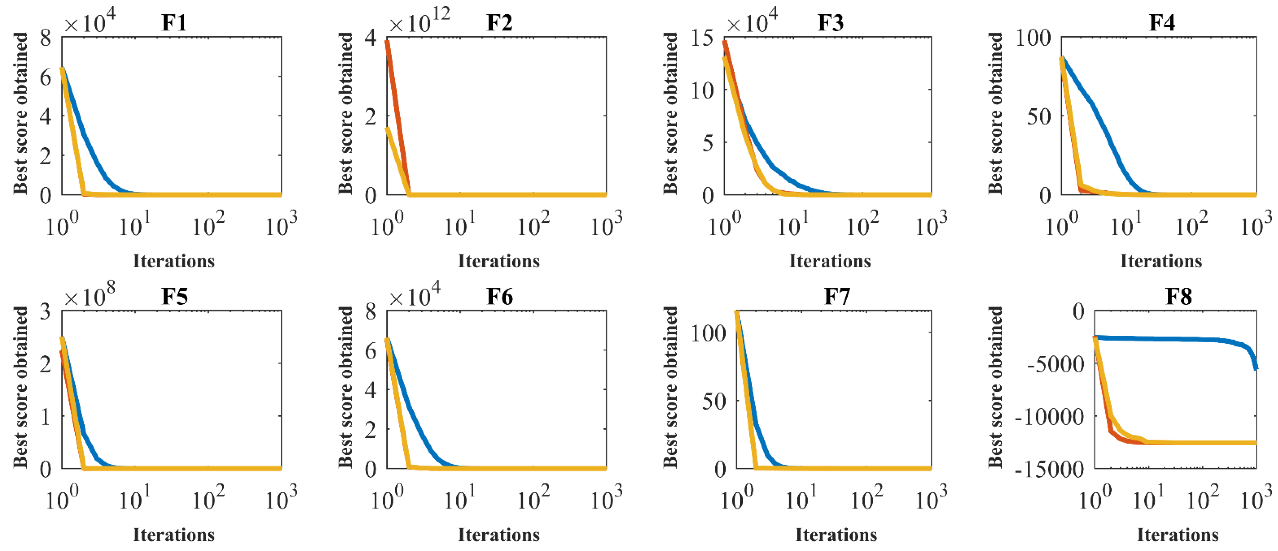
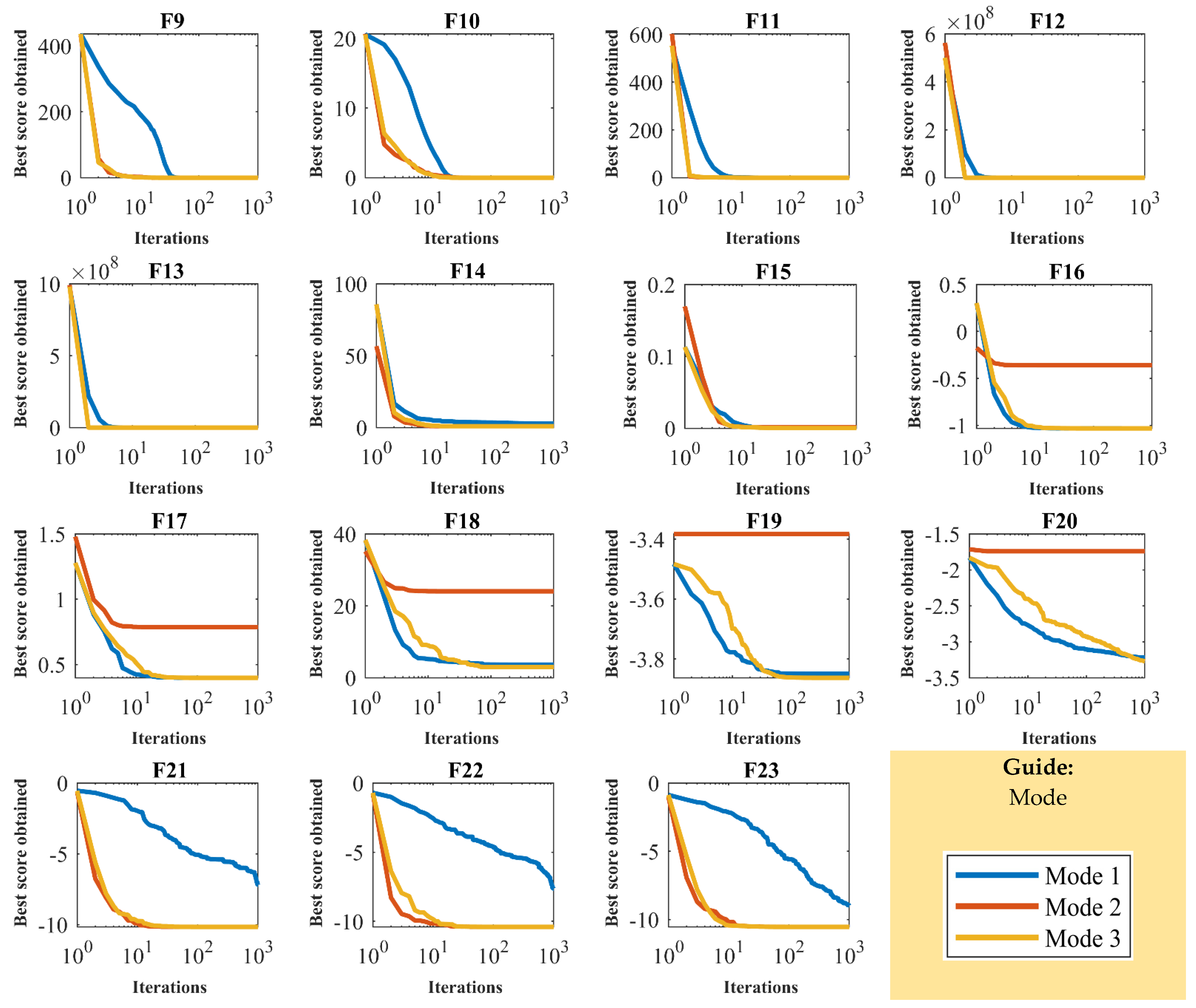
4.5. Sensitivity Analysis
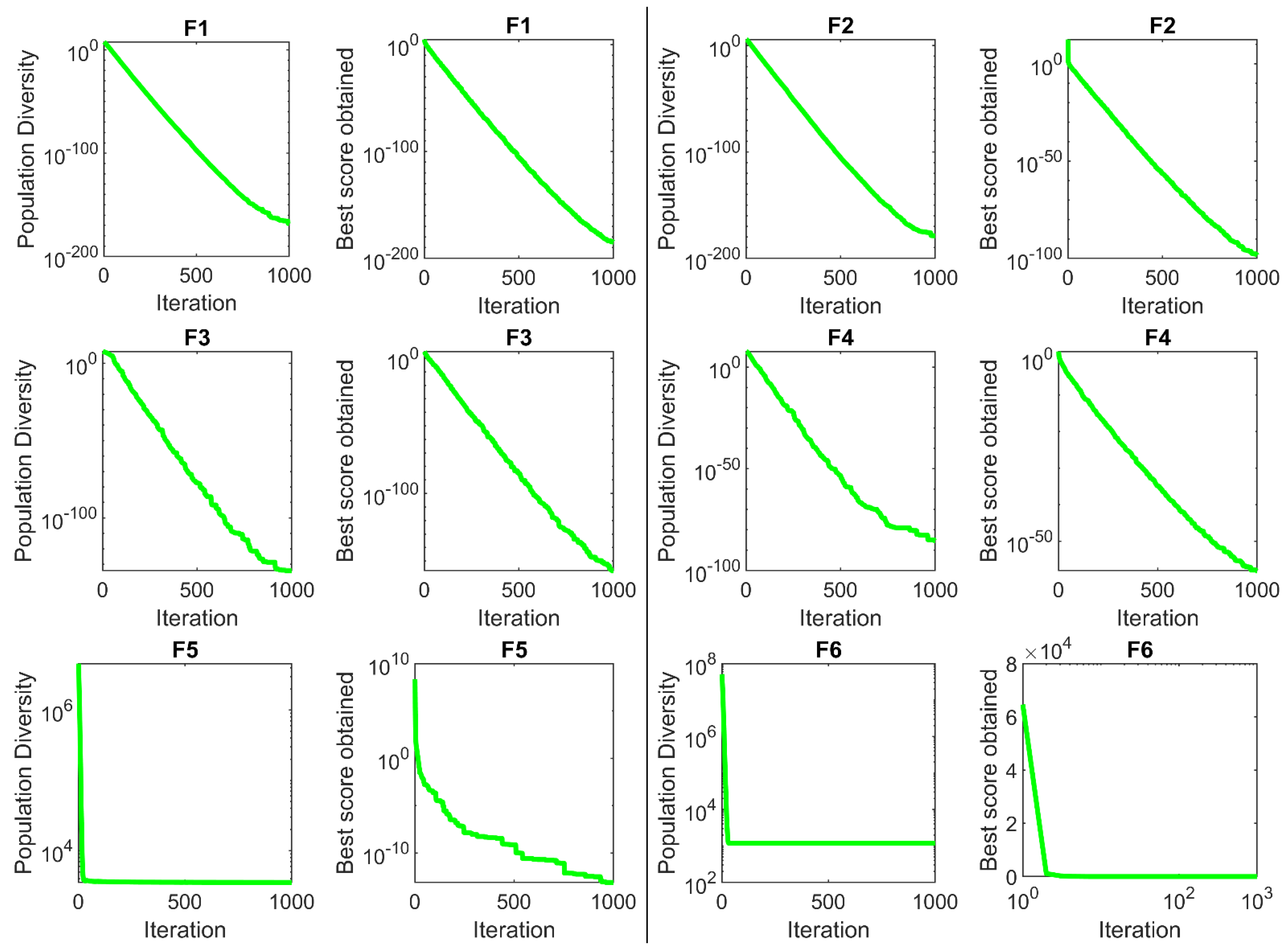
4.6. Population Diversity Analysis
4.7. Evaluation of the CEC 2017 Test Functions
5. Discussion
6. SSVUBA for Engineering Design Applications
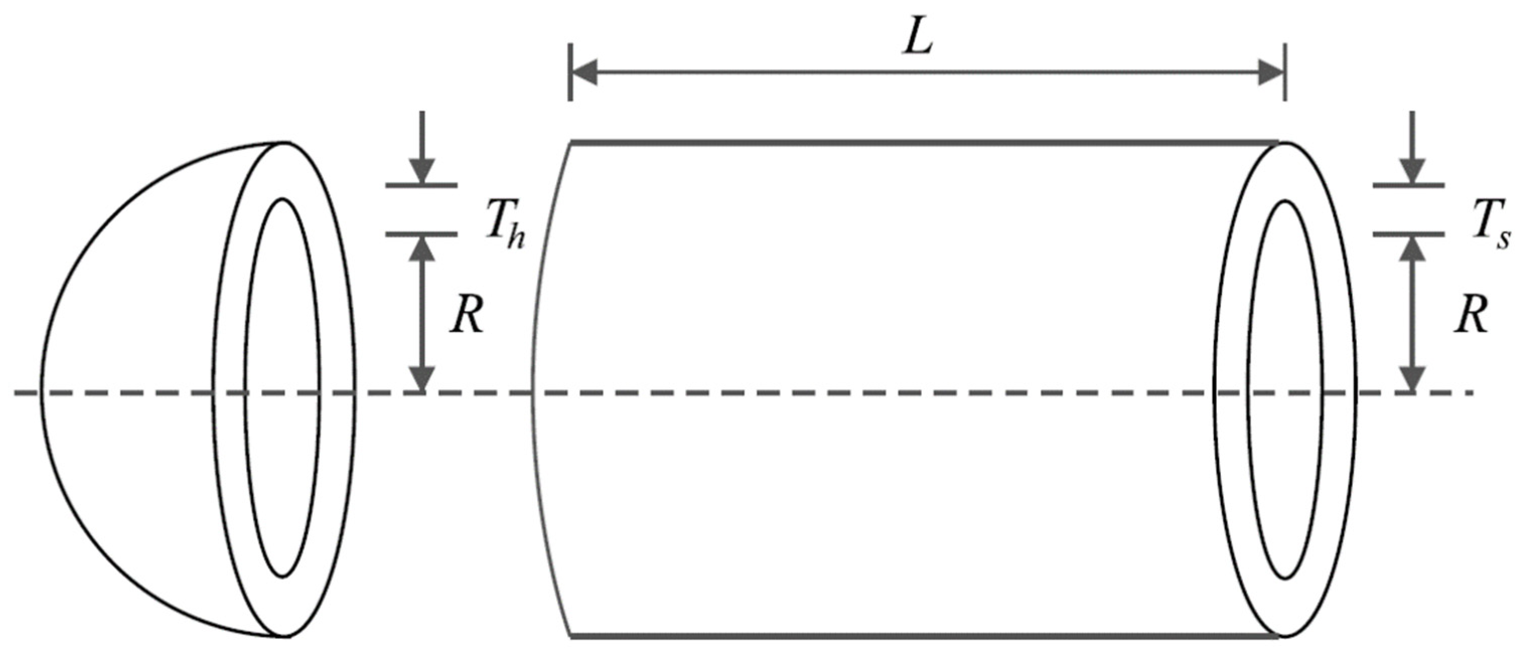
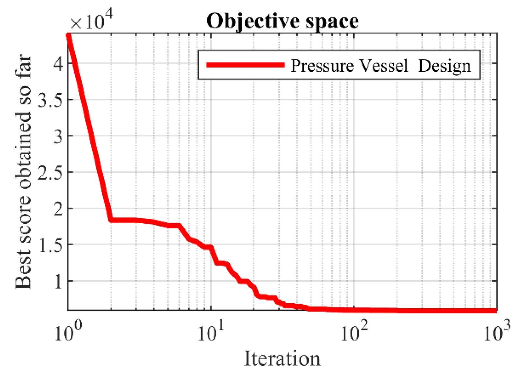
6.1. Pressure Vessel Design Problem
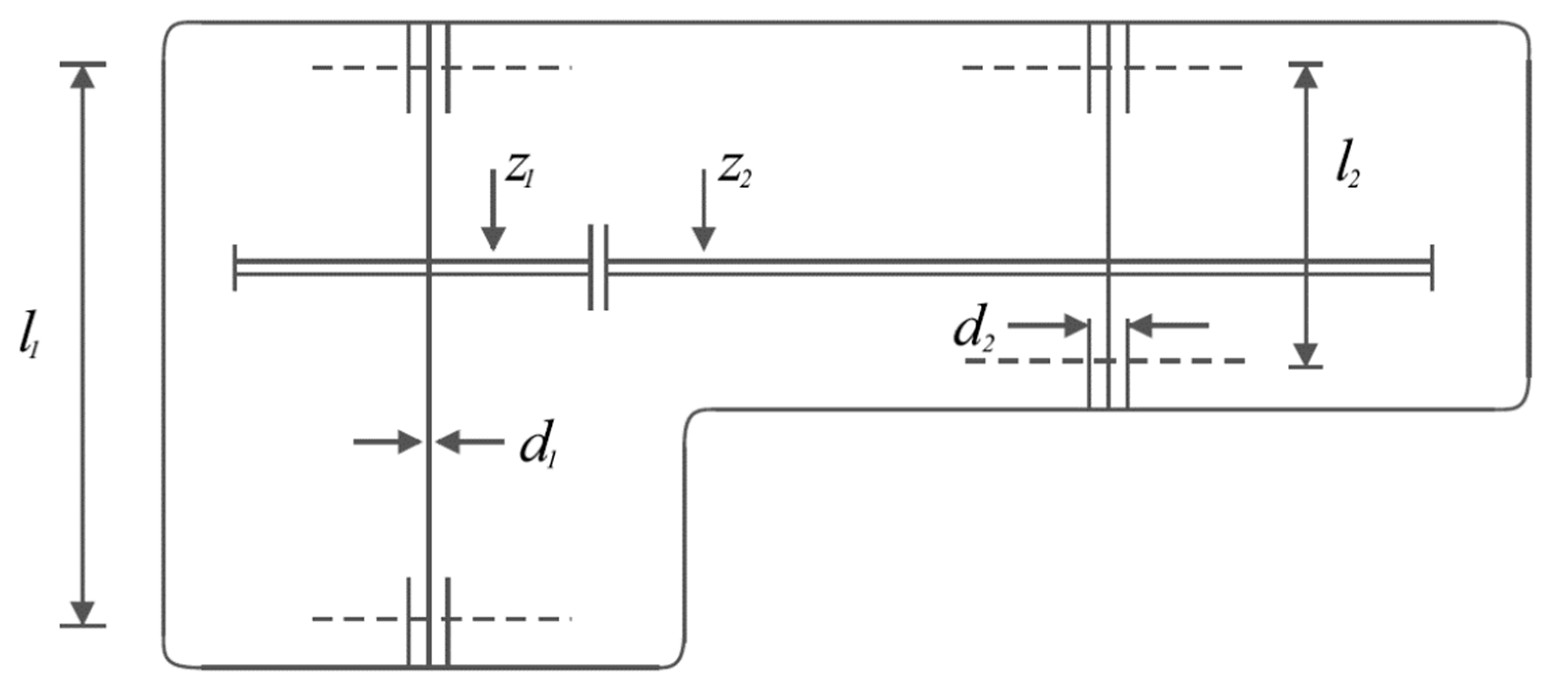
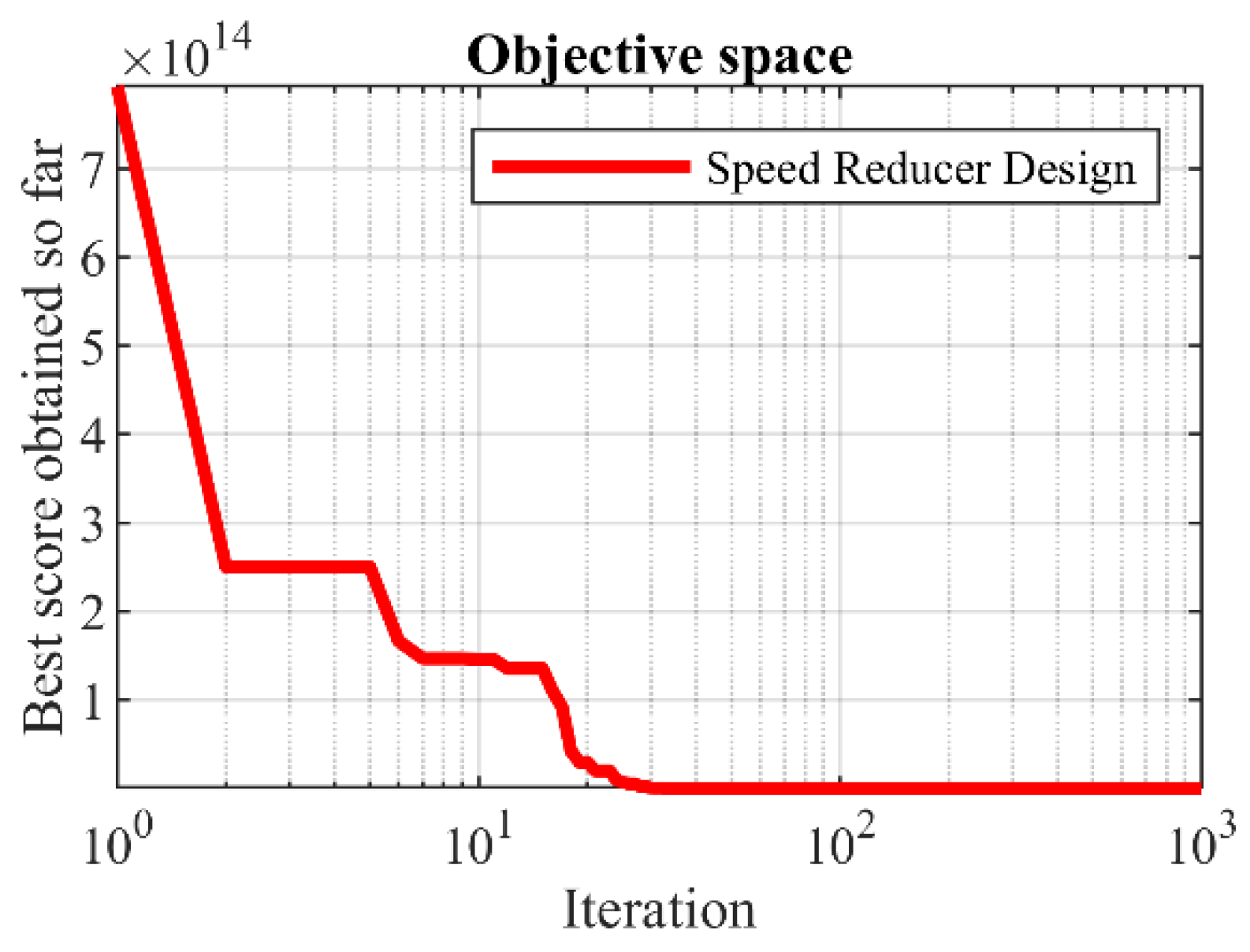
6.2. Speed Reducer Design Problem
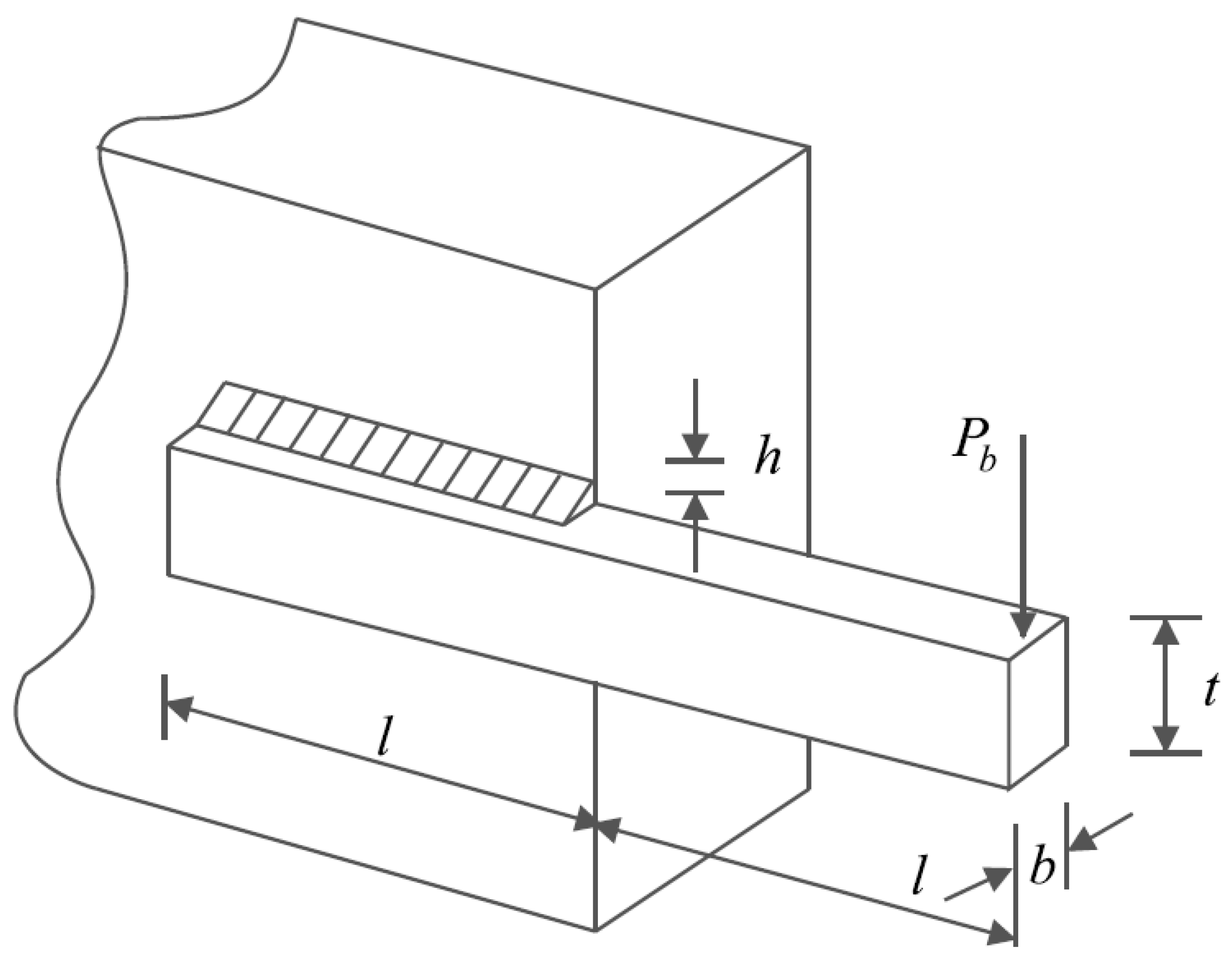
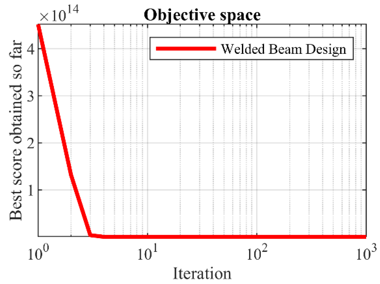
6.3. Welded Beam Design
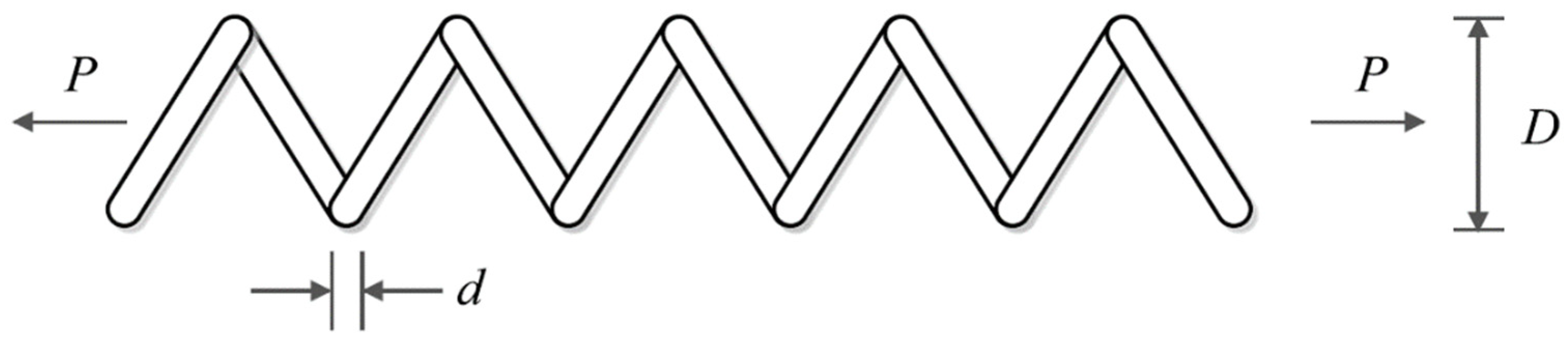
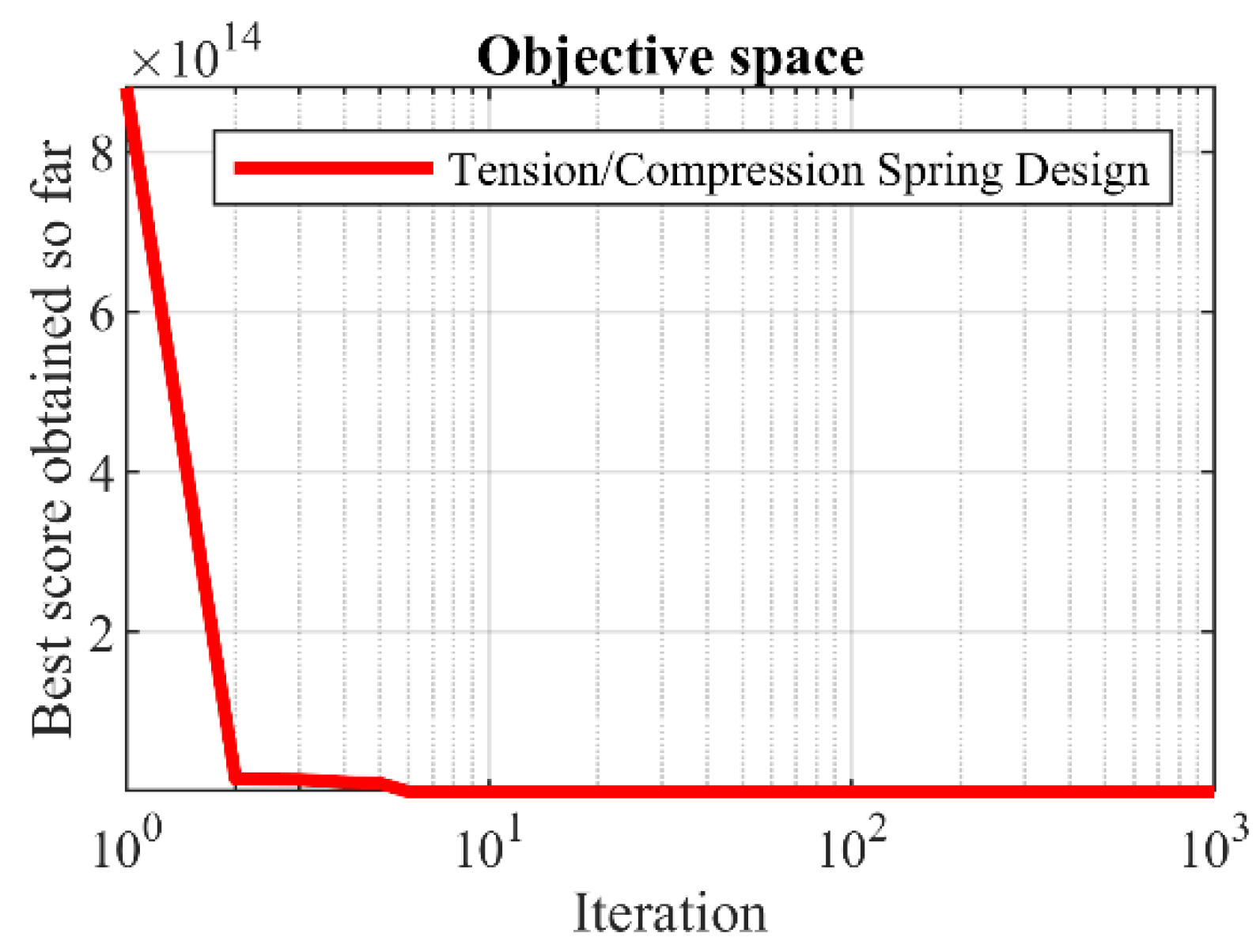
6.4. Tension/Compression Spring Design Problem
6.5. The SSVUBA’s Applicability in Sensor Networks and Image Processing
7. Conclusions and Future Works
Author Contributions
Funding
Institutional Review Board Statement
Informed Consent Statement
Data Availability Statement
Acknowledgments
Conflicts of Interest
Appendix A

| Objective Function | Range | Dimensions | |
|---|---|---|---|
| 30 | 0 | ||
| 30 | 0 | ||
| 30 | 0 | ||
| 30 | 0 | ||
| 30 | 0 | ||
| 30 | 0 | ||
| 30 | 0 |
| Objective Function | Range | Dimensions | |
|---|---|---|---|
| 30 | −12,569 | ||
| 30 | 0 | ||
| 30 | 0 | ||
| 30 | 0 | ||
| 30 | 0 | ||
| 30 | 0 |
| Objective Function | Range | Dimensions | |
|---|---|---|---|
| 2 | 0.998 | ||
| 4 | 0.00030 | ||
| 2 | −1.0316 | ||
| [−5, 10] [0, 15] | 2 | 0.398 | |
| 2 | 3 | ||
| 3 | −3.86 | ||
| 6 | −3.22 | ||
| 4 | −10.1532 | ||
| 4 | −10.4029 | ||
| 4 | −10.5364 |
| Functions | |||
|---|---|---|---|
| Unimodal functions | C1 | Shifted and Rotated Bent Cigar Function | 100 |
| C2 | Shifted and Rotated Sum of Different Power Function | 200 | |
| C3 | Shifted and Rotated Zakharov Function | 300 | |
| Simple multimodal functions | C4 | Shifted and Rotated Rosenbrock Function | 400 |
| C5 | Shifted and Rotated Rastrigin Function | 500 | |
| C6 | Shifted and Rotated Expanded Scaffer Function | 600 | |
| C7 | Shifted and Rotated Lunacek Bi_Rastrigin Function | 700 | |
| C8 | Shifted and Rotated Non-Continuous Rastrigin Function | 800 | |
| C9 | Shifted and Rotated Levy Function | 900 | |
| C10 | Shifted and Rotated Schwefel Function | 1000 | |
| Hybrid functions | C11 | Hybrid Function 1 (N = 3) | 1100 |
| C12 | Hybrid Function 2 (N = 3) | 1200 | |
| C13 | Hybrid Function 3 (N = 3) | 1300 | |
| C14 | Hybrid Function 4 (N = 4) | 1400 | |
| C15 | Hybrid Function 5 (N = 4) | 1500 | |
| C16 | Hybrid Function 6 (N = 4) | 1600 | |
| C17 | Hybrid Function 6 (N = 5) | 1700 | |
| C18 | Hybrid Function 6 (N = 5) | 1800 | |
| C19 | Hybrid Function 6 (N = 5) | 1900 | |
| C20 | Hybrid Function 6 (N = 6) | 2000 | |
| Composition functions | C21 | Composition Function 1 (N = 3) | 2100 |
| C22 | Composition Function 2 (N = 3) | 2200 | |
| C23 | Composition Function 3 (N = 4) | 2300 | |
| C24 | Composition Function 4 (N = 4) | 2400 | |
| C25 | Composition Function 5 (N = 5) | 2500 | |
| C26 | Composition Function 6 (N = 5) | 2600 | |
| C27 | Composition Function 7 (N = 6) | 2700 | |
| C28 | Composition Function 8 (N = 6) | 2800 | |
| C29 | Composition Function 9 (N = 3) | 2900 | |
| C30 | Composition Function 10 (N = 3) | 3000 |
References
- Dhiman, G. SSC: A hybrid nature-inspired meta-heuristic optimization algorithm for engineering applications. Knowl.-Based Syst. 2021, 222, 106926. [Google Scholar] [CrossRef]
- Fletcher, R. Practical Methods of Optimization; John Wiley & Sons: Hoboken, NJ, USA, 2013. [Google Scholar]
- Cavazzuti, M. Deterministic Optimization. In Optimization Methods: From Theory to Design Scientific and Technological Aspects in Mechanics; Springer: Berlin/Heidelberg, Germany, 2013; pp. 77–102. [Google Scholar]
- Dehghani, M.; Montazeri, Z.; Dehghani, A.; Samet, H.; Sotelo, C.; Sotelo, D.; Ehsanifar, A.; Malik, O.P.; Guerrero, J.M.; Dhiman, G. DM: Dehghani Method for modifying optimization algorithms. Appl. Sci. 2020, 10, 7683. [Google Scholar] [CrossRef]
- Iba, K. Reactive power optimization by genetic algorithm. IEEE Trans. Power Syst. 1994, 9, 685–692. [Google Scholar] [CrossRef]
- Banerjee, A.; De, S.K.; Majumder, K.; Das, V.; Giri, D.; Shaw, R.N.; Ghosh, A. Construction of effective wireless sensor network for smart communication using modified ant colony optimization technique. In Advanced Computing and Intelligent Technologies; Springer: Berlin/Heidelberg, Germany, 2022; pp. 269–278. [Google Scholar]
- Zhang, X.; Dahu, W. Application of artificial intelligence algorithms in image processing. J. Vis. Commun. Image Represent. 2019, 61, 42–49. [Google Scholar] [CrossRef]
- Djenouri, Y.; Belhadi, A.; Belkebir, R. Bees swarm optimization guided by data mining techniques for document information retrieval. Expert Syst. Appl. 2018, 94, 126–136. [Google Scholar] [CrossRef]
- Chaudhuri, A.; Sahu, T.P. Feature selection using Binary Crow Search Algorithm with time varying flight length. Expert Syst. Appl. 2021, 168, 114288. [Google Scholar] [CrossRef]
- Singh, T.; Saxena, N.; Khurana, M.; Singh, D.; Abdalla, M.; Alshazly, H. Data Clustering Using Moth-Flame Optimization Algorithm. Sensors 2021, 21, 4086. [Google Scholar] [CrossRef]
- Fathy, A.; Alharbi, A.G.; Alshammari, S.; Hasanien, H.M. Archimedes optimization algorithm based maximum power point tracker for wind energy generation system. Ain Shams Eng. J. 2022, 13, 101548. [Google Scholar] [CrossRef]
- Hasan, M.Z.; Al-Rizzo, H. Beamforming optimization in internet of things applications using robust swarm algorithm in conjunction with connectable and collaborative sensors. Sensors 2020, 20, 2048. [Google Scholar] [CrossRef] [Green Version]
- Wolpert, D.H.; Macready, W.G. No free lunch theorems for optimization. IEEE Trans. Evol. Comput. 1997, 1, 67–82. [Google Scholar] [CrossRef] [Green Version]
- Trojovský, P.; Dehghani, M. Pelican Optimization Algorithm: A Novel Nature-Inspired Algorithm for Engineering Applications. Sensors 2022, 22, 855. [Google Scholar] [CrossRef] [PubMed]
- Dehghani, M.; Trojovský, P. Teamwork Optimization Algorithm: A New Optimization Approach for Function Minimization/Maximization. Sensors 2021, 21, 4567. [Google Scholar] [CrossRef] [PubMed]
- Goldberg, D.E.; Holland, J.H. Genetic Algorithms and Machine Learning. Mach. Learn. 1988, 3, 95–99. [Google Scholar] [CrossRef]
- Dorigo, M.; Maniezzo, V.; Colorni, A. Ant system: Optimization by a colony of cooperating agents. IEEE Trans. Syst. Man Cybern. Part B (Cybern.) 1996, 26, 29–41. [Google Scholar] [CrossRef] [Green Version]
- Kennedy, J.; Eberhart, R. Particle Swarm Optimization. In Proceedings of the ICNN’95—International Conference on Neural Networks, Perth, Australia, 27 November–1 December 1995; Volume 4, pp. 1942–1948. [Google Scholar]
- Kirkpatrick, S.; Gelatt, C.D.; Vecchi, M.P. Optimization by simulated annealing. Science 1983, 220, 671–680. [Google Scholar] [CrossRef]
- Yang, X.-S. Firefly algorithm, stochastic test functions and design optimisation. Int. J. Bio-Inspir. Comput. 2010, 2, 78–84. [Google Scholar] [CrossRef]
- Rao, R.V.; Savsani, V.J.; Vakharia, D. Teaching–learning-based optimization: A novel method for constrained mechanical design optimization problems. Comput.-Aided Des. 2011, 43, 303–315. [Google Scholar] [CrossRef]
- Geem, Z.W.; Kim, J.H.; Loganathan, G.V. A new heuristic optimization algorithm: Harmony search. Simulation 2001, 76, 60–68. [Google Scholar] [CrossRef]
- Li, X.-l. An optimizing method based on autonomous animats: Fish-swarm algorithm. Syst. Eng.-Theory Pract. 2002, 22, 32–38. [Google Scholar]
- Mirjalili, S.; Mirjalili, S.M.; Lewis, A. Grey wolf optimizer. Adv. Eng. Softw. 2014, 69, 46–61. [Google Scholar] [CrossRef] [Green Version]
- Rashedi, E.; Nezamabadi-Pour, H.; Saryazdi, S. GSA: A gravitational search algorithm. Inf. Sci. 2009, 179, 2232–2248. [Google Scholar] [CrossRef]
- Mirjalili, S.; Lewis, A. The whale optimization algorithm. Adv. Eng. Softw. 2016, 95, 51–67. [Google Scholar] [CrossRef]
- Faramarzi, A.; Heidarinejad, M.; Mirjalili, S.; Gandomi, A.H. Marine Predators Algorithm: A nature-inspired metaheuristic. Expert Syst. Appl. 2020, 152, 113377. [Google Scholar] [CrossRef]
- Kaur, S.; Awasthi, L.K.; Sangal, A.L.; Dhiman, G. Tunicate Swarm Algorithm: A new bio-inspired based metaheuristic paradigm for global optimization. Eng. Appl. Artif. Intell. 2020, 90, 103541. [Google Scholar] [CrossRef]
- Zamani, H.; Nadimi-Shahraki, M.H.; Gandomi, A.H. QANA: Quantum-based avian navigation optimizer algorithm. Eng. Appl. Artif. Intell. 2021, 104, 104314. [Google Scholar] [CrossRef]
- Zamani, H.; Nadimi-Shahraki, M.H.; Gandomi, A.H. CCSA: Conscious neighborhood-based crow search algorithm for solving global optimization problems. Appl. Soft Comput. 2019, 85, 105583. [Google Scholar] [CrossRef]
- Hayyolalam, V.; Kazem, A.A.P. Black widow optimization algorithm: A novel meta-heuristic approach for solving engineering optimization problems. Eng. Appl. Artif. Intell. 2020, 87, 103249. [Google Scholar] [CrossRef]
- Połap, D.; Woźniak, M. Red fox optimization algorithm. Expert Syst. Appl. 2021, 166, 114107. [Google Scholar] [CrossRef]
- Zhao, W.; Wang, L.; Mirjalili, S. Artificial hummingbird algorithm: A new bio-inspired optimizer with its engineering applications. Comput. Methods Appl. Mech. Eng. 2022, 388, 114194. [Google Scholar] [CrossRef]
- Abualigah, L.; Abd Elaziz, M.; Sumari, P.; Geem, Z.W.; Gandomi, A.H. Reptile Search Algorithm (RSA): A nature-inspired meta-heuristic optimizer. Expert Syst. Appl. 2022, 191, 116158. [Google Scholar] [CrossRef]
- Hashim, F.A.; Houssein, E.H.; Hussain, K.; Mabrouk, M.S.; Al-Atabany, W. Honey Badger Algorithm: New metaheuristic algorithm for solving optimization problems. Math. Comput. Simul. 2022, 192, 84–110. [Google Scholar] [CrossRef]
- Zamani, H.; Nadimi-Shahraki, M.H.; Gandomi, A.H. Starling murmuration optimizer: A novel bio-inspired algorithm for global and engineering optimization. Comput. Methods Appl. Mech. Eng. 2022, 392, 114616. [Google Scholar] [CrossRef]
- Yao, X.; Liu, Y.; Lin, G. Evolutionary programming made faster. IEEE Trans. Evol. Comput. 1999, 3, 82–102. [Google Scholar]
- Awad, N.; Ali, M.; Liang, J.; Qu, B.; Suganthan, P. Problem Definitions Evaluation Criteria for the CEC 2017 Special Session and Competition on Single Objective Real-Parameter Numerical Optimization; Technology Report; Kyungpook National University: Daegu, Korea, 2016. [Google Scholar]
- Wilcoxon, F. Individual comparisons by ranking methods. In Breakthroughs in Statistics; Springer: Berlin/Heidelberg, Germany, 1992; pp. 196–202. [Google Scholar]
- Nadimi-Shahraki, M.H.; Fatahi, A.; Zamani, H.; Mirjalili, S.; Abualigah, L.; Abd Elaziz, M. Migration-based moth-flame optimization algorithm. Processes 2021, 9, 2276. [Google Scholar] [CrossRef]
- Kannan, B.; Kramer, S.N. An augmented Lagrange multiplier based method for mixed integer discrete continuous optimization and its applications to mechanical design. J. Mech. Des. 1994, 116, 405–411. [Google Scholar] [CrossRef]
- Gandomi, A.H.; Yang, X.-S. Benchmark problems in structural optimization. In Computational Optimization, Methods and Algorithms; Springer: Berlin/Heidelberg, Germany, 2011; pp. 259–281. [Google Scholar]
- Mezura-Montes, E.; Coello, C.A.C. Useful infeasible solutions in engineering optimization with evolutionary algorithms. In Proceedings of the Mexican International Conference on Artificial Intelligence, Mexico City, Mexico, 25–30 October 2021; Springer: Berlin/Heidelberg, Germany, 2005; pp. 652–662. [Google Scholar]


| Algorithm | Parameter | Value |
|---|---|---|
| HBA | The ability of a honey badger to get food | |
| Constant number | C = 2 | |
| AHA | ||
| Migration coefficient | 2N (N is the population size) | |
| RSA | ||
| Sensitive parameter | ||
| Sensitive parameter | ||
| Evolutionary Sense (ES) | ES: randomly decreasing values between 2 and −2 | |
| RFO | ||
| ) | ||
| ) | random value between 0 and 1 | |
| Scaling parameter | ||
| MPA | ||
| Constant number | P = 0.5 | |
| Random vector | R ∈ | |
| Fish-Aggregating Devices (FADs) | FADs = 0.2 | |
| Binary vector | U = 0 or 1 | |
| TSA | ||
| Pmin | 1 | |
| Pmax | 4 | |
| WOA | ||
| a: Convergence parameter | Linear reduction from 2 to 0. | |
| r: random vector | r ∈ | |
| l: random number | l ∈ | |
| GWO | ||
| Convergence parameter (a) | a: Linear reduction from 2 to 0. | |
| TLBO | ||
| TF: teaching factor | ||
| random number | rand ∈ | |
| GSA | ||
| Alpha | 20 | |
| Rpower | 1 | |
| Rnorm | 2 | |
| G0 | 100 | |
| PSO | ||
| Topology | Fully connected | |
| Cognitive constant | ||
| Social constant | ||
| Inertia weight | Linear reduction from 0.9 to 0.1 | |
| Velocity limit | 10% of variables’ dimension range | |
| GA | ||
| Type | Real coded | |
| Selection | Roulette wheel (Proportionate) | |
| Crossover | Whole arithmetic (Probability = 0.8, ) | |
| Mutation | Gaussian (Probability = 0.05) |
| GA | PSO | GSA | TLBO | GWO | WOA | TSA | MPA | RFO | RSA | AHA | HBA | SSVUBA | ||
|---|---|---|---|---|---|---|---|---|---|---|---|---|---|---|
| F1 | avg | 13.22731 | 10−5 | 10−17 | 1.33 10−59 | 1.09 10−58 | 1.79 10−64 | 8.2 10−33 | 1.7 10−18 | 6.46 × 10−84 | 3.1 × 10−126 | 2.8 × 10−140 | 4.77 × 10−75 | 5.02 10−185 |
| std | 5.72164 | 10−5 | 10−18 | 2.05 10−59 | 4.09 10−58 | 2.75 10−64 | 2.53 10−32 | 6.75 10−18 | 2.64 × 10−83 | 1.3 × 10−125 | 1.1 × 10−139 | 1.41 × 10−74 | 1.72 10−665 | |
| bsf | 5.587895 | 10−10 | 10−18 | 9.35 10−61 | 7.72 10−61 | 1.25 10−65 | 1.14 10−62 | 3.41 10−28 | 9.43 × 10−93 | 1 × 10−132 | 3.6 × 10−166 | 5.24 × 10−81 | 9.98 10−193 | |
| med | 11.03442 | 10−7 | 10−17 | 4.69 10−60 | 1.08 10−59 | 6.28 10−65 | 3.89 10−38 | 1.27 10−19 | 3.69 × 10−88 | 5.3 × 10−129 | 7.4 × 10−150 | 2.45 × 10−76 | 2.22 10−189 | |
| rank | 13 | 12 | 11 | 7 | 8 | 6 | 9 | 10 | 4 | 3 | 2 | 5 | 1 | |
| F2 | avg | 2.476931 | 0.340796 | 10−8 | 5.54 10−35 | 1.29 10−34 | 1.57 10−51 | 5.01 10−39 | 2.78 10−9 | 6.78 × 10−46 | 1.31 × 10−66 | 1.07 × 10−74 | 3.84 × 10−40 | 1.60 10−99 |
| std | 0.642211 | 0.668924 | 10−9 | 4.7 10−35 | 2.2 10−34 | 5.94 10−51 | 1.72 10−38 | 1.08 10−8 | 1.51 × 10−45 | 5.02 × 10−66 | 2.83 × 10−74 | 1.25 × 10−39 | 2.68 10−99 | |
| bsf | 1.589545 | 0.00174 | 10−8 | 1.32 10−35 | 1.54 10−35 | 1.14 10−57 | 8.25 10−43 | 4.25 10−18 | 4.79 × 10−49 | 4.81 × 10−71 | 1.59 × 10−85 | 2.28 × 10−43 | 3.41 10−101 | |
| med | 2.46141 | 0.129983 | 10−8 | 4.37 10−35 | 6.37 10−35 | 1.89 10−54 | 8.25 10−41 | 3.18 10−11 | 3.56 10−47 | 1.33 × 10−68 | 2.45 × 10−78 | 1.73 × 10−41 | 6.87 10−100 | |
| rank | 13 | 12 | 11 | 8 | 9 | 4 | 7 | 10 | 5 | 3 | 2 | 6 | 1 | |
| F3 | avg | 1535.359 | 588.9025 | 279.0646 | 7 10−15 | 7.4 10−15 | 7.55 10−9 | 3.19 10−19 | 0.37663 | 4.76 × 10−58 | 4.62 × 10−84 | 5.9 × 10−128 | 9.05 × 10−51 | 2.01 10−154 |
| std | 366.8302 | 1522.483 | 112.1922 | 1.27 10−14 | 1.9 10−14 | 2.38 10−9 | 9.89 10−19 | 0.20155 | 1.3 × 10−57 | 2.07 × 10−83 | 2 × 10−127 | 3.54 × 10−50 | 8.97 10−154 | |
| bsf | 1013.675 | 1.613322 | 81.8305 | 1.21 10−16 | 4.74 10−20 | 3.38 10−9 | 7.28 10−30 | 0.032006 | 1.19 × 10−69 | 5.8 × 10−100 | 8.3 × 10−162 | 1.2 × 10−57 | 3.29 10−169 | |
| med | 1509.204 | 54.1003 | 291.1394 | 1.86 10−15 | 1.59 10−16 | 7.19 10−9 | 9.8 10−21 | 0.378279 | 1.49 × 10−61 | 2.61 × 10−94 | 2.1 × 10−138 | 1.39 × 10−54 | 7.70 10−162 | |
| rank | 13 | 12 | 11 | 7 | 8 | 9 | 6 | 10 | 4 | 3 | 2 | 5 | 1 | |
| F4 | avg | 2.092152 | 3.959462 | 10−9 | 1.58 10−15 | 1.26 10−14 | 0.001283 | 2.01 10−22 | 3.6610−8 | 1.34 × 10⁻³⁵ | 9.09 × 10−52 | 5.93 × 10−57 | 2.65 × 10⁻³¹ | 6.62 10−59 |
| std | 0.336658 | 2.201879 | 10−10 | 7.13 10−16 | 2.32 10−14 | 0.00062 | 5.96 10−22 | 6.44 10−8 | 3.82 × 10⁻³⁵ | 3.17 × 10−51 | 2.65 × 10−56 | 5.17 × 10⁻³¹ | 1.76 10−58 | |
| bsf | 1.388459 | 1.602806 | 10−9 | 6.41 10−16 | 3.43 10−16 | 5.87 10−5 | 1.87 10−52 | 3.42 10−17 | 3.83 × 10−40 | 5.65 × 10−57 | 2.83 × 10−60 | 2.98 × 10⁻³⁴ | 1.43 10−63 | |
| med | 2.096441 | 3.257411 | 10−9 | 1.54 10−15 | 7.3 10−15 | 0.001416 | 3.13 10−27 | 3.03 10−8 | 2.7 × 10−37 | 5.77 × 10−55 | 1 × 10−58 | 3.55 × 10⁻³² | 4.27 10−60 | |
| rank | 12 | 13 | 9 | 7 | 8 | 11 | 6 | 10 | 4 | 3 | 1 | 5 | 1 | |
| F5 | avg | 310.1169 | 50.2122 | 36.07085 | 145.5196 | 26.83384 | 27.14826 | 28.73839 | 42.45484 | 27.45887 | 28.69673 | 26.65474 | 26.68016 | 2.54 10−12 |
| std | 120.3226 | 36.48688 | 32.43014 | 19.72018 | 0.883186 | 0.627034 | 0.364483 | 0.614622 | 0.72896 | 0.651915 | 0.41764 | 1.008602 | 1.08 10−21 | |
| bsf | 160.3408 | 3.643404 | 25.81227 | 120.6724 | 25.1868 | 26.40605 | 28.50977 | 41.54523 | 26.21217 | 27.0064 | 26.08727 | 25.11442 | 3.16 10−24 | |
| med | 279.2378 | 28.66429 | 26.04868 | 142.7508 | 26.68203 | 26.9085 | 28.5106 | 42.44818 | 27.18532 | 28.98402 | 26.64571 | 26.51364 | 2.60 10−17 | |
| rank | 13 | 11 | 9 | 12 | 4 | 5 | 8 | 10 | 6 | 7 | 2 | 3 | 1 | |
| F6 | avg | 14.53545 | 20.22975 | 0 | 0.44955 | 0.641682 | 0.071455 | 3.84 10−20 | 0.390478 | 1.54416 | 6.901619 | 0 | 0.646884 | 0 |
| std | 5.829403 | 12.76004 | 0 | 0.509907 | 0.300774 | 0.078108 | 1.5 10−19 | 0.080203 | 0.399298 | 0.87614 | 0 | 0.27258 | 0 | |
| bsf | 5.994 | 4.995 | 0 | 0 | 1.57 10−5 | 0.014631 | 6.74 10−26 | 0.274307 | 0.862897 | 3.58704 | 0 | 0.015007 | 0 | |
| ed | 13.4865 | 18.981 | 0 | 0 | 0.620865 | 0.029288 | 6.74 10−21 | 0.406241 | 1.639428 | 7.210589 | 0 | 0.674911 | 0 | |
| rank | 10 | 11 | 1 | 5 | 6 | 3 | 2 | 4 | 8 | 9 | 1 | 7 | 1 | |
| F7 | avg | 0.005674 | 0.1133 | 0.020671 | 0.003127 | 0.000819 | 0.001928 | 0.000276 | 0.00218 | 0.000401 | 0.000147 | 0.000304 | 0.00019 | 9.00 10−5 |
| std | 0.00243 | 0.04582 | 0.011349 | 0.00135 | 0.000503 | 0.003338 | 0.000123 | 0.000466 | 0.000307 | 0.000169 | 0.000268 | 0.000257 | 6.34 10−25 | |
| bsf | 0.002109 | 0.029564 | 0.01005 | 0.00136 | 0.000248 | 4.24 10−5 | 0.000104 | 0.001428 | 2.99 × 10−05 | 1.24 × 10−05 | 2.81 × 10−06 | 3.96 × 10−06 | 7.75 10−6 | |
| med | 0.005359 | 0.107765 | 0.016978 | 0.002909 | 0.000629 | 0.000979 | 0.000367 | 0.002178 | 0.000317 | 8.1 × 10−05 | 0.000182 | 0.000104 | 7.75 10−5 | |
| rank | 11 | 13 | 12 | 10 | 7 | 8 | 4 | 9 | 6 | 2 | 5 | 3 | 1 | |
| Sum rank | 85 | 84 | 64 | 56 | 50 | 46 | 42 | 63 | 37 | 30 | 15 | 34 | 7 | |
| Mean rank | 12.1428 | 12 | 9.1428 | 8 | 7.1428 | 6.5714 | 6 | 9 | 5.2857 | 4.2857 | 2.1428 | 4.8571 | 1 | |
| Total rank | 13 | 12 | 11 | 9 | 8 | 7 | 6 | 10 | 5 | 3 | 2 | 4 | 1 | |
| GA | PSO | GSA | TLBO | GWO | WOA | TSA | MPA | RFO | AHA | RSA | HBA | SSVUBA | ||
|---|---|---|---|---|---|---|---|---|---|---|---|---|---|---|
| F8 | avg | −8176.2 | −6901.75 | −2846.22 | −7795.8 | −5879.23 | −7679.85 | −5663.98 | −3648.49 | −7548.39 | −5281.28 | −11,102.4 | −8081.04 | −12,569.5 |
| std | 794.342 | 835.8931 | 539.8674 | 985.735 | 983.5375 | 1103.956 | 21.87234 | 474.1073 | 1154.307 | 563.2137 | 578.0354 | 968.1117 | 1.87 10−22 | |
| bsf | −9708.0 | −8492.94 | −3965.26 | −9094.7 | −7219.83 | −8588.51 | −5700.59 | −4415.48 | −9259.4 | −5647.03 | −12,173.2 | −10,584.1 | −12,569.5 | |
| med | −8109.5 | −7091.86 | −2668.65 | −7727.5 | −5768.85 | −8282.39 | −5663.96 | −3629.21 | −7805.26 | −5508.56 | −11,135.5 | −8049.62 | −12,569.5 | |
| rank | 3 | 8 | 13 | 5 | 9 | 6 | 10 | 12 | 7 | 11 | 2 | 4 | 1 | |
| F9 | avg | 62.349 | 57.0043 | 16.25131 | 10.6668 | 8.52 10−15 | 0 | 0.005882 | 152.539 | 0 | 0 | 0 | 0 | 0 |
| std | 15.2006 | 16.50103 | 4.654009 | 0.39675 | 2.08 10−14 | 0 | 0.000696 | 15.16653 | 0 | 0 | 0 | 0 | 0 | |
| bsf | 36.8294 | 27.83098 | 4.96982 | 9.86409 | 0 | 0 | 0.004772 | 128.1024 | 0 | 0 | 0 | 0 | 0 | |
| med | 61.6169 | 55.16946 | 15.40644 | 10.8757 | 0 | 0 | 0.005865 | 154.4667 | 0 | 0 | 0 | 0 | 0 | |
| rank | 7 | 6 | 5 | 4 | 2 | 1 | 3 | 8 | 1 | 1 | 1 | 1 | 1 | |
| F10 | avg | 3.21861 | 2.152524 | 3.56 10−9 | 0.26294 | 1.7 10−14 | 3.9 10−15 | 6.4 10−11 | 8.3 10−10 | 4.5 10−13 | 8.9 10−16 | 8.9 10−16 | 7.1 10−13 | 8.9 10−16 |
| std | 0.36141 | 0.548903 | 5.3 10−10 | 0.07279 | 3.2 10−15 | 2.6 10−15 | 2.6 10−10 | 2.8 10−9 | 2.0 10−12 | 0 | 0 | 3.2 10−12 | 0 | |
| bsf | 2.75445 | 1.153996 | 2.6 10−9 | 0.15615 | 1.5 10−14 | 8.9 10−16 | 8.1 10−15 | 1.7 10−18 | 8.9 10−16 | 8.9 10−16 | 8.9 10−16 | 8.9 10−16 | 8.9 10−16 | |
| med | 3.1172 | 2.167913 | 3.63 10−9 | 0.26128 | 1.5 10−14 | 4.4 10−15 | 1.09 10−13 | 1.1 10−11 | 8.9 10−16 | 8.9 10−16 | 8.9 10−16 | 8.9 10−16 | 8.9 10−16 | |
| rank | 11 | 10 | 8 | 9 | 3 | 2 | 6 | 7 | 4 | 1 | 1 | 5 | 1 | |
| F11 | avg | 1.228978 | 0.046246 | 3.733827 | 0.587096 | 0.003749 | 0.003017 | 1.54 10−6 | 0 | 0 | 0 | 0 | 0 | 0 |
| std | 0.062697 | 0.051782 | 1.66862 | 0.16895 | 0.007337 | 0.013494 | 3.38 10−6 | 0 | 0 | 0 | 0 | 0 | 0 | |
| bsf | 1.139331 | 7.28 10−9 | 1.517769 | 0.309807 | 0 | 0 | 4.23 10−15 | 0 | 0 | 0 | 0 | 0 | 0 | |
| med | 1.226004 | 0.029444 | 3.420843 | 0.581444 | 0 | 0 | 8.76 10−7 | 0 | 0 | 0 | 0 | 0 | 0 | |
| rank | 7 | 5 | 8 | 6 | 4 | 3 | 2 | 1 | 1 | 1 | 1 | 1 | 1 | |
| F12 | avg | 0.046979 | 0.480186 | 0.036247 | 0.020531 | 0.037173 | 0.007721 | 0.050113 | 0.082476 | 0.069238 | 1.275979 | 0.000916 | 0.016112 | 1.62 10−32 |
| std | 0.028455 | 0.601971 | 0.060805 | 0.028617 | 0.013862 | 0.008975 | 0.009845 | 0.002384 | 0.039794 | 0.318983 | 0.001997 | 0.007672 | 2.16 10−33 | |
| bsf | 0.018345 | 0.000145 | 5.57 10−20 | 0.002029 | 0.019275 | 0.001141 | 0.035393 | 0.077834 | 0.012096 | 0.595234 | 5.91 10−5 | 0.000811 | 1.57 10−32 | |
| med | 0.041748 | 0.155444 | 1.48 10−19 | 0.015166 | 0.032958 | 0.003915 | 0.050884 | 0.082026 | 0.061529 | 1.368211 | 0.000229 | 0.017314 | 1.57 10−32 | |
| rank | 8 | 12 | 6 | 5 | 7 | 3 | 9 | 11 | 10 | 13 | 2 | 4 | 1 | |
| F13 | avg | 1.207336 | 0.507903 | 0.002083 | 0.328792 | 0.575742 | 0.1931 | 2.656091 | 0.564683 | 1.803955 | 0.454655 | 2.113078 | 1.253473 | 7.65 10−32 |
| std | 0.333421 | 1.25043 | 0.00547 | 0.198741 | 0.170178 | 0.150736 | 0.009777 | 0.187631 | 0.41072 | 0.922164 | 0.416593 | 0.460513 | 1.61 10−31 | |
| bsf | 0.497592 | 9.98 10−7 | 1.18 10−18 | 0.038228 | 0.297524 | 0.029632 | 2.629118 | 0.280015 | 1.051985 | 1.22 10−19 | 1.063506 | 0.547271 | 1.35 10−32 | |
| med | 1.216834 | 0.043953 | 2.14 10−18 | 0.282482 | 0.577744 | 0.151854 | 2.659088 | 0.579275 | 1.694537 | 8.11 10−14 | 2.100496 | 1.258265 | 1.35 10−32 | |
| rank | 9 | 6 | 2 | 4 | 8 | 3 | 13 | 7 | 11 | 5 | 12 | 10 | 1 | |
| Sum rank | 45 | 47 | 42 | 33 | 33 | 18 | 43 | 46 | 34 | 32 | 19 | 25 | 6 | |
| Mean rank | 7.5000 | 7.8333 | 7 | 5.5000 | 5.5000 | 3 | 7.1666 | 7.6666 | 5.6666 | 5.3333 | 3.1666 | 4.1666 | 1 | |
| Total rank | 10 | 12 | 8 | 6 | 6 | 2 | 9 | 11 | 7 | 5 | 3 | 4 | 1 | |
| GA | PSO | GSA | TLBO | GWO | WOA | TSA | MPA | RFO | RSA | AHA | HBA | SSVUBA | ||
|---|---|---|---|---|---|---|---|---|---|---|---|---|---|---|
| F14 | avg | 0.999359 | 2.175108 | 3.593904 | 2.265863 | 3.74346 | 3.108317 | 1.799941 | 0.998449 | 4.823742 | 5.383632 | 0.998004 | 1.592841 | 0.9980 |
| std | 0.002474 | 2.938595 | 2.780694 | 1.150438 | 3.972512 | 3.536153 | 0.527866 | 0.000329 | 3.851995 | 3.816964 | 1.0210−16 | 1.036634 | 0 | |
| bsf | 0.998702 | 0.998702 | 1.000208 | 0.99909 | 0.998702 | 0.998702 | 0.998599 | 0.997598 | 0.998004 | 2.156824 | 0.998004 | 0.998004 | 0.9980 | |
| med | 0.998716 | 0.998702 | 2.988748 | 2.276823 | 2.984193 | 0.998702 | 1.913947 | 0.998599 | 3.96825 | 2.98213 | 0.998004 | 0.998004 | 0.9980 | |
| rank | 4 | 7 | 10 | 8 | 11 | 9 | 6 | 3 | 12 | 13 | 2 | 5 | 1 | |
| F15 | avg | 0.005399 | 0.001685 | 0.002404 | 0.003172 | 0.006375 | 0.000664 | 0.000409 | 0.003939 | 0.005053 | 0.002185 | 0.00031 | 0.005509 | 0.0003 |
| std | 0.008105 | 0.004936 | 0.001195 | 0.000394 | 0.009407 | 0.00035 | 7.610−5 | 0.005054 | 0.008991 | 0.001896 | 2.2710−8 | 0.009072 | 2.310−19 | |
| bsf | 0.000776 | 0.000308 | 0.000805 | 0.002208 | 0.000308 | 0.000313 | 0.000265 | 0.00027 | 0.000307 | 0.000773 | 0.0003 | 0.000307 | 0.0003 | |
| med | 0.002075 | 0.000308 | 0.002312 | 0.003187 | 0.000308 | 0.000522 | 0.00039 | 0.002702 | 0.000653 | 0.001457 | 0.0003 | 0.000309 | 0.0003 | |
| rank | 11 | 5 | 7 | 8 | 13 | 4 | 3 | 9 | 10 | 6 | 2 | 12 | 1 | |
| F16 | avg | −1.03058 | −1.03060 | −1.03060 | −1.03060 | −1.03060 | −1.03060 | −1.03056 | −1.03056 | −0.99082 | −1.02581 | −1.03162 | −1.03162 | −1.03163 |
| std | 3.510−5 | 5.510−16 | 1.410−16 | 7.0310−15 | 8.410−9 | 1.510−10 | 8.710−6 | 3.0610−5 | 0.1825 | 0.011165 | 5.910−13 | 1.010−16 | 8.310−17 | |
| bsf | −1.03060 | −1.03060 | −1.03060 | −1.03060 | −1.03060 | −1.03060 | −1.03058 | −1.03057 | −1.03163 | −1.03159 | −1.03163 | −1.03163 | −1.03163 | |
| med | −1.03059 | −1.03060 | −1.03060 | −1.03060 | −1.03060 | −1.03060 | −1.03057 | −1.03057 | −1.03163 | −1.03054 | −1.03163 | −1.03163 | −1.03163 | |
| rank | 4 | 3 | 3 | 3 | 3 | 3 | 5 | 5 | 7 | 6 | 2 | 2 | 1 | |
| F17 | avg | 0.437274 | 0.785993 | 0.3978 | 0.3978 | 0.398166 | 0.398167 | 0.400369 | 0.399577 | 0.3978 | 0.439638 | 0.3978 | 0.3978 | 0.3978 |
| std | 0.140844 | 0.72226 | 1.1 × 10⁻¹⁶ | 1.110−16 | 4.510−7 | 1.1910−6 | 0.004484 | 0.003676 | 9.010−16 | 0.075523 | 7.110−16 | 6.410−14 | 4.010−18 | |
| bsf | 0.3978 | 0.3978 | 0.3978 | 0.3978 | 0.3978 | 0.3978 | 0.398331 | 0.397849 | 0.397887 | 0.398126 | 0.397887 | 0.397887 | 0.3978 | |
| med | 0.3978 | 0.3978 | 0.3978 | 0.3978 | 0.3978 | 0.3978 | 0.399331 | 0.398099 | 0.397887 | 0.411485 | 0.397887 | 0.397887 | 0.3978 | |
| rank | 6 | 8 | 1 | 1 | 2 | 3 | 5 | 4 | 1 | 7 | 1 | 1 | 1 | |
| F18 | avg | 4.36235 | 3.0020 | 3.0021 | 3.0000 | 3.002111 | 3.002109 | 3.0002 | 3.0021 | 13.8 | 7.423751 | 3 | 4.35 | 3.0000 |
| std | 6.039455 | 2.510−15 | 1.810−15 | 6.310−16 | 1.010−5 | 1.5610−5 | 0.0308 | 4.610−16 | 20.3563 | 19.78234 | 4.310−16 | 6.037384 | 0 | |
| bsf | 3.002101 | 3.0021 | 3.0021 | 3.0000 | 3.0021 | 3.0021 | 3.0001 | 3.0021 | 3 | 3.000011 | 3 | 3 | 3.0000 | |
| med | 3.003183 | 3.0021 | 3.0021 | 3.0021 | 3.002106 | 3.002102 | 3.00297 | 3.0021 | 3 | 3.000217 | 3 | 3 | 3.0000 | |
| rank | 8 | 3 | 4 | 1 | 6 | 5 | 2 | 4 | 10 | 9 | 1 | 7 | 1 | |
| F19 | avg | −3.85049 | −3.86278 | −3.86278 | −3.85752 | −3.8583 | −3.85682 | −3.80279 | −3.85884 | −3.74604 | −3.78545 | −3.86278 | −3.86081 | −3.86278 |
| std | 0.014825 | 1.610−15 | 1.510−15 | 0.00135 | 0.001695 | 0.002556 | 0.015203 | 2.210−15 | 0.282864 | 0.055424 | 2.310−15 | 0.003501 | 9.010−16 | |
| bsf | −3.85892 | −3.85892 | −3.85892 | −3.85864 | −3.85892 | −3.85892 | −3.83276 | −3.85884 | −3.86278 | −3.8432 | −3.86278 | −3.86278 | −3.86278 | |
| med | −3.85853 | −3.85892 | −3.85892 | −3.85814 | −3.8589 | −3.8578 | −3.80279 | −3.85884 | −3.86278 | −3.79995 | −3.86278 | −3.86278 | −3.86278 | |
| rank | 7 | 1 | 1 | 5 | 4 | 6 | 8 | 3 | 10 | 9 | 1 | 2 | 1 | |
| F20 | avg | −2.82108 | −3.25869 | −3.322 | −3.19797 | −3.24913 | −3.21976 | −3.3162 | −3.31777 | −3.19517 | −2.65147 | −3.31011 | −3.29793 | −3.322 |
| std | 0.385593 | 0.070568 | 0 | 0.031767 | 0.076495 | 0.090315 | 0.003082 | 8.3410−5 | 0.311345 | 0.395844 | 0.036595 | 0.049393 | 0 | |
| bsf | −3.31011 | −3.31867 | −3.322 | −3.25848 | −3.31867 | −3.31866 | −3.31788 | −3.31797 | −3.322 | −3.05451 | −3.322 | −3.322 | −3.322 | |
| med | −2.96531 | −3.31867 | −3.322 | −3.20439 | −3.25921 | −3.19197 | −3.31728 | −3.31778 | −3.322 | −2.79233 | −3.322 | −3.322 | −3.322 | |
| rank | 11 | 6 | 1 | 9 | 7 | 8 | 3 | 2 | 10 | 12 | 4 | 5 | 1 | |
| F21 | avg | −4.29971 | −5.38381 | −5.14352 | −9.18098 | −9.63559 | −8.86747 | −5.39669 | −9.94449 | −8.78928 | −5.0552 | −10.1532 | −7.63362 | −10.1532 |
| std | 1.739082 | 3.016705 | 3.051569 | 0.120673 | 1.560428 | 2.26122 | 0.966938 | 0.532084 | 3.181731 | 3.210−7 | 1.0610−5 | 3.97831 | 2.0710−7 | |
| bsf | −7.81998 | −10.143 | −10.143 | −9.6542 | −10.143 | −10.1429 | −7.49459 | −10.143 | −10.1532 | −5.0552 | −10.1532 | −10.1532 | −10.1532 | |
| med | −4.15822 | −5.09567 | −3.64437 | −9.14405 | −10.1425 | −10.1411 | −5.49659 | −10.143 | −10.1524 | −5.0552 | −10.1532 | −10.1532 | −10.1532 | |
| rank | 12 | 9 | 10 | 4 | 3 | 5 | 8 | 2 | 6 | 11 | 1 | 7 | 1 | |
| F22 | avg | −5.11231 | −7.6247 | −10.0746 | −10.0386 | −10.3921 | −9.32799 | −5.90758 | −10.2757 | −8.05397 | −5.08767 | −10.4029 | −8.4968 | −10.4029 |
| std | 1.967685 | 3.538195 | 1.421736 | 0.397881 | 0.000176 | 2.177861 | 1.753184 | 0.245167 | 3.599306 | 7.210−7 | 0.00035 | 3.428023 | 1.6110−5 | |
| bsf | −9.10153 | −10.3925 | −10.3925 | −10.3925 | −10.3924 | −10.3924 | −9.05343 | −10.3925 | −10.4029 | −5.08767 | −10.4029 | −10.4029 | −10.4029 | |
| med | −5.02463 | −10.3925 | −10.3925 | −10.1734 | −10.3921 | −10.3908 | −5.05743 | −10.3925 | −10.3962 | −5.08767 | −10.4029 | −10.4029 | −10.4029 | |
| rank | 11 | 9 | 4 | 5 | 2 | 6 | 10 | 3 | 8 | 12 | 1 | 7 | 1 | |
| F23 | avg | −6.5556 | −6.15864 | −10.5364 | −9.25502 | −10.1201 | −9.44285 | −9.80005 | −10.1307 | −7.32853 | −5.12847 | −10.5334 | −8.2629 | −10.5364 |
| std | 2.614706 | 3.731202 | 2.010−15 | 1.674862 | 1.812588 | 2.219704 | 1.604853 | 1.139028 | 4.034066 | 1.910−6 | 0.013601 | 3.580884 | 2.010−15 | |
| bsf | −10.2124 | −10.5259 | −10.5364 | −10.5235 | −10.5258 | −10.5257 | −10.3579 | −10.5259 | −10.5364 | −5.12848 | −10.5364 | −10.5364 | −10.5364 | |
| med | −6.55634 | −4.50103 | −10.5364 | −9.66205 | −10.5255 | −10.5246 | −10.3509 | −10.5259 | −10.508 | −5.12847 | −10.5364 | −10.5364 | −10.5364 | |
| rank | 10 | 11 | 1 | 7 | 4 | 6 | 5 | 3 | 9 | 12 | 2 | 8 | 1 | |
| Sum rank | 84 | 62 | 42 | 51 | 55 | 55 | 55 | 38 | 83 | 97 | 17 | 56 | 10 | |
| Mean rank | 8.4 | 6.2 | 4.2 | 5.1 | 5.5 | 5.5 | 5.5 | 3.8 | 8.3 | 9.7 | 1.7 | 5.6 | 1 | |
| Total rank | 10 | 8 | 4 | 5 | 6 | 6 | 6 | 3 | 9 | 11 | 2 | 7 | 1 | |
| Compared Algorithms | Test Function Type | ||
|---|---|---|---|
| Unimodal | High-Multimodal | Fixed-Multimodal | |
| SSVUBA vs. HBA | 6.510−20 | 7.5810−12 | 3.9110−2 |
| SSVUBA vs. AHA | 3.8910−13 | 1.6310−11 | 7.0510−7 |
| SSVUBA vs. RSA | 1.7910−18 | 1.6310−11 | 1.4410−34 |
| SSVUBA vs. RFO | 3.8710−23 | 5.1710−12 | 1.3310−7 |
| SSVUBA vs. MPA | 1.0110−24 | 4.0210−18 | 1.3910−3 |
| SSVUBA vs. TSA | 1.210−22 | 1.9710−21 | 1.2210−25 |
| SSVUBA vs. WOA | 9.710−25 | 1.8910−21 | 9.1110−24 |
| SSVUBA vs. GWO | 1.0110−24 | 3.610−16 | 3.7910−20 |
| SSVUBA vs. TLBO | 6.4910−23 | 1.9710−21 | 2.3610−25 |
| SSVUBA vs. GSA | 1.9710−21 | 1.9710−21 | 5.244210−2 |
| SSVUBA vs. PSO | 1.0110−24 | 1.9710−21 | 3.7110−5 |
| SSVUBA vs. GA | 1.0110−24 | 1.9710−21 | 1.4410−34 |
| Objective Function | Number of Population Members | |||
|---|---|---|---|---|
| 20 | 30 | 50 | 80 | |
| F1 | 310−174 | 3.910−180 | 10−185 | 1.610−198 |
| F2 | 2.210−92 | 2.310−95 | 10−99 | 1.1110−107 |
| F3 | 4.310−144 | 1.9 10−152 | 10−154 | 1.310−177 |
| F4 | 2.2310−60 | 2.7910−62 | 10−59 | 7.9210−67 |
| F5 | 0.022098 | 0.004318 | 10−12 | 9.2410−26 |
| F6 | 0 | 0 | 0 | 0 |
| F7 | 0.000328 | 0.000181 | 10−5 | 2.9910−7 |
| F8 | −12,569.5 | −12,569.5 | −12,569.4866 | −12,569.5000 |
| F9 | 0 | 0 | 0 | 0 |
| F10 | 8.8810−16 | 8.8810−16 | 10−16 | 8.8810−16 |
| F11 | 0 | 0 | 0 | 0 |
| F12 | 4.5510−23 | 3.4610−29 | 10−32 | 1.5710−32 |
| F13 | 1.5410−22 | 1.8810−27 | 10−32 | 1.3510−32 |
| F14 | 0.998 | 0.998 | 0.998 | 0.998 |
| F15 | 0.000319 | 0.000314 | 0.000310 | 0.000308 |
| F16 | −1.03011 | −1.03162 | −1.03163 | −1.03163 |
| F17 | 0.399414 | 0.398137 | 0.3978 | 0.3978 |
| F18 | 8.774656 | 3.000008 | 3 | 3 |
| F19 | −3.83542 | −3.86173 | −3.86278 | −3.86278 |
| F20 | −2.83084 | −2.99626 | −3.322 | −3.322 |
| F21 | −9.94958 | −10.1532 | −10.1532 | −10.1532 |
| F22 | −10.4029 | −10.4029 | −10.4029 | −10.4029 |
| F23 | −10.5358 | −10.5364 | −10.5364 | −10.5364 |
| Objective Function | Maximum Number of Iterations | |||
|---|---|---|---|---|
| 100 | 500 | 800 | 1000 | |
| F1 | 4.2810−19 | 1.7810−93 | 3.910−149 | 10−185 |
| F2 | 4.210−11 | 4.1510−51 | 4.9810−80 | 10−99 |
| F3 | 1.6410−11 | 2.0610−76 | 5.110−127 | 10−154 |
| F4 | 4.0710−8 | 3.710−31 | 3.4910−47 | 10−59 |
| F5 | 0.000271 | 1.2510−10 | 1.610−13 | 10−12 |
| F6 | 0 | 0 | 0 | 0 |
| F7 | 0.0013 | 0.000162 | 9.6210−5 | 10−5 |
| F8 | −12,569.5 | −12,569.5 | −12,569.5 | −12,569.4866 |
| F9 | 4.5910−9 | 0 | 0 | 0 |
| F10 | 2.8910−8 | 8.8810−16 | 8.8810−16 | 10−16 |
| F11 | 0 | 0 | 0 | 0 |
| F12 | 2.3110−11 | 2.1810−23 | 1.4710−30 | 10−32 |
| F13 | 1.5910−10 | 4.0210−23 | 3.2710−29 | 10−32 |
| F14 | 0.998004 | 0.998004 | 0.998004 | 0.998 |
| F15 | 0.000329 | 0.000312 | 0.000311 | 0.000310 |
| F16 | −1.0316 | −1.03163 | −1.03163 | −1.03163 |
| F17 | 0.397894 | 0.3978 | 0.3978 | 0.3978 |
| F18 | 3.00398 | 3 | 3 | 3 |
| F19 | −3.86142 | −3.86267 | −3.86278 | −3.86278 |
| F20 | −3.02449 | −3.28998 | −3.29608 | −3.322 |
| F21 | −10.1516 | −10.1532 | −10.1532 | −10.1532 |
| F22 | −10.4026 | −10.4029 | −10.4029 | −10.4029 |
| F23 | −10.5362 | −10.5364 | −10.5364 | −10.5364 |
| Objective Function | Maximum Number of Iterations | ||
|---|---|---|---|
| Mode 1 | Mode 2 | Mode 3 | |
| F1 | 1.6310−114 | 2.8010−44 | 10−185 |
| F2 | 1.4710−59 | 1.7710−22 | 10−99 |
| F3 | 4.7210−11 | 5.7010−41 | 10−154 |
| F4 | 2.5910−36 | 4.2810−23 | 10−59 |
| F5 | 28.77 | 1.5810−11 | 10−12 |
| F6 | 0 | 0 | 0 |
| F7 | 0.000175 | 2.9810−4 | 10−5 |
| F8 | −5593.8266 | −12,569.4866 | −12,569.4866 |
| F9 | 0 | 0 | 0 |
| F10 | 4.4410−18 | 8.8810−16 | 10−16 |
| F11 | 0 | 0 | 0 |
| F12 | 0.312707 | 1.1510−30 | 10−32 |
| F13 | 2.0409 | 1.8410−28 | 10−32 |
| F14 | 2.7155 | 0.998004 | 0.998 |
| F15 | 0.00033149 | 0.001674 | 0.000310 |
| F16 | −1.03159 | −0.35939 | −1.03163 |
| F17 | 0.39792 | 0.785468 | 0.3978 |
| F18 | 3.653902 | 24.03998 | 3 |
| F19 | −3.84923 | −3.38262 | −3.86278 |
| F20 | −3.21768 | −1.74165 | −3.322 |
| F21 | −7.18942 | −10.1532 | −10.1532 |
| F22 | −7.63607 | −10.4028 | −10.4029 |
| F23 | −8.96944 | −10.5363 | −10.5364 |
| GA | PSO | GSA | TLBO | GWO | WOA | TSA | MPA | RFO | RSA | AHA | HBA | SSVUBA | ||
|---|---|---|---|---|---|---|---|---|---|---|---|---|---|---|
| C1 | avg | 9800 | 3960 | 296 | 19,800,000 | 325,000 | 8,470,000 | 296 | 3400 | 156 | 2470 | 2470 | 12,200 | 100 |
| std | 6534 | 4906 | 302.5 | 4,466,000 | 117,700 | 25,410,000 | 302.5 | 4037 | 40,040 | 291.5 | 2431 | 28,380 | 526.9 | |
| rank | 7 | 6 | 3 | 11 | 9 | 10 | 4 | 5 | 2 | 4 | 5 | 8 | 1 | |
| C2 | avg | 5610 | 7060 | 7910 | 11,700 | 314 | 461 | 216 | 219 | 201 | 201 | 202 | 203 | 200 |
| std | 4587 | 2409 | 2376 | 7007 | 7909 | 7766 | 839.3 | 738.1 | 81.95 | 104.17 | 507.1 | 897.6 | 11.44 | |
| rank | 9 | 10 | 11 | 12 | 7 | 8 | 5 | 6 | 2 | 3 | 3 | 4 | 1 | |
| C3 | avg | 8720 | 300 | 10,800 | 28,000 | 1540 | 23,400 | 10,800 | 300 | 301 | 1510 | 300 | 12,900 | 300 |
| std | 6490 | 2.1 × 10⁻¹⁰ | 1782 | 9724 | 2079 | 4103 | 1760 | 0 | 52.69 | 27.94 | 2.64 × 10⁻⁸ | 5291 | 1.091 × 10⁻¹⁰ | |
| rank | 5 | 1 | 6 | 9 | 4 | 8 | 7 | 2 | 2 | 3 | 2 | 7 | 2 | |
| C4 | avg | 411 | 406 | 407 | 548 | 410 | 2390 | 407 | 406 | 403 | 404 | 404 | 478 | 400.03 |
| std | 20.35 | 3.608 | 3.212 | 16.72 | 8.305 | 453.2 | 3.212 | 11.11 | 104.17 | 8.987 | 0.8701 | 21.45 | 0.0627 | |
| rank | 7 | 4 | 5 | 9 | 6 | 10 | 6 | 5 | 2 | 3 | 4 | 8 | 1 | |
| C5 | avg | 516 | 513 | 557 | 742 | 514 | 900 | 557 | 522 | 530 | 513 | 511 | 632 | 510.12 |
| std | 7.623 | 7.194 | 9.24 | 38.83 | 6.71 | 87.45 | 9.251 | 11.55 | 64.13 | 26.73 | 4.037 | 38.5 | 4.3505 | |
| rank | 5 | 3 | 8 | 10 | 4 | 11 | 9 | 6 | 7 | 4 | 2 | 9 | 1 | |
| C6 | avg | 600 | 600 | 622 | 665 | 601 | 691 | 622 | 610 | 682 | 600 | 600 | 643 | 600 |
| std | 0.07348 | 1.078 | 9.922 | 46.2 | 0.968 | 11.99 | 9.922 | 9.086 | 38.94 | 1.54 | 0.000165 | 18.15 | 0.0006776 | |
| rank | 1 | 2 | 4 | 6 | 2 | 8 | 5 | 3 | 7 | 2 | 2 | 5 | 2 | |
| C7 | avg | 728 | 719 | 715 | 1280 | 730 | 1860 | 715 | 741 | 713 | 713 | 721 | 878 | 723.32 |
| std | 8.019 | 5.61 | 1.705 | 46.42 | 9.46 | 102.96 | 1.716 | 18.26 | 1.793 | 4.73 | 6.314 | 44.99 | 4.301 | |
| rank | 6 | 3 | 2 | 10 | 7 | 11 | 3 | 8 | 1 | 2 | 4 | 9 | 5 | |
| C8 | avg | 821 | 811 | 821 | 952 | 814 | 1070 | 821 | 823 | 829 | 809 | 810 | 917 | 809.42 |
| std | 9.856 | 6.017 | 5.159 | 20.9 | 9.086 | 48.95 | 5.159 | 10.945 | 58.3 | 8.811 | 3.212 | 27.28 | 3.4342 | |
| rank | 6 | 4 | 7 | 10 | 5 | 11 | 7 | 7 | 8 | 1 | 3 | 9 | 2 | |
| C9 | avg | 910 | 900 | 900 | 6800 | 911 | 28,900 | 900 | 944 | 4670 | 910 | 900 | 2800 | 900 |
| std | 16.72 | 6.5 × 10⁻¹⁴ | 6.5 × 10⁻¹⁵ | 1430 | 21.45 | 9614 | 0 | 115.5 | 2266 | 22 | 0.02497 | 921.8 | 0.01793 | |
| rank | 2 | 1 | 2 | 7 | 3 | 8 | 2 | 4 | 6 | 3 | 2 | 5 | 2 | |
| C10 | avg | 1720 | 1470 | 2690 | 5290 | 1530 | 7470 | 2690 | 1860 | 2590 | 1410 | 1420 | 4630 | 1437.42 |
| std | 277.2 | 236.5 | 327.8 | 709.5 | 315.7 | 1496 | 327.8 | 324.5 | 455.4 | 38.5 | 288.2 | 677.6 | 155.188 | |
| rank | 6 | 4 | 9 | 11 | 5 | 12 | 10 | 7 | 8 | 1 | 2 | 10 | 3 | |
| C11 | avg | 1130 | 1110 | 1130 | 1270 | 1140 | 1920 | 1130 | 1180 | 1110 | 1110 | 1110 | 1200 | 1102.93 |
| std | 26.18 | 6.908 | 11.55 | 43.78 | 59.51 | 2079 | 11.55 | 65.78 | 27.94 | 12.32 | 5.522 | 33.77 | 1.397 | |
| rank | 3 | 2 | 4 | 7 | 4 | 8 | 4 | 5 | 3 | 3 | 3 | 6 | 1 | |
| C12 | avg | 37,300 | 14,500 | 703,000 | 2.18 × 10⁷ | 625,000 | 1.84 × 10⁸ | 7.1 × 10⁵ | 1.98 × 10⁶ | 1630 | 15,200 | 10,300 | 620,000 | 1247.2 |
| std | 38,280 | 12,430 | 46,310 | 2.31 × 10⁷ | 1.24 × 10⁶ | 1.87 × 10⁹ | 462,000 | 2.1 × 10⁶ | 217.8 | 2948 | 10,769 | 831,600 | 59.73 | |
| rank | 6 | 4 | 9 | 12 | 8 | 13 | 10 | 11 | 2 | 5 | 3 | 7 | 1 | |
| C13 | avg | 10,800 | 8600 | 11,100 | 415,000 | 9840 | 186,000,000 | 11,100 | 16,100 | 1320 | 6820 | 8020 | 12,900 | 1305.92 |
| std | 9823 | 5632 | 2321 | 141,900 | 6193 | 150,700,000 | 2321 | 11,550 | 86.13 | 4686 | 7392 | 10,439 | 2.838 | |
| rank | 7 | 5 | 8 | 11 | 6 | 12 | 9 | 10 | 2 | 3 | 4 | 9 | 1 | |
| C14 | avg | 7050 | 1480 | 7150 | 412,000 | 3400 | 2,010,000 | 7150 | 1510 | 1450 | 1450 | 1460 | 25,510 | 1403.09 |
| std | 8976 | 46.75 | 1639 | 250,800 | 2145 | 7,722,000 | 1639 | 56.21 | 61.6 | 24.64 | 35.75 | 32,780 | 4.466 | |
| rank | 7 | 4 | 8 | 10 | 6 | 11 | 9 | 5 | 2 | 3 | 3 | 9 | 1 | |
| C15 | avg | 9300 | 1710 | 18,000 | 47,500 | 3810 | 14,300,000 | 18,000 | 2240 | 1510 | 1580 | 1590 | 4490 | 1500.77 |
| std | 9878 | 311.3 | 6050 | 16,500 | 4246 | 21,890,000 | 6050 | 628.1 | 18.04 | 140.8 | 52.8 | 3289 | 0.572 | |
| rank | 9 | 5 | 10 | 11 | 7 | 12 | 11 | 6 | 2 | 3 | 4 | 8 | 1 | |
| C16 | avg | 1790 | 1860 | 2150 | 3500 | 1730 | 3000 | 2150 | 1730 | 1820 | 1730 | 1650 | 2600 | 1604.82 |
| std | 141.9 | 140.8 | 116.6 | 251.9 | 136.4 | 1320 | 116.6 | 139.7 | 253 | 132 | 55.99 | 322.3 | 1.089 | |
| rank | 4 | 6 | 7 | 10 | 3 | 9 | 8 | 4 | 5 | 4 | 2 | 8 | 1 | |
| C17 | avg | 1750 | 1760 | 1860 | 2630 | 1760 | 4340 | 1860 | 1770 | 1830 | 1730 | 1730 | 2170 | 1714.55 |
| std | 43.78 | 52.25 | 118.8 | 209 | 34.43 | 348.7 | 118.8 | 37.62 | 193.6 | 37.95 | 19.91 | 232.1 | 10.384 | |
| rank | 3 | 4 | 7 | 9 | 5 | 10 | 8 | 5 | 6 | 2 | 3 | 8 | 1 | |
| C18 | avg | 15,700 | 14,600 | 8720 | 749,000 | 25,800 | 37,500,000 | 8720 | 23,400 | 1830 | 7440 | 12,500 | 194,000 | 1800.95 |
| std | 14,080 | 13,090 | 5566 | 405,900 | 17,380 | 54,340,000 | 5566 | 15,400 | 14.85 | 4972 | 12,540 | 210,100 | 0.572 | |
| rank | 7 | 6 | 4 | 11 | 9 | 12 | 5 | 8 | 2 | 3 | 5 | 10 | 1 | |
| C19 | avg | 9690 | 2600 | 13,700 | 614,000 | 9870 | 2,340,000 | 45,000 | 2920 | 1920 | 1950 | 1950 | 5650 | 1900.9 |
| std | 7447 | 2409 | 21,120 | 602,800 | 7007 | 17,820,000 | 20,900 | 2057 | 31.57 | 60.83 | 51.81 | 3443 | 0.495 | |
| rank | 7 | 4 | 9 | 11 | 8 | 12 | 10 | 5 | 2 | 3 | 4 | 6 | 1 | |
| C20 | avg | 2060 | 2090 | 2270 | 2870 | 2080 | 3790 | 2270 | 2090 | 2490 | 2020 | 2020 | 2440 | 2015.52 |
| std | 66 | 68.53 | 89.87 | 224.4 | 57.2 | 486.2 | 89.87 | 54.23 | 267.3 | 27.83 | 24.53 | 206.8 | 10.637 | |
| rank | 3 | 5 | 6 | 9 | 4 | 10 | 7 | 6 | 8 | 2 | 3 | 7 | 1 | |
| C21 | avg | 2300 | 2280 | 2360 | 2580 | 2320 | 2580 | 2360 | 2250 | 2320 | 2230 | 2310 | 2400 | 2203.72 |
| std | 48.18 | 59.4 | 31.02 | 67.87 | 7.7 | 202.4 | 31.02 | 66.44 | 74.58 | 47.85 | 23.1 | 69.19 | 22.385 | |
| rank | 5 | 4 | 8 | 10 | 7 | 11 | 9 | 3 | 8 | 2 | 6 | 9 | 1 | |
| C22 | avg | 2300 | 2310 | 2300 | 7180 | 2310 | 14,100 | 2300 | 2300 | 3530 | 2280 | 2300 | 2450 | 2283.76 |
| std | 2.618 | 72.71 | 0.0792 | 1408 | 18.48 | 1133 | 0.077 | 12.98 | 932.8 | 14.63 | 20.24 | 910.8 | 41.91 | |
| rank | 3 | 4 | 4 | 7 | 5 | 8 | 4 | 4 | 6 | 1 | 4 | 5 | 2 | |
| C23 | avg | 2630 | 2620 | 2740 | 3120 | 2620 | 3810 | 2740 | 2620 | 2730 | 2610 | 2620 | 2820 | 2611.63 |
| std | 14.74 | 10.153 | 43.01 | 91.41 | 9.317 | 240.9 | 43.01 | 9.559 | 267.3 | 4.532 | 6.083 | 55.99 | 4.323 | |
| rank | 4 | 3 | 6 | 8 | 4 | 9 | 7 | 4 | 5 | 1 | 4 | 7 | 2 | |
| C24 | avg | 2760 | 2690 | 2740 | 3330 | 2740 | 3480 | 2740 | 2730 | 2700 | 2620 | 2740 | 3010 | 2516.88 |
| std | 16.39 | 118.8 | 6.072 | 178.2 | 9.603 | 240.9 | 6.105 | 70.84 | 80.74 | 87.56 | 7.59 | 46.97 | 42.229 | |
| rank | 7 | 3 | 6 | 9 | 7 | 10 | 7 | 5 | 4 | 2 | 7 | 8 | 1 | |
| C25 | avg | 2950 | 2920 | 2940 | 2910 | 2940 | 3910 | 2940 | 2920 | 2930 | 2920 | 2930 | 2890 | 2897.92 |
| std | 21.23 | 27.5 | 16.94 | 19.36 | 25.96 | 280.5 | 16.83 | 26.29 | 22.99 | 13.86 | 21.78 | 15.29 | 0.539 | |
| rank | 7 | 4 | 6 | 3 | 7 | 8 | 7 | 5 | 5 | 5 | 6 | 1 | 2 | |
| C26 | avg | 3110 | 2950 | 34,400 | 7870 | 3220 | 7100 | 3440 | 2900 | 3460 | 3110 | 2970 | 4010 | 2849.81 |
| std | 368.5 | 275 | 691.9 | 1001 | 469.7 | 3124 | 691.9 | 40.26 | 658.9 | 317.9 | 181.5 | 1017.5 | 105.919 | |
| rank | 5 | 3 | 12 | 11 | 6 | 10 | 7 | 2 | 8 | 6 | 4 | 9 | 1 | |
| C27 | avg | 3120 | 3120 | 3260 | 3410 | 3100 | 4810 | 3260 | 3090 | 3140 | 3110 | 3090 | 3200 | 3089.37 |
| std | 21.12 | 27.5 | 45.87 | 90.31 | 23.98 | 675.4 | 45.87 | 3.058 | 23.54 | 22.99 | 2.464 | 0.0003399 | 0.506 | |
| rank | 5 | 6 | 8 | 9 | 3 | 10 | 9 | 2 | 6 | 4 | 3 | 7 | 1 | |
| C28 | avg | 3320 | 3320 | 3460 | 3400 | 3390 | 5090 | 3460 | 3210 | 3400 | 2300 | 3300 | 3260 | 3100 |
| std | 138.6 | 134.2 | 37.18 | 130.9 | 112.2 | 346.5 | 37.18 | 124.3 | 144.1 | 136.4 | 147.4 | 46.86 | 0.00006974 | |
| rank | 6 | 7 | 9 | 8 | 7 | 10 | 10 | 3 | 9 | 1 | 5 | 4 | 2 | |
| C29 | avg | 3250 | 3200 | 3450 | 4560 | 3190 | 8890 | 3450 | 3210 | 3210 | 3210 | 3170 | 3620 | 3146.26 |
| std | 90.2 | 57.53 | 188.1 | 543.4 | 47.19 | 1562 | 188.1 | 56.87 | 121 | 62.26 | 27.17 | 222.2 | 14.08 | |
| rank | 6 | 4 | 7 | 9 | 3 | 10 | 8 | 5 | 6 | 6 | 2 | 8 | 1 | |
| C30 | avg | 537,000 | 351,000 | 1,300,000 | 4,030,000 | 298,000 | 18,800,000 | 940,000 | 421,000 | 305,000 | 296,000 | 297,000 | 6490 | 3414.92 |
| std | 700,700 | 555,500 | 400,400 | 1,760,000 | 580,800 | 146,300,000 | 396,000 | 624,800 | 489,500 | 23,540 | 504,900 | 8844 | 29.491 | |
| rank | 9 | 7 | 11 | 12 | 5 | 13 | 10 | 8 | 6 | 3 | 4 | 2 | 1 | |
| Sum rank | 167 | 128 | 206 | 282 | 166 | 305 | 217 | 159 | 142 | 88 | 108 | 212 | 44 | |
| Mean rank | 5.5666 | 4.2666 | 6.8666 | 9.4 | 5.5333 | 10.1666 | 7.2333 | 5.3 | 4.7333 | 2.9333 | 3.6 | 7.0666 | 1.4666 | |
| Total rank | 8 | 4 | 9 | 12 | 7 | 13 | 11 | 6 | 5 | 2 | 3 | 10 | 1 | |
| Algorithm | Optimum Variables | Optimum Cost | |||
|---|---|---|---|---|---|
| Ts | Th | R | L | ||
| SSVUBA | 0.7789938 | 0.3850896 | 40.3607 | 199.3274 | 5884.8824 |
| AHA | 0.778171 | 0.384653 | 40.319674 | 199.999262 | 5885.5369 |
| RSA | 0.8400693 | 0.4189594 | 43.38117 | 161.5556 | 6034.7591 |
| RFO | 0.81425 | 0.44521 | 42.20231 | 176.62145 | 6113.3195 |
| MPA | 0.787576 | 0.389521 | 40.80024 | 200.0000 | 5916.780 |
| TSA | 0.788411 | 0.389289 | 40.81314 | 200.0000 | 5920.592 |
| WOA | 0.818188 | 0.440563 | 42.39296 | 177.8755 | 5922.621 |
| GWO | 0.855898 | 0.423602 | 44.3436 | 158.2636 | 6043.384 |
| TLBO | 0.827417 | 0.422962 | 42.25185 | 185.782 | 6169.909 |
| GSA | 1.098868 | 0.961043 | 49.9391 | 171.5271 | 11611.53 |
| PSO | 0.761417 | 0.404349 | 40.93936 | 200.3856 | 5921.556 |
| GA | 1.112756 | 0.91749 | 44.99143 | 181.8211 | 6584.748 |
| Algorithm | Best | Mean | Worst | Std. Dev. | Median |
|---|---|---|---|---|---|
| SSVUBA | 5884.8824 | 5888.170 | 5895.379 | 23.716394 | 5887.907 |
| AHA | 5885.5369 | 5885.53823 | 5885.85190 | 31.1378 | 5888.406 |
| RSA | 6034.7591 | 6042.051 | 6045.914 | 31.204538 | 6040.142 |
| RFO | 6113.3195 | 6121.207 | 6132.519 | 38.26314 | 6119.021 |
| MPA | 5916.780 | 5892.155 | 5897.036 | 28.95315 | 5890.938 |
| TSA | 5920.592 | 5896.238 | 5899.34 | 13.92114 | 5895.363 |
| WOA | 5922.621 | 6069.87 | 7400.504 | 66.6719 | 6421.248 |
| GWO | 6043.384 | 6482.488 | 7256.718 | 327.2687 | 6402.599 |
| TLBO | 6169.909 | 6331.823 | 6517.565 | 126.7103 | 6323.373 |
| GSA | 11611.53 | 6846.016 | 7165.019 | 5795.258 | 6843.104 |
| PSO | 5921.556 | 6269.017 | 7011.356 | 496.525 | 6117.581 |
| GA | 6584.748 | 6649.303 | 8011.845 | 658.0492 | 7592.079 |
| Algorithm | Optimum Variables | Optimum Cost | ||||||
|---|---|---|---|---|---|---|---|---|
| b | m | p | l1 | l2 | d1 | d2 | ||
| SSVUBA | 3.50003 | 0.700007 | 17 | 7.3 | 7.8 | 3.350210 | 5.286681 | 2996.3904 |
| HBA | 3.4976 | 0.7 | 17 | 7.3000 | 7.8000 | 3.3501 | 5.2857 | 2996.4736 |
| AHA | 3.50000 | 0.7 | 17 | 7.300001 | 7.7153201 | 3.350212 | 5.286655 | 2996.4711 |
| RSA | 3.50279 | 0.7 | 17 | 7.30812 | 7.74715 | 3.35067 | 5.28675 | 2996.5157 |
| RFO | 3.509368 | 0.7 | 17 | 7.396137 | 7.800163 | 3.359927 | 5.289782 | 3005.1373 |
| MPA | 3.503621 | 0.7 | 17 | 7.300511 | 7.8 | 3.353181 | 5.291754 | 3001.85 |
| TSA | 3.508724 | 0.7 | 17 | 7.381576 | 7.815781 | 3.359761 | 5.289781 | 3004.591 |
| WOA | 3.502049 | 0.7 | 17 | 8.300581 | 7.800055 | 3.354323 | 5.289728 | 3009.07 |
| GWO | 3.510537 | 0.7 | 17 | 7.410755 | 7.816089 | 3.359987 | 5.28979 | 3006.232 |
| TLBO | 3.51079 | 0.7 | 17 | 7.300001 | 7.8 | 3.462993 | 5.292228 | 3033.897 |
| GSA | 3.602088 | 0.7 | 17 | 8.300581 | 7.8 | 3.371579 | 5.292239 | 3054.478 |
| PSO | 3.512289 | 0.7 | 17 | 8.350585 | 7.8 | 3.364117 | 5.290737 | 3070.936 |
| GA | 3.522166 | 0.7 | 17 | 8.370586 | 7.8 | 3.368889 | 5.291733 | 3032.335 |
| Algorithm | Best | Mean | Worst | Std. Dev. | Median |
|---|---|---|---|---|---|
| SSVUBA | 2996.3904 | 3000.0294 | 3001.627 | 1.6237192 | 2999.0614 |
| HBA | 2996.4736 | 3001.279 | 30002.716 | 4.163725 | 3000.7196 |
| AHA | 2996.4711 | 3000.471 | 3002.473 | 2.015234 | 3000.1362 |
| RSA | 2996.5157 | 3002.164 | 3007.394 | 5.219620 | 3000.7315 |
| RFO | 3005.1373 | 3012.031 | 3027.619 | 10.36912 | 3010.641 |
| MPA | 3001.85 | 3003.841 | 3008.096 | 1.934636 | 3003.387 |
| TSA | 3004.591 | 3010.055 | 3012.966 | 5.846116 | 3008.727 |
| WOA | 3009.07 | 3109.601 | 3215.671 | 79.74963 | 3109.601 |
| GWO | 3006.232 | 3033.083 | 3065.245 | 13.03683 | 3031.271 |
| TLBO | 3033.897 | 3070.211 | 3109.127 | 18.09951 | 3069.902 |
| GSA | 3054.478 | 3174.774 | 3368.584 | 92.70225 | 3161.173 |
| PSO | 3070.936 | 3190.985 | 3317.84 | 17.14257 | 3202.666 |
| GA | 3032.335 | 3299.944 | 3624.534 | 57.10336 | 3293.263 |
| Algorithm | Optimum Variables | Optimum Cost | |||
|---|---|---|---|---|---|
| h | l | t | b | ||
| SSVUBA | 0.205730 | 3.4705162 | 9.0366314 | 0.2057314 | 1.724852 |
| HBA | 0.2057 | 3.4704 | 9.0366 | 0.2057 | 1.72491 |
| AHA | 0.205730 | 3.470492 | 9.036624 | 0.205730 | 1.724853 |
| RSA | 0.14468 | 3.514 | 8.9251 | 0.21162 | 1.6726 |
| RFO | 0.21846 | 3.51024 | 8.87254 | 0.22491 | 1.86612 |
| MPA | 0.205563 | 3.474846 | 9.035799 | 0.205811 | 1.727656 |
| TSA | 0.205678 | 3.475403 | 9.036963 | 0.206229 | 1.728992 |
| WOA | 0.197411 | 3.315061 | 9.998 | 0.201395 | 1.8225 |
| GWO | 0.205611 | 3.472102 | 9.040931 | 0.205709 | 1.727467 |
| TLBO | 0.204695 | 3.536291 | 9.00429 | 0.210025 | 1.761207 |
| GSA | 0.147098 | 5.490744 | 10.0000 | 0.217725 | 2.175371 |
| PSO | 0.164171 | 4.032541 | 10.0000 | 0.223647 | 1.876138 |
| GA | 0.206487 | 3.635872 | 10.0000 | 0.203249 | 1.838373 |
| Algorithm | Best | Mean | Worst | Std. Dev. | Median |
|---|---|---|---|---|---|
| SSVUBA | 1.724852 | 1.726331 | 1.72842 | 0.004328 | 1.725606 |
| HBA | 1.72491 | 1.72685 | 1.72485 | 0.007132 | 1.725854 |
| AHA | 1.724853 | 1.727123 | 1.7275528 | 0.005123 | 1.725824 |
| RSA | 1.6726 | 1.703415 | 1.762140 | 0.017425 | 1.726418 |
| RFO | 1.86612 | 1.892058 | 2.016378 | 0.007960 | 1.88354 |
| MPA | 1.727656 | 1.728861 | 1.729097 | 0.000287 | 1.72882 |
| TSA | 1.728992 | 1.730163 | 1.730599 | 0.001159 | 1.730122 |
| WOA | 1.8225 | 2.234228 | 3.053587 | 0.325096 | 2.248607 |
| GWO | 1.727467 | 1.732719 | 1.744711 | 0.004875 | 1.730455 |
| TLBO | 1.761207 | 1.82085 | 1.8767 | 0.027591 | 1.823326 |
| GSA | 2.175371 | 2.548709 | 3.008934 | 0.256309 | 2.499498 |
| PSO | 1.876138 | 2.122963 | 2.324201 | 0.034881 | 2.100733 |
| GA | 1.838373 | 1.365923 | 2.038823 | 0.13973 | 1.939149 |
| Algorithm | Optimum Variables | Optimum Cost | ||
|---|---|---|---|---|
| d | D | p | ||
| SSVUBA | 0.051704 | 0.357077 | 11.26939 | 0.012665 |
| HBA | 0.0506 | 0.3552 | 11.373 | 0.012707 |
| AHA | 0.051897 | 0.361748 | 10.689283 | 0.012666 |
| RSA | 0.057814 | 0.58478 | 4.0167 | 0.01276 |
| RFO | 0.05189 | 0.36142 | 11.58436 | 0.01321 |
| MPA | 0.050642 | 0.340382 | 11.97694 | 0.012778 |
| TSA | 0.049686 | 0.338193 | 11.95514 | 0.012782 |
| WOA | 0.04951 | 0.307371 | 14.85297 | 0.013301 |
| GWO | 0.04951 | 0.312859 | 14.08679 | 0.012922 |
| TLBO | 0.050282 | 0.331498 | 12.59798 | 0.012814 |
| GSA | 0.04951 | 0.314201 | 14.0892 | 0.012979 |
| PSO | 0.049609 | 0.307071 | 13.86277 | 0.013143 |
| GA | 0.049757 | 0.31325 | 15.09022 | 0.012881 |
| Algorithm | Best | Mean | Worst | Std. Dev. | Median |
|---|---|---|---|---|---|
| SSVUBA | 0.012665 | 0.012687 | 0.012696 | 0.001022 | 0.012684 |
| HBA | 0.012707 | 0.0127162 | 0.0128012 | 0.006147 | 0.012712 |
| AHA | 0.012666 | 0.0126976 | 0.0127271 | 0.001566 | 0.012692 |
| RSA | 0.01276 | 0.012792 | 0.012804 | 0.007413 | 0.012782 |
| RFO | 0.01321 | 0.01389 | 0.015821 | 0.006137 | 0.013768 |
| MPA | 0.012778 | 0.012795 | 0.012826 | 0.005668 | 0.012798 |
| TSA | 0.012782 | 0.012808 | 0.012832 | 0.00419 | 0.012811 |
| WOA | 0.013301 | 0.014947 | 0.018018 | 0.002292 | 0.013308 |
| GWO | 0.012922 | 0.01459 | 0.017995 | 0.001636 | 0.014143 |
| TLBO | 0.012814 | 0.012952 | 0.013112 | 0.007826 | 0.012957 |
| GSA | 0.012979 | 0.013556 | 0.014336 | 0.000289 | 0.013484 |
| PSO | 0.013143 | 0.014158 | 0.016393 | 0.002091 | 0.013115 |
| GA | 0.012881 | 0.013184 | 0.015347 | 0.000378 | 0.013065 |
Publisher’s Note: MDPI stays neutral with regard to jurisdictional claims in published maps and institutional affiliations. |
© 2022 by the authors. Licensee MDPI, Basel, Switzerland. This article is an open access article distributed under the terms and conditions of the Creative Commons Attribution (CC BY) license (https://creativecommons.org/licenses/by/4.0/).
Share and Cite
Dehghani, M.; Trojovský, P. Selecting Some Variables to Update-Based Algorithm for Solving Optimization Problems. Sensors 2022, 22, 1795. https://doi.org/10.3390/s22051795
Dehghani M, Trojovský P. Selecting Some Variables to Update-Based Algorithm for Solving Optimization Problems. Sensors. 2022; 22(5):1795. https://doi.org/10.3390/s22051795
Chicago/Turabian StyleDehghani, Mohammad, and Pavel Trojovský. 2022. "Selecting Some Variables to Update-Based Algorithm for Solving Optimization Problems" Sensors 22, no. 5: 1795. https://doi.org/10.3390/s22051795