Article

Pelican Optimization Algorithm: A Novel Nature-Inspired Algorithm for Engineering Applications

by
Pavel Trojovský
* and
Mohammad Dehghani
Department of Mathematics, Faculty of Science, University of Hradec Králové, 500 03 Hradec Králové, Czech Republic
*
Author to whom correspondence should be addressed.
Sensors 2022, 22(3), 855; https://doi.org/10.3390/s22030855
Submission received: 29 December 2021 / Revised: 15 January 2022 / Accepted: 21 January 2022 / Published: 23 January 2022
(This article belongs to the Special Issue Nature-Inspired Algorithms for Sensor Networks and Image Processing)

Abstract

:
Optimization is an important and fundamental challenge to solve optimization problems in different scientific disciplines. In this paper, a new stochastic nature-inspired optimization algorithm called Pelican Optimization Algorithm (POA) is introduced. The main idea in designing the proposed POA is simulation of the natural behavior of pelicans during hunting. In POA, search agents are pelicans that search for food sources. The mathematical model of the POA is presented for use in solving optimization issues. The performance of POA is evaluated on twenty-three objective functions of different unimodal and multimodal types. The optimization results of unimodal functions show the high exploitation ability of POA to approach the optimal solution while the optimization results of multimodal functions indicate the high ability of POA exploration to find the main optimal area of the search space. Moreover, four engineering design issues are employed for estimating the efficacy of the POA in optimizing real-world applications. The findings of POA are compared with eight well-known metaheuristic algorithms to assess its competence in optimization. The simulation results and their analysis show that POA has a better and more competitive performance via striking a proportional balance between exploration and exploitation compared to eight competitor algorithms in providing optimal solutions for optimization problems.

1. Introduction

1.1. Motivation

Optimization is the study of selecting the optimum solution from a set of alternative solutions to a problem [1]. In fact, a problem that has more than one feasible solution is an optimization problem. Decision variables, constraints, and objective functions are the three main parts of each optimization problem for modeling [2]. From a general point of view, optimization problem-solving approaches are categorized into two groups: deterministic methods and stochastic methods [3]. Deterministic methods have difficulty solving complex optimization problems with discontinuous, high-dimensional, non-convex, and non-derivative objective functions. However, stochastic methods are able to overcome the difficulties of deterministic methods and provide appropriate solutions to optimization issues relying on random search in the problem-solving space and without using derivative and gradient information from the objective function of the optimization problem [4]. Population-based optimization algorithms are one of the efficient algorithms in the group of stochastic methods. These algorithms have been inspired by various phenomena of swarm intelligence, the natural behaviors of animals and insects, the laws of physics, the behavior of players and rules in various games, and the laws of evolution [5]. The process of finding the optimal solution in optimization algorithms is such that at first, a certain number of solvable solutions based on the constraints of the problem are generated randomly. These random solutions are then improved using the algorithm’s stages and a repetition-based procedure. The best recommended solution for the optimization issue is decided when the algorithm has been fully implemented. The basic optimum solution for an optimization issue is global optimal. However, the solutions provided by the optimization algorithms are not necessarily the same as the global optimal. Hence, the solution obtained by the optimization algorithms is called quasi-optimal [6]. The tendency to achieve better quasi-optimal solutions and closer to the global optimal has motivated researchers to develop countless optimization algorithms. Optimization algorithms are employed to achieve suitable solutions in various fields of science including image processing [7], sensor networks [8], engineering [9], and metric fixed-point applications [10,11].

1.2. Research Gap

Since countless optimization algorithms have been designed so far, the main question that arises is whether there is still a need to develop newer algorithms? The No Free Lunch (NFL) theorem answers this important question and challenge [12]. The NFL theorem illustrates the fact that an optimization algorithm may be highly capable of solving one set of optimization problems, but can fail to solve another set of optimization problems. This is due to the nature and different mathematical models of one real problem over another. Therefore, there is no guarantee that a particular optimization algorithm will be highly efficient in solving all optimization problems. The authors of this study were also motivated by the NFL Theorem to produce a novel optimization algorithm that can be employed to solve and prepare eligible quasi-optimal solutions to optimization issues.

1.3. Contribiution

The novelty and contribution of this research is in the development of a new optimization method named the Pelican Optimization Algorithm (POA), which is based on pelicans’ natural behaviors. The main idea in the design of POA is to model the behavior and strategy of pelicans during hunting. The various steps of the proposed POA are described and mathematically modeled. To test the effectiveness of the proposed POA in optimization, a set of twenty-three objective functions of unimodal and multimodal types have been used. In addition, the POA’s performance is compared with eight well-known optimization algorithms: Particle Swarm Optimization (PSO), Teaching–Learning-Based Optimization (TLBO), Gray Wolf Optimization (GWO), the Whale Optimization Algorithm (WOA), Marine Predators Algorithm (MPA), Tunicate Swarm Algorithm (TSA), Gravitational Search Algorithm (GSA), and the Genetic Algorithm (GA).

1.4. Paper Organization

The rest of the paper is organized in such a way that in Section 2, a study on optimization algorithms is presented. The proposed Pelican Optimization Algorithm (POA) is introduced in Section 3. Simulation studies are presented in Section 4. The discussion about the obtained results is provided in Section 5. The analysis of POA’s ability to solve engineering design problems is evaluated in Section 6. Finally, in Section 7, conclusions and recommendations for further research are stated.

2. Background

One of the most effective ways to tackle optimization issues is stochastic population-based optimization algorithms. Optimization algorithms in a general grouping based on the main ideas and inspiration used in their design can be grouped into four groups: swarm-based, evolutionary-based, physics-based, and game-based optimization algorithms.
Swarm-based optimization algorithms are developed with respect to natural phenomena: swarm behaviors of insects, animals, and other living things. Particle Swarm Optimization (PSO) is one of the oldest and most popular swarm-based algorithms inspired by the behavior of birds in search of food. In the PSO, the status of each population member is updated under the influence of the best position experienced by that member and the best position experienced by the total population [13]. Teaching–Learning-Based Optimization (TLBO) is developed from the simulation of a classroom atmosphere and the interactions between students and the teacher. In TLBO, population members are updated under teacher training and transfer their information to each other [14]. Gray Wolf Optimization (GWO) is inspired by the hierarchical structure and the social behavior of gray wolves when hunting. In GWO, four types of wolves, alpha, beta, delta, and omega, are used to model the hierarchical leadership of gray wolves, while population members are updated based on simulations of three main hunting stages, including the search for prey, encircling prey, and attacking prey [15]. A Whale Optimization Algorithm (WOA) is a nature-inspired, swarm-based optimization algorithm based on the modeling of humpback whale social behavior and their bubble-net hunting method. In WOA, population members are updated in three hunting phases including search for prey, encircling prey, and humpback whale bubble-net foraging behavior [16]. A Tunicate Swarm Algorithm (TSA) is developed based on simulation of jet propulsion and swarm behavior of tunicates during the navigation and foraging process. In TSA, the population is updated based on four phases including avoiding conflicts between search agents, moving towards the best neighbor, converging towards the best search agent, and swarm behavior [17]. Marine Predators Algorithm (MPA) is inspired by marine predators’ movement methods when capturing their prey in the seas. Because of the differing predator and prey speeds, the population update process in MPA has three phases: (i) predator be faster, (ii) the speed of the predator and the prey be equal, and (iii) prey be faster [18].
Evolutionary-based optimization algorithms are introduced based on simulations of biological sciences, genetic sciences, and other phenomena involving evolutionary processes. The Genetic Algorithm (GA) is one of the oldest and most widely used evolutionary algorithms, inspired by the reproductive process and Charles Darwin’s theory of natural selection. In GA, population members are updated based on three main operators: selection, crossover, and mutation [19]. The Artificial Immune System (AIS) algorithm is an evolutionary-based method derived from how the immune system works in the face of microbes and viruses. In AIS, the population update process is influenced by three phases: cognitive, activation, and effector [20].
Physics-based optimization algorithms are developed based on the modeling of the different laws of physics. Simulated Annealing is a physics-based algorithm inspired by the process of melting and cooling materials in metallurgy. In this physical process, the material is heated and gently cooled under controlled conditions to reduce its defects. Mathematical modeling of this process has been used in the design of the SA optimizer [21]. The Gravitational Search Algorithm (GSA) is inspired by the modeling of gravitational force between objects at different distances from each other. In the GSA, population members are updated based on the calculation of gravitational force and the modeling of Newtonian laws of motion [22].
Game-based optimization algorithms are designed based on simulating the rules of different individual and group games as well as the behavior of players in these games. The Football Game-based Optimizer (FGBO) is a game-based algorithm based on the simulation of player behavior and club interactions in the football game league. In FGBO, the population update process is based on the four phases of league holding, training, transfer of players between clubs, and promotion and relegation of clubs [23]. Tug of War Optimization (TWO) is based on simulating the behavior of players in a tug of war. In TWO, the process of updating population members is based on modeling the tensile force between members of the population who compete with each other [24].
Numerous optimization algorithms have been developed so far to solve optimization problems. To the best of our knowledge, however, there is no algorithm in the literature based on simulating the behavior and strategy of pelicans when hunting. The strategy of pelicans motivated the authors of this article to create a mathematical model of the social behavior of pelicans and to design a new optimization technique inspired by the hunting strategy of pelicans.

3. Pelican Optimization Algorithm

In this section, the inspiration and mathematical model of the proposed swarm-based Pelican Optimization Algorithm (POA) are presented.

3.1. Inspiration and Behavior of Pelican during Hunting

The pelican is large and has a long beak with a large bag in its throat that it uses to catch and swallow prey. This bird loves group and social life and lives in groups of several hundred pelicans [25]. The appearance of pelicans is as follows: they weigh about 2.75 to 15 kg, with a height of about 1.06 to 1.83 m, and a wingspan about 0.5 to 3 m [26]. Pelican food consists mainly of fish and more rarely of frogs, turtles, and crustaceans; if it is very hungry, it even eats seafood [27]. Pelicans often work together to hunt. The pelicans, after identifying the location of the prey, dive to their prey from a height of 10–20 m. Of course, some species also descend to their prey at lower altitudes. Then they spread their wings on the surface of the water to force the fish to go to shallow water so that they can catch their fish easily. When catching fish, a large amount of water enters the pelican’s beak, which moves the head forward before swallowing the fish to remove excess water [28].
The behavior and strategy of pelicans when hunting is an intelligent process that has made these birds skilled hunters. The main inspiration in the design of the proposed POA is originated from the modeling of the mentioned strategy.

3.2. Mathematical Model of the Proposed POA

The proposed POA is a population-based algorithm in which pelicans are members of this population. In population-based algorithms, each population member means a candidate solution. Each population member proposes values for the optimization problem variables according to their position in the search space. Initially, population members are randomly initialized according to the lower bound and upper bound of the problem using Equation (1).
x i , j = l j + r a n d · ( u j l j ) ,   i = 1 , 2 ,   ,   N ,     j = 1 , 2 ,   , m ,
where x i , j is the value of the jth variable specified by the ith candidate solution, N is the number of population members, m is the number of problem variables, r a n d is a random number in interval [ 0 ,   1 ] , l j is the jth lower bound, and u j is the jth upper bound of problem variables.
The population members of pelicans in the proposed POA are identified using a matrix called the population matrix in Equation (2). Each row of this matrix represents a candidate solution, while the columns of this matrix represent the proposed values for the problem variables.
X = [ X 1 X i X N ] N × m = [ x 1 , 1 x 1 , j x 1 , m x i , 1 x i , j x i , m x N , 1 x N , j x N , m ] N × m ,
where X is the population matrix of pelicans and X i is the ith pelican.
In the proposed POA, each population member is a pelican, which is a candidate solution to the given problem. Therefore, the objective function of the given problem can be evaluated based on each of the candidate solutions. The values obtained for the objective function are determined using a vector called the objective function vector in Equation (3).
F = [ F 1 F i F N ] N × 1 = [ F ( X 1 ) F ( X i ) F ( X N ) ] N × 1 ,
where F is the objective function vector and F i is the objective function value of the ith candidate solution.
The proposed POA simulates the behavior and strategy of pelicans when attacking and hunting prey to update candidate solutions. This hunting strategy is simulated in two stages:
(i)
Moving towards prey (exploration phase).
(ii)
Winging on the water surface (exploitation phase).

3.2.1. Phase 1: Moving towards Prey (Exploration Phase)

In the first phase, the pelicans identify the location of the prey and then move toward this identified area. Modeling this pelican’s strategy leads to search space scanning and the exploration power of the proposed POA in discovering different areas of search space. The important point in POA is that the location of the prey is generated randomly in the search space. This increases the exploration power of POA in the exact search of the problem-solving space. The above concepts and the pelican strategy in moving towards the place of prey are mathematically simulated in Equation (4).
x i , j P 1 = { x i , j + r a n d · ( p j I · x i , j ) , F p < F i ; x i , j + r a n d · ( x i , j p j ) ,   else ,
where x i , j P 1 is the new status of the ith pelican in the jth dimension based on phase 1, I is a random number which is equal to one or two, p j is the location of prey in the jth dimension, and F p is its objective function value. The parameter I is a number that can be randomly equal to 1 or 2. This parameter is randomly selected for each iteration and for each member. When the value of this parameter is equal to two, it brings more displacement for a member, which can lead that member to newer areas of the search space. Therefore, parameter I affects the POA exploration power to accurately scan the search space.
In the proposed POA, the new position for a pelican is accepted if the value of the objective function is improved in that position. In this type of updating, which is called effective updating, the algorithm is prevented from moving to non-optimal areas. This process is modeled using Equation (5).
X i = { X i P 1 ,     F i P 1 < F i ; X i ,           e l s e ,
where X i P 1 is the new status of the ith pelican and F i P 1 is its objective function value based on phase 1.

3.2.2. Phase 2: Winging on the Water Surface (Exploitation Phase)

In the second phase, after the pelicans reach the surface of the water, they spread their wings on the surface of the water to move the fish upwards, then collect the prey in their throat pouch. This strategy leads more fish in the attacked area to be caught by pelicans. Modeling this behavior of pelicans causes the proposed POA to converge to better points in the hunting area. This process increases the local search power and the exploitation ability of POA. From a mathematical point of view, the algorithm must examine the points in the neighborhood of the pelican location to converge to a better solution. This behavior of pelicans during hunting is mathematically simulated in Equation (6).
x i , j P 2 = x i , j + R · ( 1 t T ) · ( 2 · r a n d 1 ) · x i , j ,  
where x i , j P 2 is the new status of the ith pelican in the jth dimension based on phase 2, R is a constant, which is equal to 0.2, R · ( 1 t / T ) is the neighborhood radius of x i , j while, t is the iteration counter, and T is the maximum number of iterations. The coefficient “ R · ( 1 t / T ) ” represents the radius of the neighborhood of the population members to search locally near each member to converge to a better solution. This coefficient is effective on the POA exploitation power to get closer to the optimal global solution. In the initial iterations, the value of this coefficient is large and as a result, a larger area around each member is considered. As the algorithm replicates increases the “ R · ( 1 t / T ) ” coefficient decreases, resulting in smaller radii of neighborhoods of each member. This allows us to scan the area around each member of the population with smaller and more accurate steps, so that the POA can converge to solutions closer to the global (and even exactly global) optimal based on the usage concept.
At this phase, effective updating has also been used to accept or reject the new pelican position, which is modeled in Equation (7).
X i = { X i P 2 ,     F i P 2 < F i ; X i ,           e l s e ,
where X i P 2 is the new status of the ith pelican and F i P 2 is its objective function value based on phase 2.

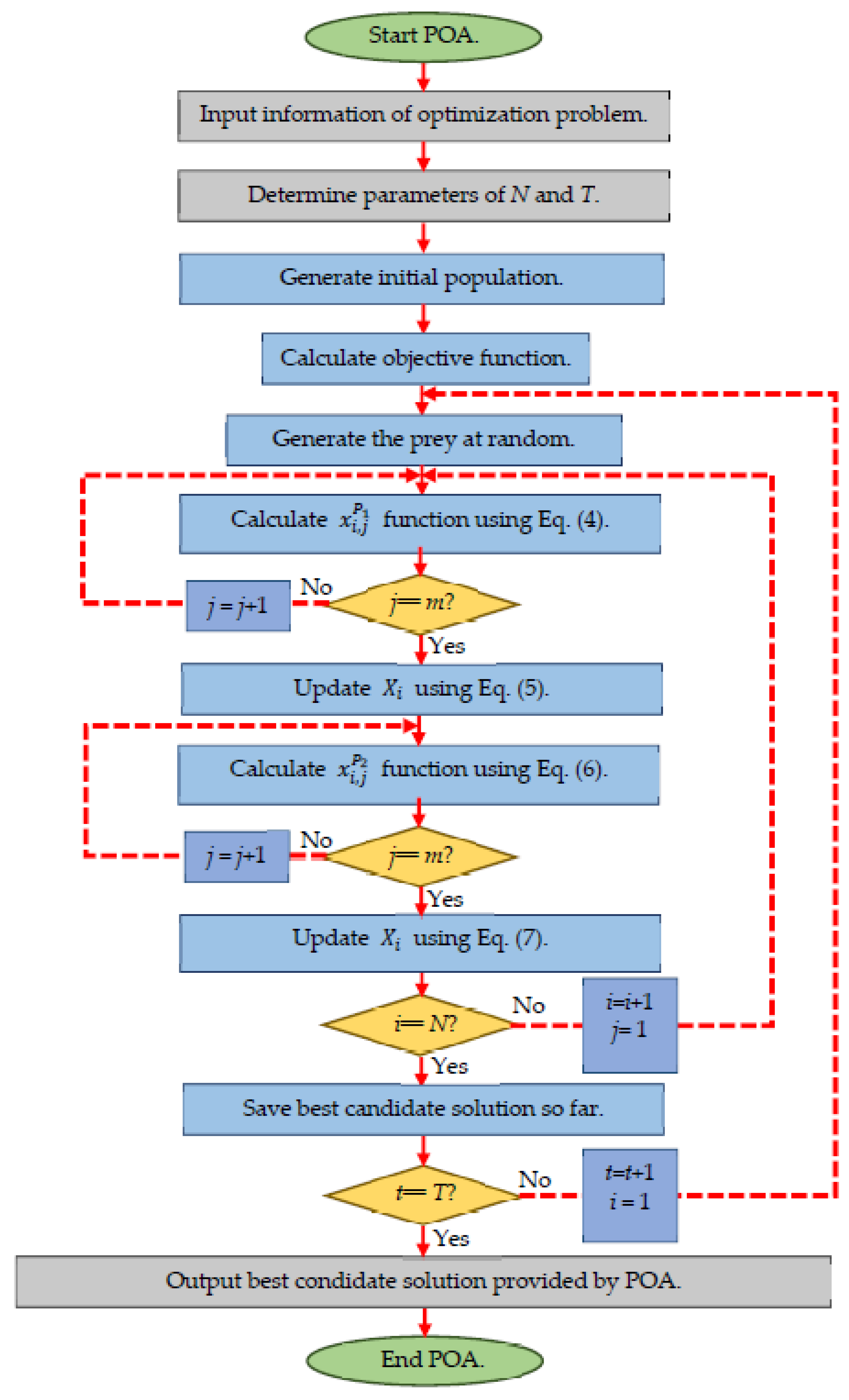
3.2.3. Steps Repetition, Pseudo-Code, and Flowchart of the Proposed POA

After all population members have been updated based on the first and second phases, based on the new status of the population and the values of the objective function, the best candidate solution so far will be updated. The algorithm enters the next iteration and the different steps of the proposed POA based on Equations (4)–(7) are repeated until the end of the complete execution. Finally, the best candidate solution obtained during the algorithm iterations is presented as a quasi-optimal solution to the given problem.
The various steps of the proposed POA are presented as a flowchart in Figure 1 and its pseudo-code in Algorithm 1.
Algorithm 1. Pseudo-code of POA.
Start POA.
1.Input the optimization problem information.
2.Determine the POA population size (N) and the number of iterations (T).
3.Initialization of the position of pelicans and calculate the objective function.
4.For t = 1:T
5.Generate the position of the prey at random.
6.For I = 1:N
7.Phase 1: Moving towards prey (exploration phase).
8.For j = 1:m
9.Calculate new status of the jth dimension using Equation (4).
10.End.
11.Update the ith population member using Equation (5).
12.Phase 2: Winging on the water surface (exploitation phase).
13.For j = 1:m.
14.Calculate new status of the jth dimension using Equation (6).
15.End.
16.Update the ith population member using Equation (7).
17.End.
18.Update best candidate solution.
19.End.
20.Output best candidate solution obtained by POA.
End POA.

3.3. Computational Complexity of the Proposed POA

In this subsection, the computational complexity of the proposed POA is calculated. The computational complexity of the proposed POA is based on four principles: algorithm initialization, evaluate the fitness function, generate prey, and solution updating. The computational complexity of the algorithm initialization processes is O ( N ) . In each iteration, each population member evaluates the objective function in each of the two phases. So, the computational complexity of the fitness function evaluation is O ( 2 · T · N ) . Given that prey is generated and evaluated at each iteration, O ( T ) + O ( T · m ) is the computational complexity of prey generation. In each iteration, the number of N population members that have m dimensions must be updated in two stages. Thus, the computational complexity of solutions updating is O ( 2 · T · N · m ) . Therefore, the total computational complexity of the proposed POA is equal to O ( N + T · ( 1 + m ) · ( 1 + 2 · N ) ) .

4. Simulation Studies and Results

In this section, the performance of the proposed POA in solving optimization problems is studied. For this purpose, POA is employed in solving twenty-three objective functions of different types of unimodal, high-dimensional multimodal, and fixed-dimensional multimodal. Details of the employed benchmark functions are specified in the Appendix A in Table A1, Table A2 and Table A3. In addition, the obtained optimization results from the proposed POA are compared with eight well-known optimization algorithms. These competing algorithms include (i) popular methods: Genetic Algorithm (GA) [19] and Particle Swarm Optimization (PSO) [13], (ii) popular and highly cited methods: Teaching–learning Based Optimization (TLBO) [14], Gray Wolf Optimization (GWO) [15], Whale Optimization Algorithm (WOA) [16], and Gravitational Search Algorithm (GSA) [22], and (iii) recently published methods: the Tunicate Swarm Algorithm (TSA) [17] and the Marine Predators Algorithm (MPA) [18]. Table 1 shows the values of the control parameters of these algorithms.
To evaluate the performance of the optimization algorithms, each of the competing algorithms, as well as the proposed POA in 20 independent implementations, each independent implementation containing 1000 iterations has been implemented on the objective functions. The simulation results are reported using four criteria: (i) the average of the best solutions obtained (avg), (ii) the standard deviation of the best solutions obtained (std), (iii) the best obtained candidate solution (bsf), and the median of the best solutions obtained (med). Two avg and std criteria are calculated using Equations (8) and (9).
a v g = 1 N r · i = 1 N r B C S i ,
s t d = 1 N r · i = 1 N r ( B C S i a v g ) 2 ,
where N r is the number of independent implementations and B C S i is the best candidate solution obtained in the ith independent implementation for a given problem.

4.1. Evaluation of Unimodal Functions

The objective functions of F1 to F7 are of the unimodal type. The proposed POA and eight competitor algorithms are implemented on these functions. Table 2 shows the results of optimizing the F1 to F7 functions. According to this table, the proposed algorithm in the F6 optimization converges to the global optimal of this function, i.e., zero. In addition, the proposed POA is the first best optimizer in solving F1, F2, F3, F4, F5, and F7 functions. The POA has produced results that are significantly more competitive and closer to the global optimal than the rival algorithms, according to the comparison of the performance of optimization algorithms.

4.2. Evaluation of High-Dimensional Multimodal Functions

To analyze the proposed POA and eight competitor algorithms in optimizing high-dimensional multi-modal functions, six objective functions, F8 to F13, have been selected. Table 3 shows the results of the implementation of POA and eight competitor algorithms on these objective functions. The proposed POA presents the global optimal with convergence to zero for F9 and F11. The proposed algorithm is the first best optimizer in providing quasi-optimal solutions for F8 and F10. TLBO is the best optimizer for F12 while POA is the sixth-best optimizer in solving this objective function. GSA is also the best optimizer in solving F13. Analysis of the simulation results shows that the proposed POA has an acceptable ability to solve this type of optimization problems and is competitive with eight compared algorithms.

4.3. Evaluation of Fixed-Dimensional Multimodal Functions

F14 through F23 are ten objective functions that assess optimization algorithms’ capacity to tackle fixed-dimensional multimodal issues. The results of optimizing these objective functions using the proposed POA and eight competitor techniques are shown in Table 4. The proposed POA in optimizing F14 and F17 has been capable of converging to the global optimal of these functions. POA is the first best optimizer in solving F15, F19, F20 F21, F22, and F23. In optimizing the functions of F16, and F18 although the performance of the POA is similar to some competitor algorithms in the avg criterion, it has a better std criterion. Therefore, the proposed POA is more efficient to solve these objective functions. Analysis of the simulation results shows that the proposed POA has a higher ability to solve F14 to F23 fixed-dimensional multimodal optimization problems than the eight competitor algorithms.
The performance of the optimization algorithms and the proposed POA in solving the objective functions F1 to F23 are presented in Figure 2 as a boxplot.

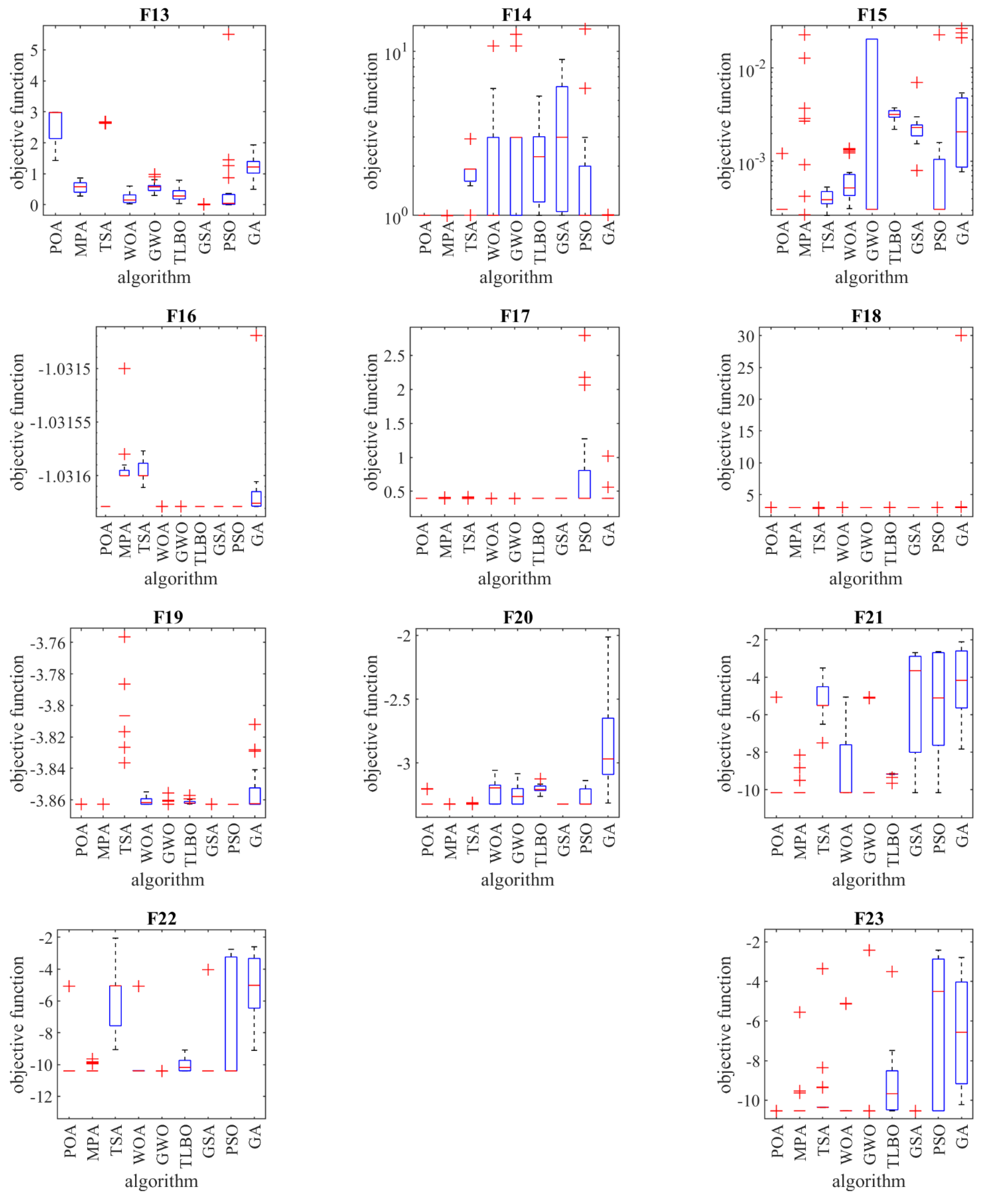
4.4. Statistical Analysis

The use of average and std indices to report the optimization results of objective functions gives useful information about the comparison and performance of optimization techniques. Nevertheless, even after numerous separate executions, it is always conceivable that the superiority of one algorithm over several other algorithms be random. Therefore, in this subsection, a statistical analysis called a Wilcoxon sum rank test [29] is presented to show the superiority of the POA over eight competitor algorithms from a statistical point of view. The Wilcoxon sum rank test is a non-parametric statistical test that compares the similarity of two dependent samples. This test determines whether the difference between the two samples is statistically significant or not.
In the Wilcoxon sum rank test, an index called a p-value has been employed to determine the statistically significant difference between the performance of the two algorithms in optimizing different groups of objective functions. The simulation results of this test for the proposed POA with eight competitor algorithms are presented in Table 5. In this table, in cases where a p -value is less than 0.05, the proposed POA has a significant superiority over the competitor algorithm in that group of objective functions.

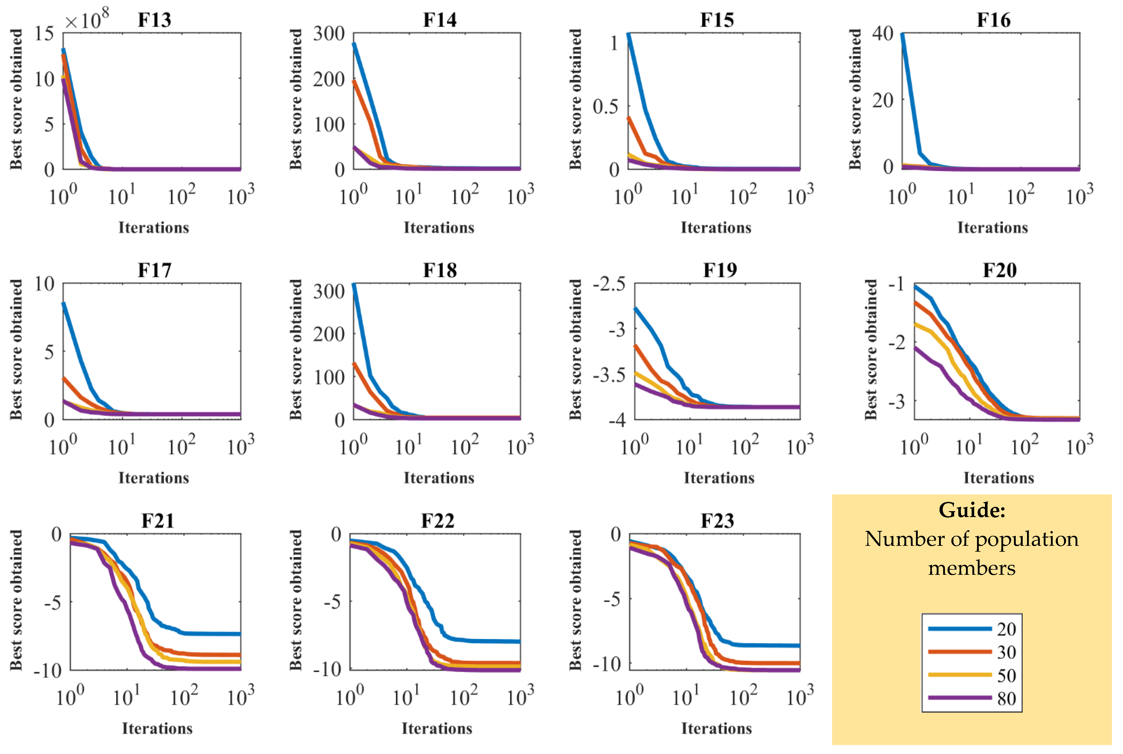
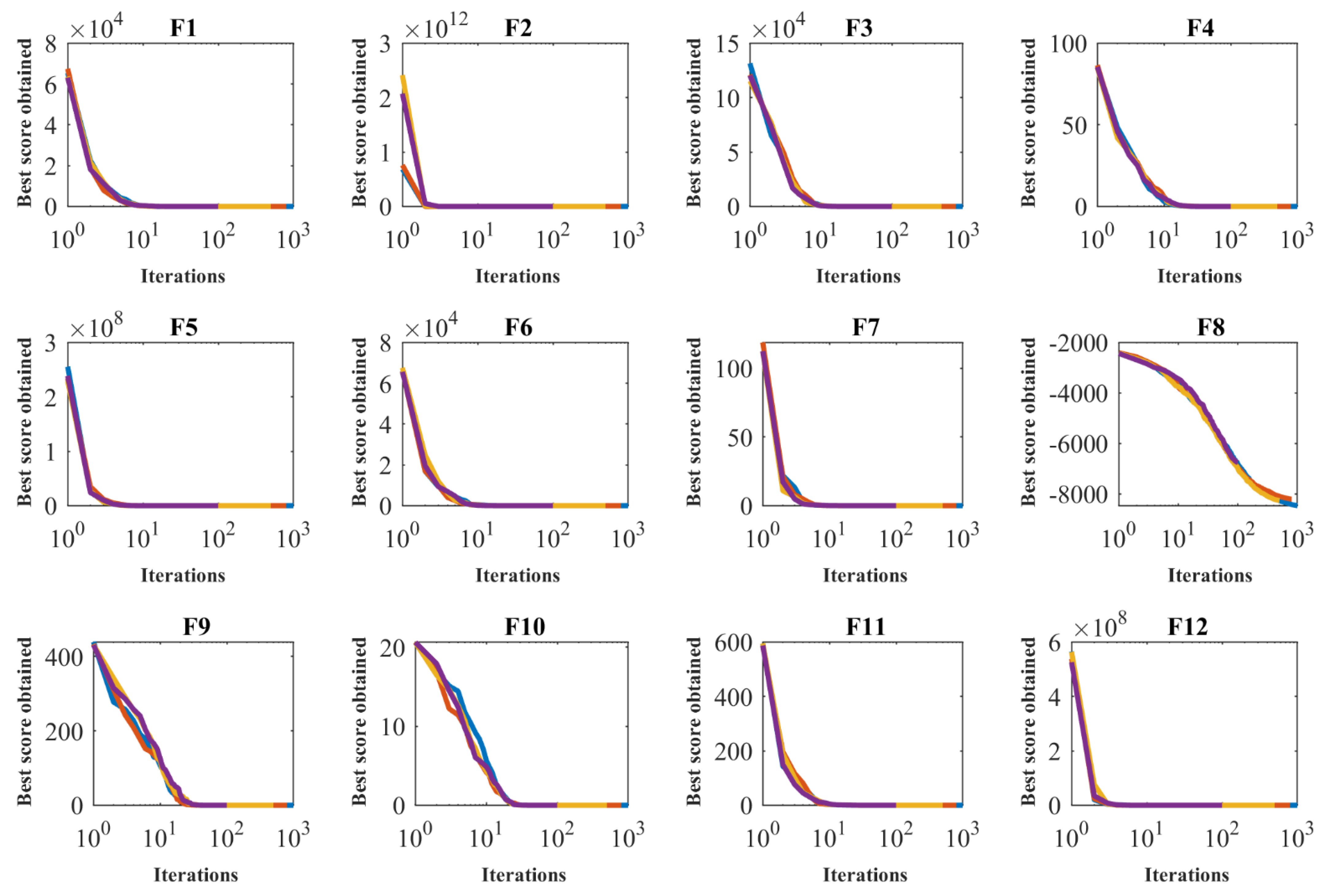
4.5. Sensitivity Analysis

The proposed POA is a population-based algorithm that converges to a quasi-optimal solution in an iterative process for a given optimization problem. Therefore, the values of these two parameters affect the performance of POA. In addition, the value of the parameter R in Equation (6) can also significantly affect the performance of the POA.
In this subsection, it has been studied the sensitivity analysis of the proposed POA with respect to the three parameters, namely the population number N , the maximum number of iterations T , and parameter R . There is not a general rule for setting values of N and T , but their values choice depends on factors such as the nature of the problem, the number of variables, constraints, and so on. Experimental knowledge and familiarity with the given optimization problem are very influential in choosing these two parameters. However, if there is no necessary knowledge and familiarity with the given problem, the values of these two parameters can be adjusted based on trial and error.
To evaluate the performance sensitivity of the proposed algorithm to the parameter N , POA for different populations of 20, 30, 50, and 80 members was implemented on the F1 to F23 objective functions. Table 6 shows the simulation results of the sensitivity analysis of the proposed POA to the parameter N . What can be deduced from this table is that the increase in population members has led to an increase in the exploratory power of the algorithm in search of search space and the discovery of more optimal areas. Therefore, as the number of population members increases, the value of the objective function decreases. Figure 3 shows the behavior of the convergence curves of the proposed POA in the sensitivity analysis to the parameter N .
To analyze the sensitivity of the proposed algorithm to the parameter T , POA is applied to solve the objective functions F1 to F23 for the maximum number of iterations of 100, 500, 800, and 1000. The simulation results of the sensitivity of the proposed POA to the parameter T are presented in Table 7. Based on the results of this table, it was found that increasing the number of iterations of the algorithm gives more time to the population members to converge towards the optimal solution. Increasing the algorithm’s maximum number of iterations improves the algorithm’s exploitation power, allowing it to produce better solutions. The simulation results reveal that increasing the algorithm’s maximum number of iterations reduces the values of the goal functions. Figure 4 depicts the behavior of convergence curves under the effect of sensitivity analysis of the proposed POA to the T.
In order to analyze the sensitivity of POA to the parameter R , it should be noted that the coefficient “ R · ( 1 t / T ) ” indicates that in each iteration, the maximum change for each member of the population is “ R · ( 1 t / T ) ” times its current position. Therefore, the value of the parameter R in this coefficient must be less than one. The proposed POA for different values of R equal to 0.1, 0.2, 0.3, 0.4, 0.5, 0.6, 0.7, 0.8, 0.9, and 1 is employed in the optimization of the F1 to F23 function. The optimization results of F1 to F23 functions for different values of parameter R are reported in Table 8. The results of this sensitivity analysis show that the POA has a very low sensitivity to changes in the parameter R and in most cases provides the same solution. In optimizing of the functions F6, F9, F10, F11, F14, F15, F16, F17, F18, and F19, the different selected values for the parameter R had no effect on POA performance. In the general analysis and comparison of the results, it was found that POA has the best performance for the value of R equal to 0.2.

5. Discussion

Exploration power and exploitation power are two key and influential indicators of optimization algorithms’ success in obtaining solutions to optimization issues.
Exploitation power demonstrates the ability of the algorithm to search locally and converge as much as possible towards the global optimal. According to this concept, a good optimization algorithm should be able to accurately scan the space around the identified optimal area to provide a suitable quasi-optimal solution. Therefore it can be said that, compared to the performance of several optimization algorithms, the algorithm that converges to a better solution has a higher exploitation power. The F1 to F7 objective functions, which are of the unimodal type, have only one main peak and are therefore suitable for evaluating the exploitation power. The simulation results of these objective functions reported in Table 2 indicate the high exploitation ability of the proposed POA in local search and suitable convergence towards the global optimal. Analysis of the optimization results of these objective functions indicates very competitive and significant superiority of the proposed POA in the exploitation power and in providing a quasi-optimal solution over eight competing algorithms.
Exploration power demonstrates the ability of an algorithm to global search in problem-solving space and cross local optimal areas to discover the main optimal area. Accordingly, in comparing several optimization algorithms, an algorithm that scans the search space more accurately and is able to identify the area containing the global optimal has a higher exploration power. Exploration power is especially important in optimizing problems that have several local optimal in addition to the global optimal. F8 to 23 multimodal objective functions have this feature and are therefore suitable for evaluating the exploration power of optimization algorithms. The optimization results of these objective functions presented in Table 3 and Table 4 show that the proposed POA has a high exploration power for the global search in the problem-solving space and has been able to identify the optimal local area. Comparison and analysis of simulation results of F8 to F23 functions indicate the high exploration ability of POA compared to eight competing algorithms.

6. POA for Real-World Applications

In order to assess the effectiveness of POA in real-world purposes, this optimizer has been utilized to solve four engineering problems: pressure vessel design, speed reducer design, welded beam design, and tension/compression spring design.

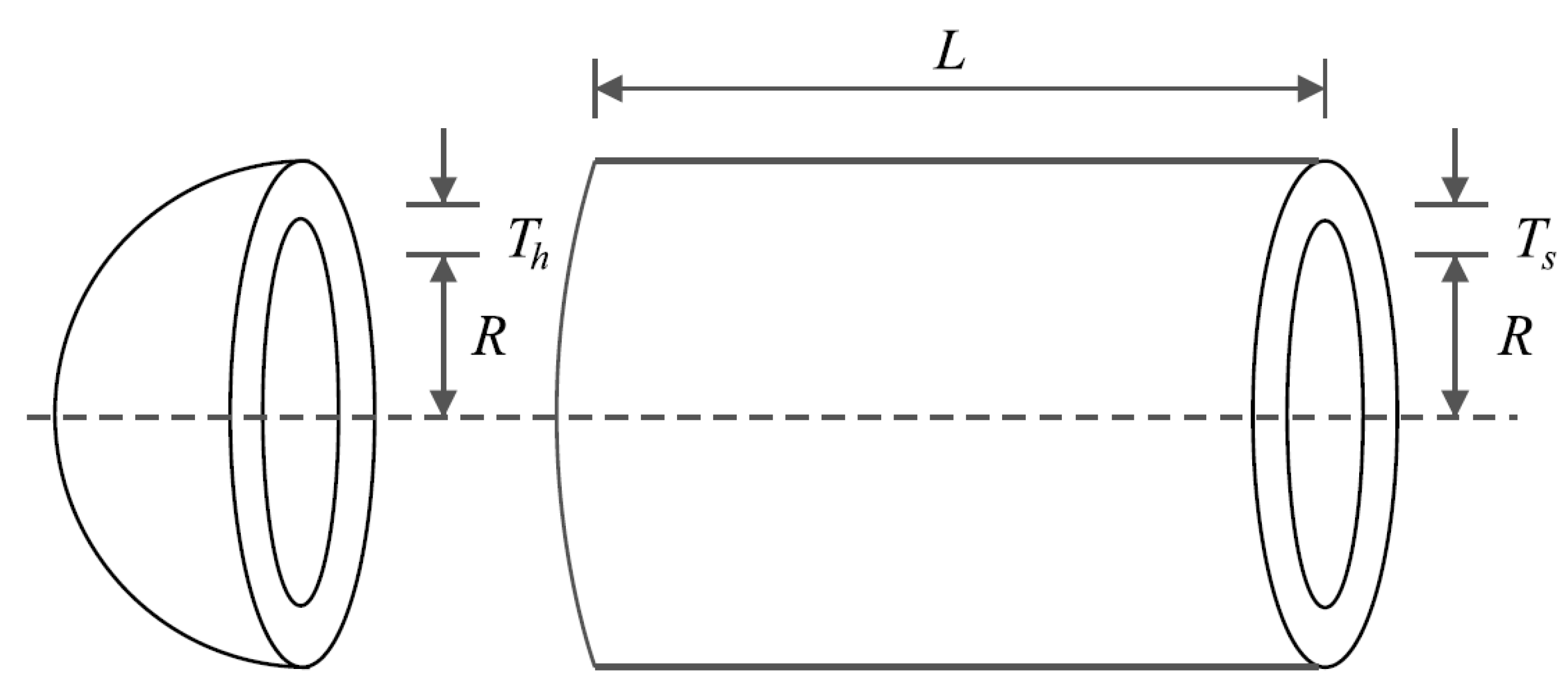
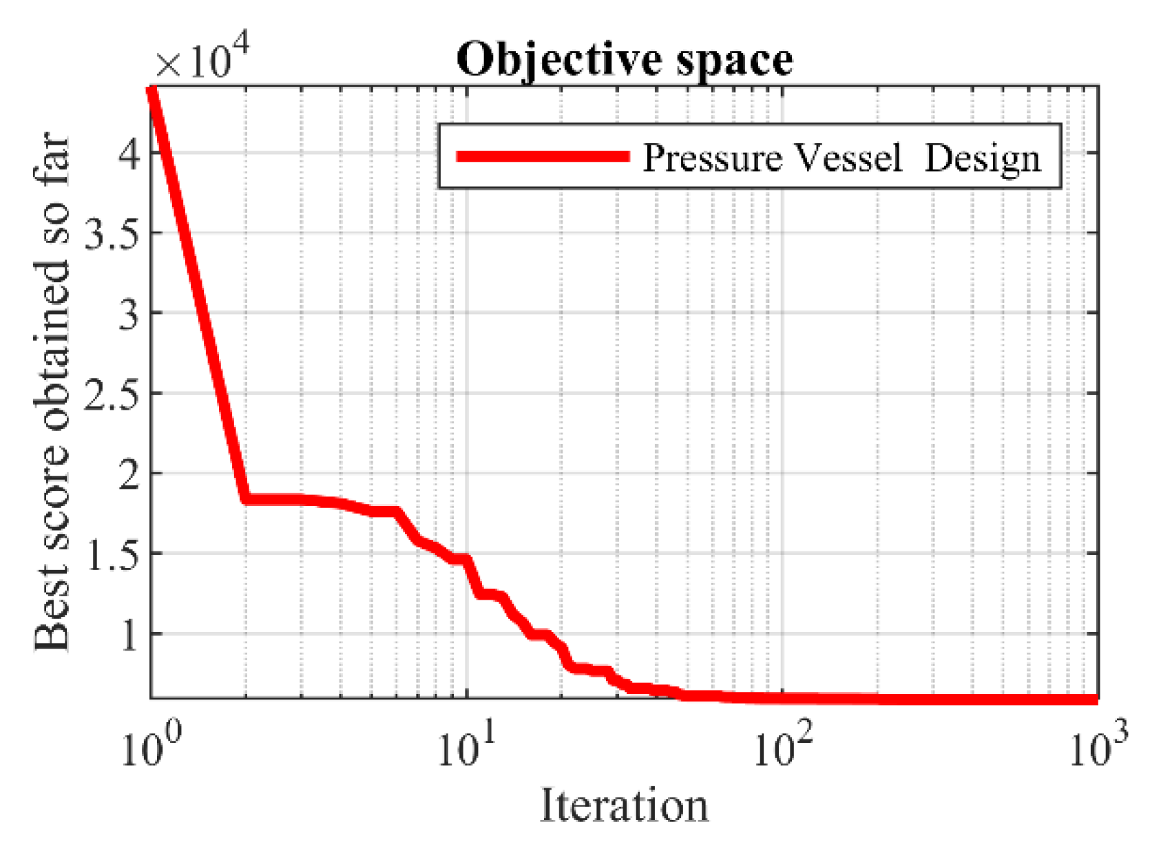
6.1. Pressure Vessel Design

Pressure vessel design [30] is a minimization problem whose schematic is shown in Figure 5. The mathematical model of this problem is as follows:
Consider  X = [ x 1 ,   x 2 ,   x 3 ,   x 4 ] = [ T s ,   T h ,   R ,   L ] .
Minimize  f   ( x ) = 0.6224 x 1 x 3 x 4 + 1.778 x 2 x 3 2 + 3.1661 x 1 2 x 4 + 19.84 x 1 2 x 3 .
Subject to:
g 1   ( x ) = x 1 + 0.0193 x 3     0 ,
g 2   ( x ) = x 2 + 0.00954 x 3   0 ,  
g 3   ( x ) = π x 3 2 x 4 4 3 π x 3 3 + 1296000   0 ,  
g 4   ( x ) = x 4 240     0 .  
With
0 x 1 , x 2 100 ,   a n d   10 x 3 , x 4 200 .
Figure 5. Schematic of pressure vessel design.
Sensors 22 00855 g005
The optimization results of this problem are presented in Table 9. POA provides the optimal solution with the values of the variables equal to (0.778035, 0.384607, 40.31261, and 199.9972) and the value of the objective function (5883.0278). The statistical results of the performance of competing and POA algorithms are reported in Table 10. Based on these results, POA, with better statistical indicators, has outperformed competing algorithms. Figure 6 shows the POA convergence curve in the pressure vessel design solution.

6.2. Speed Reducer Design Problem

Speed reducer design [31,32] is a weight minimization problem for a speed reducer. The schematic of this problem is shown in Figure 7 and the mathematical model of this problem is as follows:
Consider X = [ x 1 ,   x 2 ,   x 3 ,   x 4 ,   x 5 , x 6 , x 7 ] = [ b ,   m ,   p ,   l 1 ,   l 2 ,   d 1 ,   d 2 ] .
Minimize f   ( x ) = 0.7854 x 1 x 2 2 ( 3.3333 x 3 2 + 14.9334 x 3 43.0934 ) 1.508 x 1 ( x 6 2 + x 7 2 ) + 7.4777 ( x 6 3 + x 7 3 ) + 0.7854 ( x 4 x 6 2 + x 5 x 7 2 ) .
Subject to:
g 1   ( x ) = 27 x 1 x 2 2 x 3 1     0 ,  
g 2   ( x ) = 397.5 x 1 x 2 2 x 3 1   0 ,  
g 3   ( x ) = 1.93 x 4 3 x 2 x 3 x 6 4 1   0 ,  
g 4   ( x ) = 1.93 x 5 3 x 2 x 3 x 7 4 1     0 ,  
g 5 ( x ) = 1 110 x 6 3 ( 745 x 4 x 2 x 3 ) 2 + 16.9 × 10 6 1   0 ,  
g 6 ( x ) = 1 85 x 7 3 ( 745 x 5 x 2 x 3 ) 2 + 157.5 × 10 6 1     0 ,  
g 7   ( x ) = x 2 x 3 40 1     0 ,  
g 8   ( x ) = 5 x 2 x 1 1     0 ,  
g 9   ( x ) = x 1 12 x 2 1     0 ,  
g 10   ( x ) = 1.5 x 6 + 1.9 x 4 1     0 ,  
g 11   ( x ) = 1.1 x 7 + 1.9 x 5 1     0 .
With
2.6 x 1 3.6 ,   0.7 x 2 0.8 ,   17 x 3 28 ,   7.3 x 4 8.3 ,   7.8 x 5 8.3 ,   2.9 x 6 3.9 ,   a n d   5 x 7 5.5 .
Figure 7. Schematic of speed reducer design.
Sensors 22 00855 g007
The values obtained from different algorithms are reported in Table 11. Based on these results, it is clear that POA has provided the optimal solution to this problem with the values of the variables equal to (3.5, 0.7, 17, 7.3, 7.88, 3.350215, and 5.286683) and the value of the objective function (2996.3482). The statistical results obtained from the implementation of competitor algorithms and POA on the speed reducer design problem are presented in Table 12. The analysis of these results indicates the superiority of POA in the effective solution of this problem due to having better values for statistical indicators. The POA convergence curve during speed reducer design optimization is shown in Figure 8.

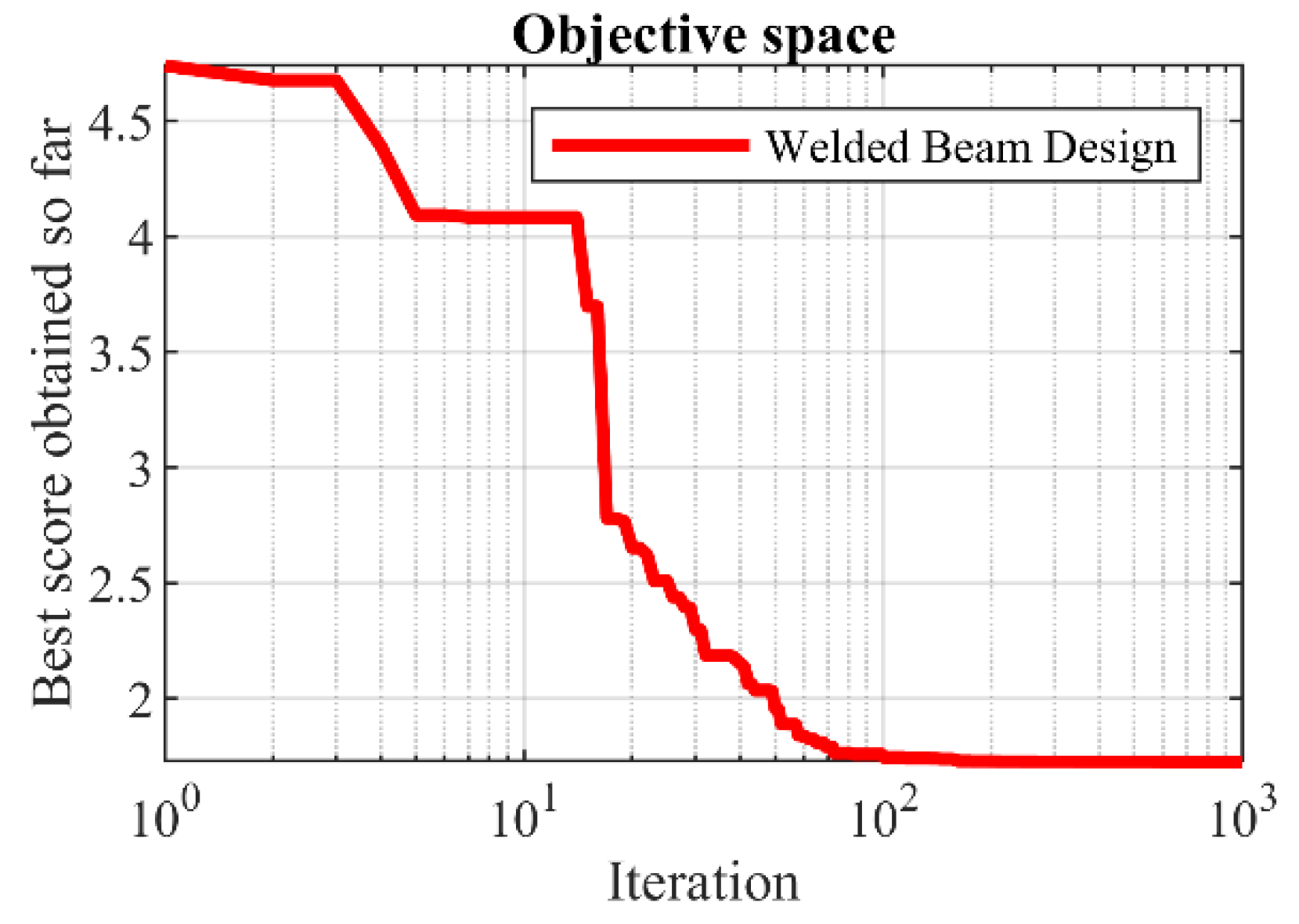
6.3. Welded Beam Design

Welded beam design [16] is a minimizing problem of the fabrication cost of welded beam which the schematic of this problem is shown in Figure 9. The mathematical model of this problem is as follows:
Consider X = [ x 1 ,   x 2 ,   x 3 ,   x 4 ] = [ h ,   l ,   t ,   b ] .
Minimize f   ( x ) = 1.10471 x 1 2 x 2 + 0.04811 x 3 x 4   ( 14.0 + x 2 ) .
Subject to:
g 1   ( x ) = τ ( x ) 13600     0 ,  
g 2   ( x ) = σ ( x ) 30000     0 ,  
g 3   ( x ) = x 1 x 4   0 ,  
g 4   ( x ) = 0.10471 x 1 2 + 0.04811 x 3 x 4   ( 14 + x 2 ) 5.0     0 ,  
g 5 ( x ) = 0.125 x 1   0 ,  
g 6 ( x ) = δ   ( x ) 0.25     0 ,  
g 7   ( x ) = 6000 p c   ( x )     0 .  
Where
τ ( x ) = τ + ( 2 τ τ ) x 2 2 R + ( τ ) 2 ,  
τ = 6000 2 x 1 x 2 ,  
τ = M R J ,  
M = 6000 ( 14 + x 2 2 ) ,  
R = x 2 2 4 + ( x 1 + x 3 2 ) 2 ,  
J = 2 { x 1 x 2 2 [ x 2 2 12 + ( x 1 + x 3 2 ) 2 ] } ,  
σ ( x ) = 504000 x 4 x 3 2  
δ   ( x ) = 65856000 ( 30 · 10 6 ) x 4 x 3 3 ,  
p c   ( x ) = 4.013 ( 30 · 10 6 ) x 3 2 x 4 6 36 196 ( 1 x 3 28 30 · 10 6 4 ( 12 · 10 6 ) ) .  
With
0.1 x 1 ,   x 4 2   a n d   0.1 x 2 ,   x 3 10 .
Figure 9. Schematic of welded beam design.
Sensors 22 00855 g009
The optimization results of the welded beam design problem are presented in Table 13. The POA provides the optimal solution to this problem by assigning the values of the variables equal to (0.205719, 3.470104, 9.038353, and 0.205722) and the value of the objective function (1.725021). The statistical results of performance of POA and eight competitor algorithms in optimizing this problem are reported in Table 14. Comparison of the results shows that POA has the superior ability to introduce optimal values of variables over eight competitor algorithms. The POA convergence curve to the optimal solution of the welded beam design problem is shown in Figure 10.

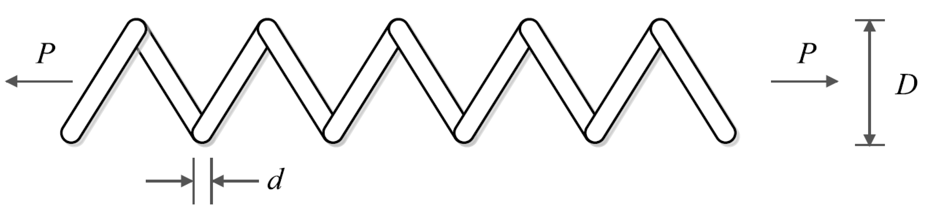
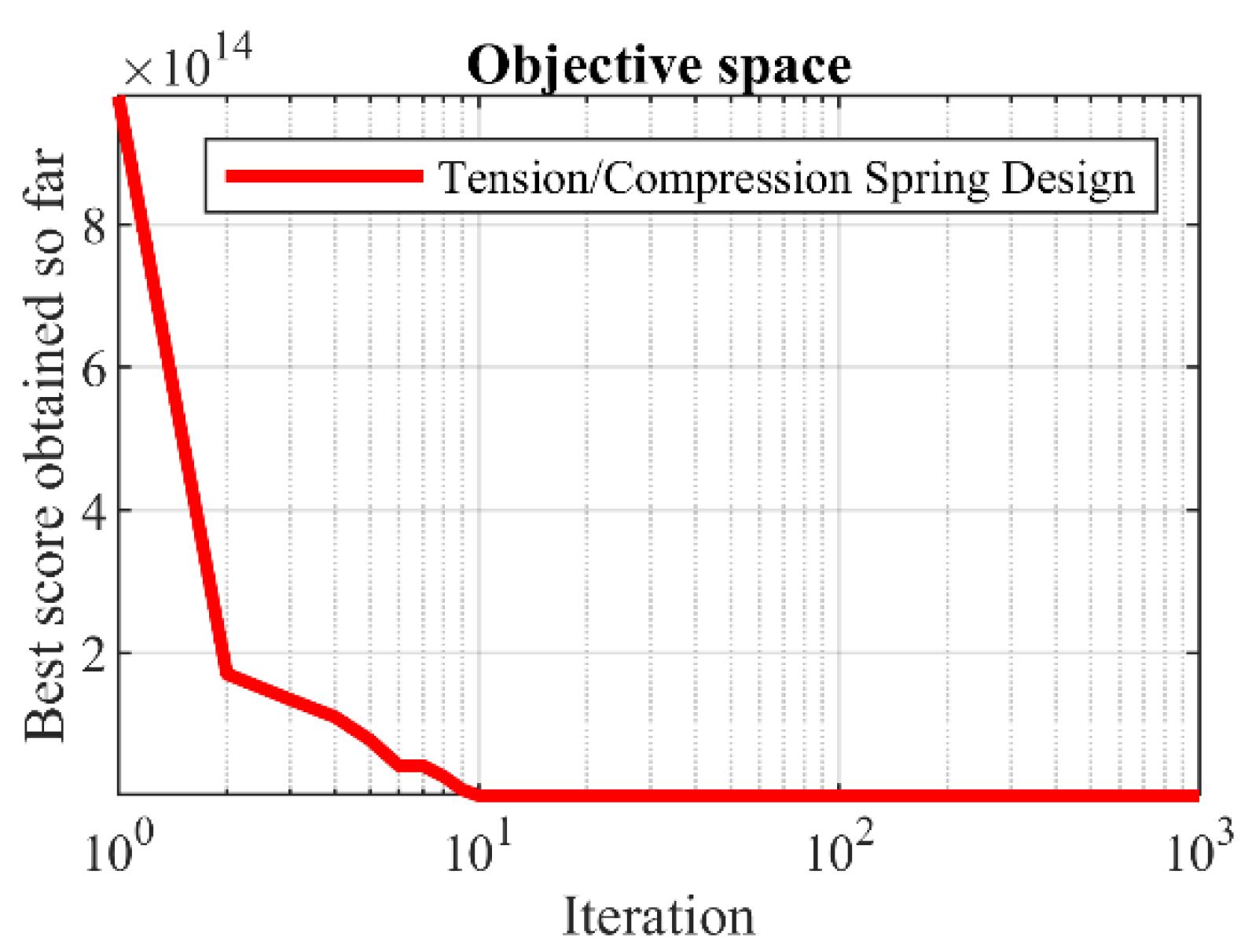
6.4. Tension/Compression Spring Design Problem

Tension/compression spring design [16] is a weight minimization problem, a schematic of which is shown in Figure 11. The mathematical model of this problem is as follows:
Consider X = [ x 1 ,   x 2 ,   x 3   ] = [ d ,   D ,   P ] .
Minimize f   ( x ) = ( x 3 + 2 ) x 2 x 1 2 .
Subject to:
g 1   ( x ) = 1 x 2 3 x 3 71785 x 1 4     0 ,  
g 2   ( x ) = 4 x 2 2 x 1 x 2 12566 ( x 2 x 1 3 ) + 1 5108 x 1 2 1   0 ,  
g 3   ( x ) = 1 140.45 x 1 x 2 2 x 3   0 ,
g 4   ( x ) = x 1 + x 2 1.5 1     0 .
With
0.05 x 1 2 ,   0.25 x 2 1.3   a n d   2   x 3 15 .
Figure 11. Schematic of tension/compression spring design.
Sensors 22 00855 g011
The implementation results of POA and eight competitor algorithms on solving tension/compression spring design are reported in Table 15. Based on the results, it is clear that POA has provided the optimal solution by presenting the values of the variables equal to (0.051892, 0.361608, and 11.00793) and the value of the objective function (0.012666). The statistical results of the performance of the employed algorithms are presented in Table 16. What can be deduced from this table is that POA is a more effective optimizer for solving the tension/compression spring design problem against eight competitor algorithms by providing better statistical indicators. The convergence curve of POA during convergence to the optimal solution of this problem is shown in Figure 12.

6.5. The POA’s Applicability in Image Processing and Sensor Networks

Interconnected sensors collect huge amounts of data which are frequently useful in a variety of contexts. In today’s digital transformation era, numerous sorts of sensors and networks reinforce the usage of artificial intelligence and big data science. These data are primarily unstructured and well specified within the context of artificial intelligence, machine learning, data science, and big data. Data from medical images, traceability of infected patients, environmental monitoring, mobility in public transport, etc., usually georeferenced, are very interesting for the above research. These huge amounts of data come from a variety of sources, ranging from social media to IoT sensors. For these sorts of observations, classical methods for structured data analysis are insufficient and inadequate for discovering relevant knowledge and obtaining information. As a result, artificial intelligence approaches, such as the use of the proposed POA for various applications in sensor and image processing networks, are becoming increasingly important. In general, the application of the proposed POA in solving optimization problems might enable a broad range of future tasks in image processing, wireless sensor networks, signal denoising, machine learning, power systems, artificial intelligence, big data, COVID-19 modeling, data mining, feature selection, and other benchmark functions.

7. Conclusions and Future Works

In this paper, a new swarm-based optimization algorithm called the Pelican Optimization Algorithm (POA) was presented. The fundamental inspiration of the proposed POA is the strategy and behavior of pelicans during hunting. These behaviors include diving towards their prey and fluttering wings on the surface of the water. The various steps of POA were described and then its mathematical modeling was presented for use in solving optimization problems. The proposed algorithm was tested by solving twenty-three objective functions belonging to unimodal, high-dimensional multimodal, and fixed-dimensional multimodal. Additionally, to further analyze the capabilities of the proposed algorithm, the optimization results obtained from POA are compared with the performance of eight well-known algorithms, including WOA, TSA, GWO, MPA, GSA, GA, TLBO, and PSO. The optimization results of unimodal functions indicated the high exploitation power of the proposed POA in converging towards the global optimal solution. The simulation results of these functions showed that POA has significant superiority over eight competitor algorithms in solving unimodal problems. The simulation outcomes of multimodal functions demonstrated the suggested POA’s high exploration power in effective checking of the search space and finding of the optimal area. The simulation results demonstrated that the POA approach outperformed eight competitor algorithms in handling multimodal optimization issues. Based on the simulation results, it is possible to infer that the suggested POA is highly efficient in addressing optimization issues and is far more competitive and superior to similar methods. In addition, POA was employed for solving four engineering design problems, including pressure vessel design, speed reducer design, welded beam design, and tension/compression spring design. The simulation results showed that POA has a satisfactory performance in effectively solving design problems in real-world applications.
The authors provide several research directions for future studies with respect to this paper. Among the specific research potentials of the proposed method are the development of binary and multi-objective versions of POA. Furthermore, the authors’ ideas for future research include the application of the POA in tackling optimization issues in various science fields and real-world challenges. Note that the proposed POA might enable a broad range of future tasks. This includes applying this algorithm in numerous applications such as, e.g., image processing, wireless sensor networks, signal denoising, machine learning, power systems, artificial intelligence, big data, COVID-19 modeling, data mining, feature selection, and other benchmark functions. Like all stochastic optimization techniques, one of the limitations of the proposed POA is that new optimizers may be developed in the future that will perform better than POA in some real applications. Additionally, due to the stochastic nature of the POA solution method, it cannot be guaranteed that the solutions obtained using POA for optimization problems are exactly equal to the global optimum for all optimization problems.

Author Contributions

Conceptualization, M.D. and P.T.; methodology, P.T.; software, M.D.; validation, P.T. and M.D.; formal analysis, M.D.; investigation, P.T.; resources, P.T.; data curation, M.D.; writing—original draft preparation, P.T. and M.D.; writing—review and editing, M.D.; visualization, P.T.; supervision, P.T.; project administration, M.D.; funding acquisition, P.T. All authors have read and agreed to the published version of the manuscript.

Funding

This research was funded by the Project of Excellence of Faculty of Science, University of Hradec Králové, grant number 2210/2022-2023.

Institutional Review Board Statement

Not applicable.

Informed Consent Statement

Not applicable.

Data Availability Statement

Not applicable.

Acknowledgments

The authors thank University of Hradec Králové for support.

Conflicts of Interest

The authors declare no conflict of interest.

Appendix A

The information of the objective functions used in the simulation section is presented in Table A1, Table A2 and Table A3.
Table A1. Unimodal functions.
Objective FunctionRangeDimensions F m i n
F 1 ( x ) = i = 1 m x i 2 [ 100 ,   100 ] 300
F 2 ( x ) = i = 1 m | x i | + i = 1 m | x i | [ 10 ,   10 ] 300
F 3 ( x ) = i = 1 m ( j = 1 i x i ) 2 [ 100 ,   100 ] 300
F 4 ( x ) = m a x { | x i | ,     1 i m   } [ 100 ,   100 ] 300
F 5 ( x ) = i = 1 m 1 [ 100 ( x i + 1 x i 2 ) 2 + ( x i 1 ) 2 ) ] [ 30 ,   30 ] 300
F 6 ( x ) = i = 1 m ( [ x i + 0.5 ] ) 2 [ 100 ,   100 ] 300
F 7 ( x ) = i = 1 m i x i 4 + r a n d o m ( 0 , 1 ) [ 1.28 ,   1.28 ] 300
Table A2. High-dimensional multimodal functions.
Objective FunctionRangeDimensionsFmin
F 8 ( x ) = i = 1 m x i   sin ( | x i | ) [ 500 ,   500 ] 30−12,569
F 9 ( x ) = i = 1 m [   x i 2 10 cos ( 2 π x i ) + 10 ] [ 5.12 ,   5.12 ] 300
F 10 ( x ) = 20 exp ( 0.2 1 m i = 1 m x i 2 ) exp ( 1 m i = 1 m cos ( 2 π x i ) ) + 20 + e [ 32 ,   32 ] 300
F 11 ( x ) = 1 4000 i = 1 m x i 2 i = 1 m cos ( x i i ) + 1 [ 600 ,   600 ] 300
F 12 ( x ) = π m   { 10 sin ( π y 1 ) + i = 1 m ( y i 1 ) 2 [ 1 + 10 sin 2 ( π y i + 1 ) ] + ( y n 1 ) 2 } + i = 1 m u ( x i , 10 , 100 , 4 ) , where
u ( x i , a , i , n ) = { k ( x i a ) n ,                               x i > a ; 0 ,                                       a   x i   a k ( x i a ) n ,                       x i < a . ;
[ 50 ,   50 ] 300
F 13 ( x ) = 0.1 {   sin 2 ( 3 π x 1 ) + i = 1 m ( x i 1 ) 2 [ 1 + sin 2 ( 3 π x i + 1 ) ] + ( x n 1 ) 2 [ 1 + sin 2 ( 2 π x m ) ] } + i = 1 m u ( x i , 5 , 100 , 4 ) , [ 50 ,   50 ] 300
Table A3. Fixed-dimensional multimodal functions.
Objective FunctionRangeDimensionsFmin
F 14 ( x ) = ( 1 500 + j = 1 25 1 j + i = 1 2 ( x i a i j ) 6 ) 1 [ 65.53 ,   65.53 ] 20.998
F 15 ( x ) = i = 1 11 [ a i x 1 ( b i 2 + b i x 2 ) b i 2 + b i x 3 + x 4 ] 2 [ 5 ,   5 ] 40.00030
F 16 ( x ) = 4 x 1 2 2.1 x 1 4 + 1 3 x 1 6 + x 1 x 2 4 x 2 2 + 4 x 2 4 [ 5 ,   5 ] 2−1.0316
F 17 ( x ) = ( x 2 5.1 4 π 2 x 1 2 + 5 π x 1 6 ) 2 + 10 ( 1 1 8 π ) cos x 1 + 10 [-5, 10] × [0, 15]20.398
F 18 ( x ) = [ 1 + ( x 1 + x 2 + 1 ) 2 ( 19 14 x 1 + 3 x 1 2 14 x 2 + 6 x 1 x 2 + 3 x 2 2 ) ] · [ 30 + ( 2 x 1 3 x 2 ) 2 · ( 18 32 x 1 + 12 x 1 2 + 48 x 2 36 x 1 x 2 + 27 x 2 2 ) ] [ 5 ,   5 ] 23
F 19 ( x ) = i = 1 4 c i   exp ( j = 1 3 a i j ( x j P i j ) 2 ) [ 0 ,   1 ] 3−3.86
F 20 ( x ) = i = 1 4 c i   exp ( j = 1 6 a i j ( x j P i j ) 2 ) [ 0 ,   1 ] 6−3.22
F 21 ( x ) = i = 1 5 [ ( X a i ) ( X a i ) T + 6 c i ] 1 [ 0 ,   10 ] 4−10.1532
F 22 ( x ) = i = 1 7 [ ( X a i ) ( X a i ) T + 6 c i ] 1 [ 0 ,   10 ] 4−10.4029
F 23 ( x ) = i = 1 10 [ ( X a i ) ( X a i ) T + 6 c i ] 1 [ 0 ,   10 ] 4−10.5364

References

  1. Farshi, T.R. Battle royale optimization algorithm. Neural Comput. Appl. 2021, 33, 1139–1157. [Google Scholar] [CrossRef]
  2. Ray, T.; Liew, K.-M. Society and civilization: An optimization algorithm based on the simulation of social behavior. IEEE Trans. Evol. Comput. 2003, 7, 386–396. [Google Scholar] [CrossRef]
  3. Francisco, M.; Revollar, S.; Vega, P.; Lamanna, R. A comparative study of deterministic and stochastic optimization methods for integrated design of processes. IFAC Proc. Vol. 2005, 38, 335–340. [Google Scholar] [CrossRef] [Green Version]
  4. Hashim, F.A.; Hussain, K.; Houssein, E.H.; Mabrouk, M.S.; Al-Atabany, W. Archimedes optimization algorithm: A new metaheuristic algorithm for solving optimization problems. Appl. Intell. 2021, 51, 1531–1551. [Google Scholar] [CrossRef]
  5. Abualigah, L.; Yousri, D.; Abd Elaziz, M.; Ewees, A.A.; Al-qaness, M.A.; Gandomi, A.H. Aquila Optimizer: A novel meta-heuristic optimization Algorithm. Comput. Ind. Eng. 2021, 157, 107250. [Google Scholar] [CrossRef]
  6. Iba, K. Reactive power optimization by genetic algorithm. IEEE Trans. Power Syst. 1994, 9, 685–692. [Google Scholar] [CrossRef]
  7. Geetha, K.; Anitha, V.; Elhoseny, M.; Kathiresan, S.; Shamsolmoali, P.; Selim, M.M. An evolutionary lion optimization algorithm-based image compression technique for biomedical applications. Expert Syst. 2021, 38, e12508. [Google Scholar] [CrossRef]
  8. Yadav, R.K.; Mahapatra, R.P. Hybrid metaheuristic algorithm for optimal cluster head selection in wireless sensor network. Pervasive Mob. Comput. 2021, 79, 101504. [Google Scholar] [CrossRef]
  9. Cano Ortega, A.; Sánchez Sutil, F.J.; De la Casa Hernández, J. Power factor compensation using teaching learning based optimization and monitoring system by cloud data logger. Sensors 2019, 19, 2172. [Google Scholar] [CrossRef] [Green Version]
  10. Todorčević, V. Harmonic Quasiconformal Mappings and Hyperbolic Type Metrics; Springer: Berlin/Heidelberg, Germany, 2019. [Google Scholar]
  11. Debnath, P.; Konwar, N.; Radenovic, S. Metric Fixed Point Theory: Applications in Science, Engineering and Behavioural Sciences; Springer: Berlin/Heidelberg, Germany, 2021. [Google Scholar]
  12. Wolpert, D.H.; Macready, W.G. No free lunch theorems for optimization. IEEE Trans. Evol. Comput. 1997, 1, 67–82. [Google Scholar] [CrossRef] [Green Version]
  13. Kennedy, J.; Eberhart, R. Particle swarm optimization. In Proceedings of the ICNN’95—International Conference on Neural Networks, Perth, Australia, 27 November–1 December 1995; Volume 4, pp. 1942–1948. [Google Scholar]
  14. Rao, R.V.; Savsani, V.J.; Vakharia, D. Teaching–learning-based optimization: A novel method for constrained mechanical design optimization problems. Comput. Aided Des. 2011, 43, 303–315. [Google Scholar] [CrossRef]
  15. Mirjalili, S.; Mirjalili, S.M.; Lewis, A. Grey wolf optimizer. Adv. Eng. Softw. 2014, 69, 46–61. [Google Scholar] [CrossRef] [Green Version]
  16. Mirjalili, S.; Lewis, A. The whale optimization algorithm. Adv. Eng. Softw. 2016, 95, 51–67. [Google Scholar] [CrossRef]
  17. Kaur, S.; Awasthi, L.K.; Sangal, A.L.; Dhiman, G. Tunicate Swarm Algorithm: A new bio-inspired based metaheuristic paradigm for global optimization. Eng. Appl. Artif. Intell. 2020, 90, 103541. [Google Scholar] [CrossRef]
  18. Faramarzi, A.; Heidarinejad, M.; Mirjalili, S.; Gandomi, A.H. Marine Predators Algorithm: A nature-inspired metaheuristic. Expert Syst. Appl. 2020, 152, 113377. [Google Scholar] [CrossRef]
  19. Goldberg, D.E.; Holland, J.H. Genetic Algorithms and Machine Learning. Mach. Learn. 1988, 3, 95–99. [Google Scholar] [CrossRef]
  20. De Castro, L.N.; Timmis, J.I. Artificial immune systems as a novel soft computing paradigm. Soft Comput. 2003, 7, 526–544. [Google Scholar] [CrossRef]
  21. Kirkpatrick, S.; Gelatt, C.D.; Vecchi, M.P. Optimization by simulated annealing. Science 1983, 220, 671–680. [Google Scholar] [CrossRef]
  22. Rashedi, E.; Nezamabadi-Pour, H.; Saryazdi, S. GSA: A gravitational search algorithm. Inf. Sci. 2009, 179, 2232–2248. [Google Scholar] [CrossRef]
  23. Dehghani, M.; Mardaneh, M.; Guerrero, J.M.; Malik, O.; Kumar, V. Football game based optimization: An application to solve energy commitment problem. Int. J. Intell. Eng. Syst 2020, 13, 514–523. [Google Scholar] [CrossRef]
  24. Kaveh, A.; Zolghadr, A. A novel meta-heuristic algorithm: Tug of war optimization. Iran Univ. Sci. Technol. 2016, 6, 469–492. [Google Scholar]
  25. Louchart, A.; Tourment, N.; Carrier, J. The earliest known pelican reveals 30 million years of evolutionary stasis in beak morphology. J. Ornithol. 2010, 152, 15–20. [Google Scholar] [CrossRef]
  26. Marchant, S. Handbook of Australian, New Zealand & Antarctic Birds: Australian Pelican to Ducks; Oxford University Press: Melbourne, Australia, 1990. [Google Scholar]
  27. Perrins, C.M.; Middleton, A.L. The Encyclopaedia of Birds; Guild Publishing: London, UK, 1985; pp. 53–54. [Google Scholar]
  28. Anderson, J.G. Foraging behavior of the American white pelican (Pelecanus erythrorhyncos) in western Nevada. Colonial Waterbirds 1991, 14, 166–172. [Google Scholar] [CrossRef]
  29. Wilcoxon, F. Individual comparisons by ranking methods. In Breakthroughs in Statistics; Springer: New York, NY, USA, 1992; pp. 196–202. [Google Scholar]
  30. Kannan, B.; Kramer, S.N. An augmented Lagrange multiplier based method for mixed integer discrete continuous optimization and its applications to mechanical design. J. Mech. Des. 1994, 116, 405–411. [Google Scholar] [CrossRef]
  31. Gandomi, A.H.; Yang, X.-S. Benchmark problems in structural optimization. In Computational Optimization, Methods and Algorithms; Springer: Berlin/Heidelberg, Germany, 2011; pp. 259–281. [Google Scholar]
  32. Mezura-Montes, E.; Coello, C.A.C. Useful Infeasible Solutions in Engineering Optimization with Evolutionary Algorithms. In Proceedings of the Mexican International Conference on Artificial Intelligence, Monterrey, Mexico, 14–18 November 2005; Springer: Berlin/Heidelberg, Germany, 2005; pp. 652–662. [Google Scholar]
Figure 1. Flowchart of POA.
Sensors 22 00855 g001
Figure 2. Boxplot of composition objective function results for different optimization algorithms.
Sensors 22 00855 g002aSensors 22 00855 g002b
Figure 3. Sensitivity analysis of the POA to N parameter.
Sensors 22 00855 g003aSensors 22 00855 g003b
Figure 4. Sensitivity analysis of the POA to T parameter.
Sensors 22 00855 g004aSensors 22 00855 g004b
Figure 6. POA’s performance convergence curve on pressure vessel design.
Sensors 22 00855 g006
Figure 8. POA’s performance convergence curve on speed reducer design.
Sensors 22 00855 g008
Figure 10. POA’s performance convergence curve on welded beam design.
Sensors 22 00855 g010
Figure 12. POA’s performance convergence curve on tension/compression spring.
Sensors 22 00855 g012
Table 1. Parameter values for the compared algorithms.
AlgorithmParameterValue
MPABinary vectorU = 0 or 1
Random vector R   is   a   vector   of   uniform   random   numbers   in   [ 0 ,   1 ] .
Constant numberp = 0.5
Fish Aggregating Devices (FADs)FADs = 0.2
TSAc1, c2, c3 random numbers lie in the interval [0, 1].
Pmin1
Pmax4
WOAl is a random number in [−1, 1].
r is   a   random   vector   in   [ 0 ,   1 ] .
Convergence parameter (a)a: Linear reduction from 2 to 0.
GWOConvergence parameter (a)a: Linear reduction from 2 to 0.
TLBOrandom numberrand is a random number from interval [0, 1].
TF: teaching factor T F = round   [ ( 1 + r a n d ) ]
GSAAlpha20
G0100
Rnorm2
Rnorm1
PSOVelocity limit10% of dimension range
TopologyFully connected
Inertia weightLinear reduction from 0.9 to 0.1
Cognitive and social constant ( C 1 ,   C 2 ) = ( 2 ,   2 )
GATypeReal coded
MutationGaussian (Probability = 0.05)
CrossoverWhole arithmetic (Probability = 0.8)
SelectionRoulette wheel (Proportionate)
Table 2. Evaluation results of unimodal functions.
GAPSOGSATLBOGWOWOATSAMPAPOA
F1avg11.62084.1728 × 10−42.0259 × 10−163.8324 × 10−591.0896 × 10−575.37 × 10−625.7463 × 10−373.2612 × 10−202.87 × 10−258
std2.6142 × 10−113.6142 × 10−216.9113 × 10−309.6318 × 10−725.1462 × 10−735.78 × 10−786.3279 × 10−201.5264 × 10−194.51 × 10−514
bsf5.5934892 × 10−108.2 × 10−189.36 × 10−617.73 × 10−611.61 × 10−651.14 × 10−623.41 × 10−287.62 × 10−264
med11.045469.92 × 10−71.78 × 10−174.69 × 10−601.08 × 10−598.42 × 10−543.89 × 10−381.27 × 10−198.2 × 10−248
F2avg4.69420.31147.0605 × 10−74.6237 × 10−342.0509 × 10−332.51 × 10−554.5261 × 10−386.3214 × 10−111.43× 10−128
std5.4318 × 10−144.4667 × 10−168.5637 × 10−239.3719 × 10−496.3195 × 10−295.60 × 10−582.6591 × 10−403.6249 × 10−112.90× 10−129
bsf1.5911370.0017411.59 × 10−81.32 × 10−351.55 × 10−353.42 × 10−638.26 × 10−434.25 × 10−182.61 × 10−131
med2.4638730.1301142.33 × 10−84.37 × 10−356.38 × 10−351.59 × 10−518.26 × 10−413.18 × 10−117.1 × 10−123
F3avg1361.2743588.3012280.60147.0772 × 10−144.7206 × 10−147.5621 × 10−95.6230 × 10−200.08191.88× 10−256
std6.6096 × 10−129.7117 × 10−125.2497 × 10−128.9637 × 10−306.5225 × 10−281.02 × 10−187.0925 × 10−190.13705.16× 10−614
bsf1014.6891.61493781.912421.21 × 10−164.75 × 10−201.9738 × 10−117.29 × 10−300.0320387.36 × 10−262
med1510.71554.15445291.43081.86 × 10−151.59 × 10−1617085.29.81 × 10−210.3786588.2 × 10−244
F4avg2.03964.36932.6319 × 10−88.9196 × 10−141.9925 × 10−130.00133.1162 × 10−226.3149 × 10−82.36× 10−133
std4.3321× 10−144.2019 × 10−155.3017 × 10−231.7962 × 10−291.8305 × 10−280.08776.3129 × 10−212.3687 × 10−98.37× 10−134
bsf1.3898491.604412.09 × 10−096.41 × 10−163.43 × 10−160.00011.87 × 10−523.42 × 10−176.08 × 10−138
med2.098543.2606723.34 × 10−091.54 × 10−157.3 × 10−150.00103.13 × 10−273.03 × 10−082.8 × 10−123
F5avg308.419650.541236.01528147.621427.178627.1754328.859246.040827.1253
std3.0412 × 10−121.8529 × 10−132.6091 × 10−136.3017 × 10−138.7029 × 10−140.3939594.3219 × 10−30.41991.91× 10−15
bsf160.50133.64705125.83811120.793225.2120126.4324928.5383141.5868226.2052
med279.517428.6929826.07475142.893626.7087426.9354228.5391342.4906828.707
F6avg15.623120.269100.55310.65180.0715275.7268 × 10−200.38940
std7.3160 × 10−142.631403.1971 × 10−155.3096 × 10−160.0061132.1163 × 10−240.20010
bsf65001.57 × 10−050.0146456.74 × 10−260.2745820
med13.519000.6214870.0292966.74 × 10−210.4066480
F7avg8.6517 × 10−20.32180.02340.00110.00770.001038.2196 × 10−41.2561× 10−39.37× 10−6
std8.9206 × 10−173.4333 × 10−167.1526 × 10−173.2610 × 10−187.2307 × 10−191.12 × 10−59.6304 × 10−59.6802× 10−38.03× 10−20
bsf0.0021110.0295930.010060.0013620.0002484.24 × 10−50.0001040.0014297.05 × 10−07
med0.0053650.1078720.0169950.0029120.0006290.002150.0003670.002184.86 × 10−05
Table 3. Evaluation results of high-dimensional multimodal functions.
GAPSOGSATLBOGWOWOATSAMPAPOA
F8avg−8210.3415−6899.9556−2854.5207−7410.8016−5903.3711−7239.1−5737.7822−3611.2271−9336.7304
std833.5126625.42862641576513.4752467.8216261.011739.5203811.14592.64× 10−12
bsf−9717.68−8501.44−3969.23−9103.77−7227.05−7568.9−5706.3−4419.9−9850.21
med−8117.66−7098.95−2671.33−7735.22−5774.63−7124.8−5669.63−3632.84−8505.55
F9avg62.144157.050316.571410.13798.1036 × 10−1406.0311 × 10−3139.98060
std2.1637 × 10−136.0013 × 10−146.1972 × 10−144.9631 × 10−144.6537 × 10−2905.6146 × 10−325.90240
bsf36.8662327.858834.9747959.873963000.004776128.23060
med61.6785855.2246815.4218710.88657000.005871154.62140
F10avg3.81342.63043.5438 × 10−90.26918.6234 × 10−133.91 × 10−158.6247 × 10−138.6291 × 10−118.88× 10⁻¹⁶
std6.8972 × 10−156.9631 × 10−152.7054 × 10−246.4129 × 10−145.6719 × 10−287.01 × 10−301.6240 × 10−125.3014 × 10−110
bsf2.7572031.1551512.64 × 10−090.1563051.51 × 10−148.88 × 10−168.14 × 10−151.68 × 10−188.88 × 10⁻¹⁶
med3.1203222.1700833.64 × 10−090.2615411.51 × 10−144.44 × 10−151.1 × 10−131.05 × 10−118.88 × 10⁻¹⁶
F11avg1.19730.03643.91230.59120.00132.03 × 10−45.3614 × 10−700
std4.8521 × 10−152.6398 × 10−174.0306 × 10−146.2914 × 10−156.1294 × 10−171.82 × 10−176.3195 × 10−700
bsf1.1404717.29 × 10−091.5192880.310117004.23 × 10−1500
med1.2272310.0294733.4242680.582026008.77 × 10−0700
F12avg0.04690.47920.03410.02190.03640.0077280.03720.08150.0583
std1.7456 × 10−149.3071 × 10−152.0918 × 10−162.6195 × 10−141.3604 × 10−138.07E-058.6391 × 10−20.01622.73 × 10−16
bsf0.0183640.0001455.57 × 10−200.0020310.0192940.0011420.0354280.0779120.0452
med0.041790.15561.48 × 10−190.0151810.0329910.0038870.0509350.0821080.1464
F13avg1.21060.51560.00170.33060.55610.1932932.80410.48751.42866
std3.5630 × 10−154.1427 × 10−161.9741 × 10−135.6084 × 10−155.6219 × 10−150.0227673.9514 × 10−110.10412.83× 10−15
bsf0.498099.99 × 10−071.18 × 10−180.0382660.2978220.0296622.631750.2802951.428663
med1.2180530.0439972.14 × 10−180.2827640.5783230.1465032.661750.5798542.976773
Table 4. Evaluation results of fixed-dimensional multimodal functions.
GAPSOGSATLBOGWOWOATSAMPAPOA
F14avg0.99692.39093.95052.49984.11401.1061432.0610.99800.9980
std6.3124 × 10−148.0126 × 10−158.9631 × 10−156.3014 × 10−151.3679 × 10−140.486895.6213 × 10−71.9082 × 10−150
bsf0.9980040.9980040.9995080.9983910.9980040.9980040.99790.99800.9980
med0.9980180.9980042.9866582.2752312.9821050.9980041.9126080.99800.9980
F15avg0.00420.05280.00270.00310.00590.0004630.00050.00280.0003
std1.6317 × 10−172.6159 × 10−183.6051 × 10−186.3195 × 10−163.0598 × 10−171.22 × 10−71.6230 × 10−51.2901 × 10−141.21× 10⁻¹⁹
bsf0.0007750.0003070.0008050.0022060.0003070.0003130.0002640.000270.0003
med0.0020740.0003070.0023110.0031850.0003080.0004920.000390.00270.0003
F16avg−1.0307−1.0312−1.0309−1.0310−1.0316−1.0316−1.0314−1.0315−1.0316
std9.1449 × 10−153.2496 × 10−155.4162 × 10−151.3061 × 10−143.0816 × 10−152.38 × 10−206.0397 × 10−152.1679 × 10−151.93× 10⁻¹⁸
bsf−1.0316−1.0316−1.0316−1.0316−1.0316−1.0316−1.03161−1.0316−1.03163
med−1.0309−1.0311−1.0310−1.0308−1.0316−1.0316−1.0311−1.0312−1.03163
F17avg0.44010.79510.39800.39780.39810.397880.39870.39910.3978
std1.4109 × 10−163.9801 × 10−51.0291 × 10−162.1021 × 10−156.0391 × 10−161.42 × 10−126.1472 × 10−155.9317 × 10−140
bsf0.39780.39780.39780.39780.39780.3978870.39800.39820.3978
med0.40160.65210.39790.39780.39790.3978870.39900.39770.3978
F18avg4.36013.00103.00163.00103.00093.00000933.00133
std2.6108 × 10−151.1041 × 10−143.7159 × 10−157.6013 × 10−145.0014 × 10−142.42 × 10−155.6148 × 10−142.3017 × 10−141.09× 10⁻¹⁶
bsf3.000233333333
med3.75813.00053.00083.00063.00063.00000133.00093
F19avg−3.8519−3.8627−3.8627−3.8615−3.8617−3.86068−3.8205−3.8627−3.86278
std3.6015 × 10−147.0114 × 10−145.3419 × 10−141.0314 × 10−149.6041 × 10−146.55 × 10−66.7514 × 10−142.6197 × 10−146.45× 10⁻¹⁶
bsf−3.86278−3.8627−3.8627−3.8625−3.8627−3.86278−3.8366−3.8627−3.86278
med−3.8413−3.8560−3.8627−3.8620−3.8612−3.86216−3.8066−3.8627−3.86278
F20avg−2.8301−3.2626−3.0402−3.1927−3.2481−3.22298−3.3201−3.3195−3.3220
std3.7124 × 10−153.4567 × 10−155.2179 × 10−135.3140 × 10−143.3017 × 10−140.0081736.5203 × 10−149.8160 × 10−101.97× 10⁻¹⁶
bsf−3.31342−3.322−3.322−3.26174−3.32199−3.32198−3.3212−3.3213−3.322
med−2.96828−3.2160−2.9014−3.2076−3.26248−3.19935−3.3206−3.3211−3.322
F21avg−4.2593−5.4236−5.2014−9.2049−9.6602−8.87635−5.1477−9.9561−10.1532
std2.3631 × 10−86.3014 × 10−95.8961 × 10−83.8715 × 10−145.3391 × 10−145.1233596.1974 × 10−128.7195 × 10−101.93× 10⁻¹⁶
bsf−7.82781−8.0267−7.3506−9.6638−10.1532−10.1531−7.5020−10.1532−10.1532
med−4.16238−5.10077−3.64802−9.1532−10.1526−10.1518−5.5020−10.1531−10.1532
F22avg−5.1183−7.6351−9.0241−10.0399−10.4199−9.33732−5.0597−10.2859−10.4029
std6.1697 × 10−145.0610 × 10−145.0231 × 10−116.7925 × 10−136.1496 × 10−144.7525773.1673 × 10−147.3596 × 10−103.57× 10⁻¹⁶
bsf−9.1106−10.4024−10.4026−10.4023−10.4021−10.4028−9.06249−10.4029−10.4029
med−5.0296−10.4020−10.4017−10.1836−10.4015−10.4013−5.06249−10.4027−10.4029
F23avg−6.5675−6.1653−8.9091−9.2916−10.1319−9.45231−10.3675−10.1409−10.5364
std5.6014 × 10−145.3917 × 10−158.0051 × 10−145.2673 × 10−142.6912 × 10−159.47 × 10−92.9637 × 10−125.0981 × 10−103.97× 10⁻¹⁶
bsf−10.2227−10.5364−10.5364−10.5340−10.5363−10.5363−10.3683−10.5364−10.5364
med−6.5629−4.50554−10.5360−9.6717−10.5361−10.5349−10.3613−10.2159−10.5364
Table 5. p-values obtained from Wilcoxon sum rank test.
Functions TypeCompared Algorithms
POA and MPAPOA and TSAPOA and WOAPOA and GWOPOA and TLBOPOA and GSAPOA and PSOPOA and GA
Unimodal0.01560.01560.01560.01560.01560.03120.01560.0156
High-dimensional
multimodal
0.31250.21870.15620.84370.31250.31250.15620.1562
Fixed-dimensional
multimodal
0.01950.00390.00780.01170.00580.01950.00390.0019
Table 6. Sensitivity analysis of the POA to N.
Objective FunctionNumber of Population Members
20305080
F19.3343 × 10−2121.6451 × 10−2352.87 × 10−2587.3038 × 10−260
F21.5489 × 10−982.303 × 10−1191.42 × 10−1282.0842 × 10−132
F31.6656 × 10−2069.9891 × 10−2491.879 × 10−2562.1553 × 10−259
F46.0489 × 10−1121.4332 × 10−1272.36 × 10−1333.6451 × 10−136
F528.444027.141827.125325.4195
F60000
F70.00018.8865 × 10−69.37 × 10−61.3305 × 10−6
F8−7727.8678−8924.3072−9336.7304−9385.8725
F90000
F108.88 × 10−168.88 × 10−168.88 × 10−168.88 × 10⁻¹⁶
F110000
F120.29440.03690.05830.0142
F132.95482.02141.42862.0471
F141.64031.01200.99800.9980
F150.00240.00030.00030.0003
F16−1.0311−1.0314−1.0316−1.03163
F170.39870.39830.39780.3978
F183.00033.00013.00003.0000
F19−3.8615−3.8625−3.8628−3.8628
F20−3.3041−3.3120−3.322−3.322
F21−7.3492−10.1529−10.1532−10.1532
F22−8.0110−10.4023−10.4029−10.4029
F23−8.6436−10.5357−10.5364−10.5364
Table 7. Sensitivity analysis of the POA to T.
Objective FunctionMaximum Number of Iterations
1005008001000
F12.7725 × 10−196.2604 × 10−1154.3539 × 10−1852.87 × 10−258
F21.1541 × 10−93.5658 × 10−571.61505 × 10−941.42 × 10−128
F32.1172 × 10−195.0884 × 10−1176.461 × 10−1801.879 × 10−256
F45.9252 × 10−101.8962 × 10−563.1178 × 10−922.36 × 10−133
F528.935028.527428.325927.1253
F60000
F70.00070.00019.0872 × 10−59.37 × 10⁻⁶
F8−6753.5658−8063.7455−8208.3044−9336.7304
F90000
F101.1932 × 10−168.88 × 10−168.88 × 10−168.88 × 10⁻¹⁶
F110000
F120.57680.22110.16730.0583
F132.89992.75952.72861.4286
F141.00120.99960.99800.9980
F150.00130.00070.00040.0003
F16−1.0310−1.0314−1.0316−1.03163
F170.39830.39720.39780.3978
F183.01723.01203.00013.0000
F19−3.7928−3.8598−3.8628−3.8628
F20−3.2810−3.3160−3.3041−3.322
F21−9.8968−9.6433−9.8982−10.1532
F22−10.4002−10.4018−10.4022−10.4029
F23−10.5358−10.5361−10.5363−10.5364
Table 8. Sensitivity analysis of the POA to R.
OFR Value
0.10.20.30.40.50.60.70.80.91
F14.84 × 10−2442.87 × 10−2587.98 × 10−2463.79 × 10−2446.25 × 10−2406.31 × 10−2352.32 × 10−2314.98 × 10−2276.44 × 10−2241.04 × 10−221
F21.50 × 10−1261.42 × 10−1282.72 × 10−1257.70 × 10−1252.01 × 10−1233.85 × 10−1221.89 × 10−1212.56 × 10−1204.69 × 10−1196.50 × 10−115
F36.84 × 10−2561.879 × 10−2563.92 × 10−2514.90 × 10−2481.83 × 10−2444.39 × 10−2418.56 × 10−2362.83 × 10−2368.20 × 10−2351.96 × 10−234
F43.50 × 10−1262.36 × 10−1338.99 × 10−1201.96 × 10−1231.90 × 10−1262.60 × 10−1224.96 × 10−1154.04 × 10−1121.40 × 10−1126.74 × 10−110
F527.558327.125327.564127.591227.816228.429428.596428.623728.690728.7015
F60000000000
F73.43 × 10−59.37 × 10−64.86 × 10−57.62 × 10−54.31 × 10−52.06 × 10−42.71 × 10−44.63 × 10−43.66 × 10−45.70 × 10⁻⁴
F8−8934.1836−9336.7304−8963.8127−8898.2760−8702.3872−8629.6948−8485.2713−8212.2289−8070.2688−7919.3914
F90000000000
F108.88 × 10−168.88 × 10−168.88 × 10−168.88 × 10−168.88 × 10−168.88 × 10−168.88 × 10−168.88 × 10−168.88 × 10−168.88 × 10⁻¹⁶
F110000000000
F120.15420.05830.06290.07010.08210.086590.088260.091840.096330.097571
F132.85161.42862.12952.52032.5912.63142.47362.38712.76302.8532
F140.99800.99800.99800.99800.99800.99800.99800.99800.99800.9980
F150.00030.00030.00030.00030.00030.00030.00030.00030.00030.0003
F16−1.03163−1.03163−1.03163−1.03163−1.03163−1.03163−1.03163−1.03163−1.03163−1.03163
F170.39780.39780.39780.39780.39780.39780.39780.39780.39780.3978
F183.00003.00003.00003.00003.00003.00003.00003.00003.00003.0000
F19−3.8628−3.8628−3.8628−3.8628−3.8628−3.8628−3.8628−3.8628−3.8628−3.8628
F20−3.322−3.322−3.322−3.3219−3.3218−3.3218−3.1984−3.1821−3.1167−3.0126
F21−10.1532−10.1532−10.1531−10.1531−10.1529−10.1527−9.8965−9.9623−9.2196−9.1637
F22−10.4029−10.4029−10.4027−10.4027−10.3827−10.3561−10.0032−9.7304−9.1931−9.0157
F23−10.5364−10.5364−10.5363−10.5363−10.2195−10.0412−9.6318−9.2305−9.1027−10.0081
Table 9. Comparison results for pressure vessel design problem.
Algorithm Optimum Variables Optimum Cost
TsThRL
POA0.7780350.38460740.31261199.99725883.0278
MPA0.7821010.38681340.516622005915.005
TSA0.782930.38658340.529432005918.816
WOA0.7828560.38660640.522522005920.845
GWO0.8499480.42065744.03535157.16356041.572
TLBO0.8216650.42002241.95814184.49066168.059
GSA1.0912290.95436249.59196170.334811608.05
PSO0.7561240.40153840.65478198.99275919.78
GA1.1050210.91111244.67868180.55726582.773
Table 10. Statistical results for a pressure vessel design problem.
AlgorithmBestMeanWorstStd. Dev.Median
POA5883.02785887.0825894.25624.353175886.457
MPA5915.0055890.3885895.2672.8944475889.171
TSA5918.8165894.475897.57113.916965893.595
WOA5920.8456534.7697398.285534.38616419.322
GWO6041.5726480.5447254.542327.17056400.679
TLBO6168.0596329.9246515.61126.67236321.477
GSA11608.056843.9637162.875793.526841.052
PSO5919.786267.1377009.253496.37616115.746
GA6582.7736647.3098009.442657.85187589.802
Table 11. Comparison results for speed reducer design problem.
Algorithm Optimum Variables Optimum Cost
bmpl1l2d1d2
POA3.50.7177.37.83.3502155.2866832996.3482
MPA3.5033410.7177.37.83.3529465.2913843000.05
TSA3.5084430.7177.3810597.8157263.3595265.2894113002.789
WOA3.5017690.7178.37.83.3540885.2893583007.266
GWO3.5102560.7177.4102367.8160343.3597525.289423004.429
TLBO3.5105090.7177.37.83.4627515.2918583032.078
GSA3.60180.7178.37.83.3713435.2918693052.646
PSO3.5120080.7178.357.83.3638825.2903673069.095
GA3.5218840.7178.377.83.3686535.2913633030.517
Table 12. Statistical results for speed reducer design problem.
AlgorithmBestMeanWorstStd. Dev.Median
POA2996.34822999.883001.4911.7823352998.715
MPA3000.053002.043006.2921.9334763001.586
TSA3002.7893008.253011.1595.842613006.923
WOA3007.2663107.7363213.74379.701813107.736
GWO3004.4293031.2643063.40713.029013029.453
TLBO3032.0783068.373107.26318.088663068.061
GSA3052.6463172.873366.56492.646663159.277
PSO3069.0953189.0723315.8517.132293200.746
GA3030.5173297.9653622.36157.069123291.288
Table 13. Comparison results for welded beam design problem.
Algorithm Optimum Variables Optimum Cost
hlTb
POA0.2057193.4701049.0383530.2057221.725021
MPA0.2056043.4755419.0376060.2058521.726006
TSA0.2057193.4760989.0387710.206271.72734
WOA0.197453.31572410.0000.2014351.820759
GWO0.2056523.4727979.0427390.205751.725817
TLBO0.2047363.5369989.0060910.2100671.759525
GSA0.1471275.49184210.0000.2177692.173293
PSO0.1642044.03334810.0000.2236921.874346
GA0.2065283.63659910.0000.203291.836617
Table 14. Statistical results for welded beam design problem.
AlgorithmBestMeanWorstStd. Dev.Median
POA1.7249681.7265041.7285930.0043281.725779
MPA1.7260061.7272091.7274450.0002871.727168
TSA1.727341.728511.7289460.0011581.728469
WOA1.8207592.2320943.050670.3247852.246459
GWO1.7258171.7310641.7430440.004871.728802
TLBO1.7595251.8191111.8749070.0275651.821584
GSA2.1732932.5462743.006060.2560642.49711
PSO1.8743462.1209352.3219810.0348482.098726
GA1.8366171.3646182.0368750.1395971.937297
Table 15. Comparison results for tension/compression spring design problem.
Algorithm Optimum Variables Optimum Cost
dDp
POA0.0518920.36160811.007930.012666
MPA0.0511540.3438212.097920.012677
TSA0.0501880.34160912.07590.012681
WOA0.050010.31047615.0030.013195
GWO0.050010.31601914.229080.012819
TLBO0.050790.33484612.725230.012712
GSA0.050010.31737514.231520.012876
PSO0.050110.31017314.00280.013039
GA0.050260.31641415.242650.012779
Table 16. Statistical results for tension/compression spring design problem.
AlgorithmBestMeanWorstStd. Dev.Median
POA0.0126660.0126880.0126770.0010220.012685
MPA0.0126770.0126930.0127240.0056230.012696
TSA0.0126810.0127060.012730.0041570.012709
WOA0.0131950.0148280.0178750.0022740.013202
GWO0.0128190.0144740.0178520.0016230.014031
TLBO0.0127120.0128490.0130087.81E-050.012854
GSA0.0128760.0134480.0142220.0002870.013377
PSO0.0130390.0140460.0162630.0020740.013011
GA0.0127790.0130790.0152250.0003750.012961
Publisher’s Note: MDPI stays neutral with regard to jurisdictional claims in published maps and institutional affiliations.

