1. Introduction
Nowadays, object detection has become a fundamental task of scene understanding, attracting much attention in various fields, such as autonomous vehicles and robotics. The tasks include traffic sign detection [
1,
2,
3], traffic light detection [
4,
5], 2D object detection [
6], and 3D objection detection [
7,
8], which rely on sensors installed on the autonomous vehicles. Since LiDAR (light detection and ranging) can provide accurate distance information about the surrounding environment and is not impacted under low-light conditions, it has become one of the main sources of perception. The purpose of 3D object detection of LiDAR point cloud is to predict the bounding box, classification, and direction, an essential job for downstream perception and planning tasks.
Recently, 3D object detection methods based on deep learning have been widely adopted, and achieved dramatic developments in industry and academia [
7]. Despite huge advantages, it is important to note that point clouds suffer some drawbacks: (1) The original point cloud is sparse, while the image is dense; (2) Point cloud data have an unstructured and unordered nature [
8]; (3) Point cloud data are sensitive to occlusion and distance; (4) 3D features introduce a heavy computational burden. Instead of learning feature for each point, volumetric-based methods encode point clouds into regular 3D grids, called voxels, so as to achieve robust representation and then apply a Convolution Neural Network (CNN) for feature extraction and prediction instance object. Furthermore, a regular data format can naturally transfer previous mature knowledge from the image domain. Although the point cloud can reflect the real geometric structure and object size, the image may suffer from these information losses. Thus, applying image methods directly may deliver the opposite effects and degrade the final performance. Based on the discussion above, this study analyzes the performance of representative architecture on feature extraction. Moreover, we derive a novel and efficient feature extraction method that can learn a rich feature representation and avoid using deeper models that slow the calculation speed.
One of the crucial questions in object detection is the inconsistence between the confidence score and the predicted bounding box. Generally, the confidence score is usually used to rank the bounding box in the Non-Maximum Suppression (NMS) process to remove redundant candidates [
9]. It is found that IOU is more responsive to localization quality; thus, 3D IOU-Net [
8] and CIA-SSD [
10] integrate an IOU prediction head into object detection architecture to achieve a remarkable performance improvement. However, these methods remain problematic in that there is no way to measure the distance between the two bounding boxes when they do not overlap with each other, which does not facilitate the subsequent optimization process.
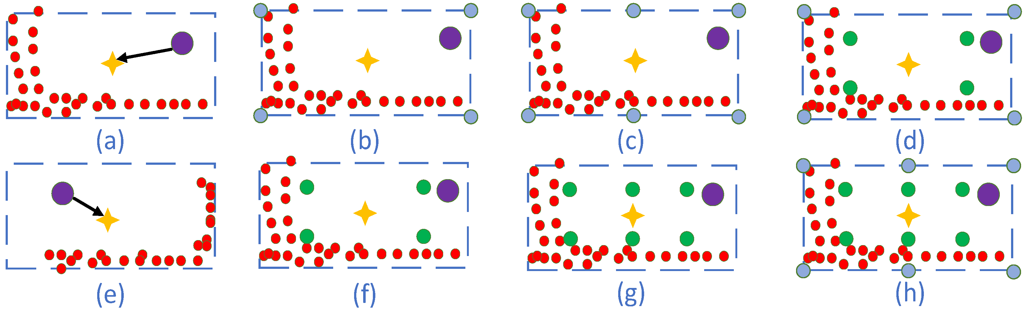
In addition, most 3D object detection methods adopt a predefined single anchor point to calculate object confidence scores. However, in such cases, the location is independent from training and no close ties can be established with the predicted bounding box. Especially, two drawbacks will appear: (1) Although the predefined anchor point position is fixed, the position of the predicted bounding boxes relative to the anchor point is shifted. In
Figure 1a, the anchor point (purple circle) stands on the top right of the predicted bounding box, while in
Figure 1e, it is on the top left of the predicted bounding box. It can be observed that the relative position of the predefined anchor points to the bounding box is uncertain. In other words, it is necessary to establish an explicit mapping correspondence between the detection object and sampling points; (2) The position of the LIDAR scanning on the object is different due to the position and orientation of the detection object. In
Figure 1a, the scan point lies in the lower left part of the bounding box, while in
Figure 1e, it is in the lower right part of the bounding box. Obviously, the traditional 3D object detection method using a single anchor point feature cannot adequately describe the whole bounding box feature. Therefore, more robust bounding box representation needs to be explored.
Considering the above problem, we proposed a KAM (keypoint-aware module) which can directly utilize the boundary keypoints from each boundary and inner keypoints by mapping the predicted real geometries to a feature map. In this way, the predicted scores can be jointly optimized with the features corresponding to the prediction bounding boxes.
In the paper, we divide the bounding box into two parts, so as to extract the sampling keypoints: the boundary parts and the inner parts. For the extraction of sampling points, three aspects are considered: (1) The contribution of the boundary points or inner points, respectively, to the 3D object detection; (2) Different sampling strategies for boundary points and inner points. For boundary keypoints sampling, two sampling strategies are adopted. One is to use only the four corner points (blue circles), as in
Figure 1b. The other is to sample the boundary uniformly. For example, as seen in
Figure 1c, three points are sampled uniformly for the boundary. For inner keypoints sampling, the points are divided into different numbers of uniform spatial grids. For example, in
Figure 1f, the BEV of the bounding box is divided into four parts, while in
Figure 1g, the BEV of the bounding box is divided into six parts; (3) A combination of boundary keypoints and inner points. The combination of different numbers of boundary and inner keypoints could improve the performance of 3D object detection differently. For example, in
Figure 1d, four samples are extracted from the boundary and other four from the inner. In
Figure 1h, the boundary parts extract six samples and the inner parts extract six samples. The combination that yields the best detection performance should be chosen.
In summary, the key contributions of the proposed method are as follows:
- (1)
In order to better retain and extract spatial information from LiDAR, as well as to extract effective cross-layer features, a novel lightweight location attention module named LLM is proposed, which can maintain an efficient flow of spatial information and incorporate multi-level features.
- (2)
A keypoints sample method is adopted to enhance the correlation between the predicted bounding box and scores, thus improving the performance of detection.
- (3)
Extensive experiments are conducted on the KITTI benchmark dataset, demonstrating that the proposed network attains good performance.
3. Approach
In this section, we introduce the proposed single-stage 3D object detection method. First, we present the design of full architecture. Second, we discuss the 3D feature extraction backbone module. Third, the proposed location attention module is discussed. Finally, we depict the strategies for keypoint-aware module in detail.
3.1. Framework
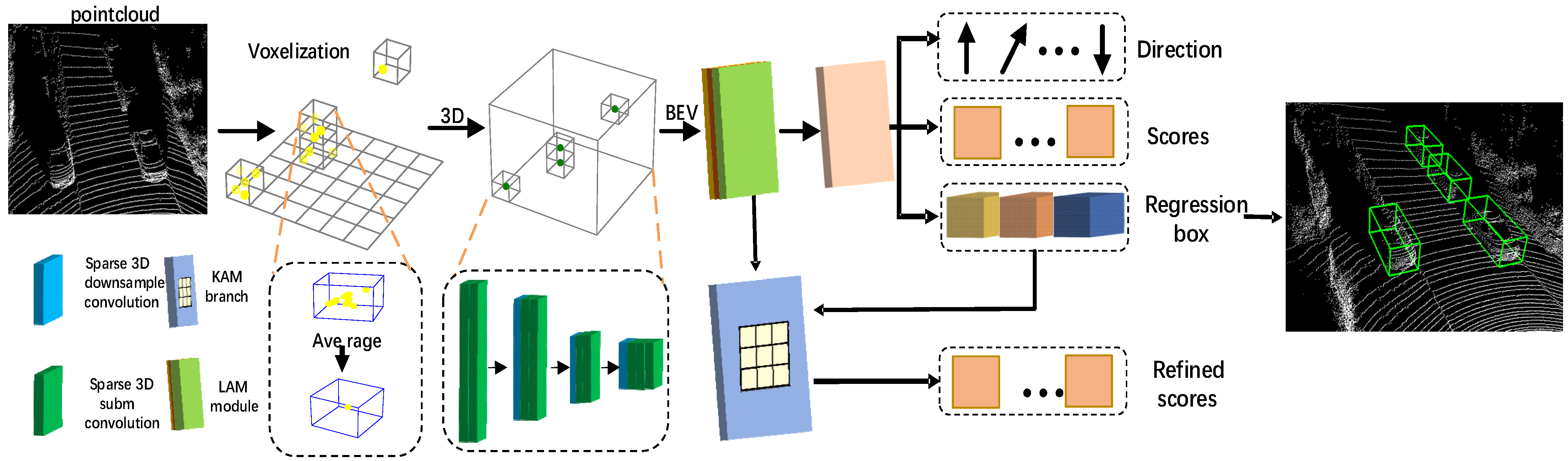
The proposed KASSD detector, as depicted in
Figure 2, consists of four components: (1) A voxel-based feature extractor; (2) A 3D backbone module; (3) A lightweight location attention module; (4) A keypoint-aware module.
The 3D backbone module voxelizes raw 3D point cloud data and converts these data to 3D sparse CNN features. Then, 3D sparse convolution is used to extract features effectively. Compared to the 3D sparse convolution, 2D convolution is more compact and efficient [
25]. Thus, the 3D sparse feature is reshaped to deliver the general 2D feature presentation. The extracted feature information contained in the point cloud is not only in higher sparsity but also substantially varies according to distances. To efficiently learn multi-layer features, a lightweight location attention module is proposed to address this problem. For pixel-wise features, most research uses one point to predict the class scores that are not adequate, thus leading to lower accuracy. By discussing different mapping feature extraction methods with influence on the results, this study proposes a novel keypoint-aware sample module. Experiments show that the novel method based on mapping is an effective way to learn the remote range and sparsity feature.
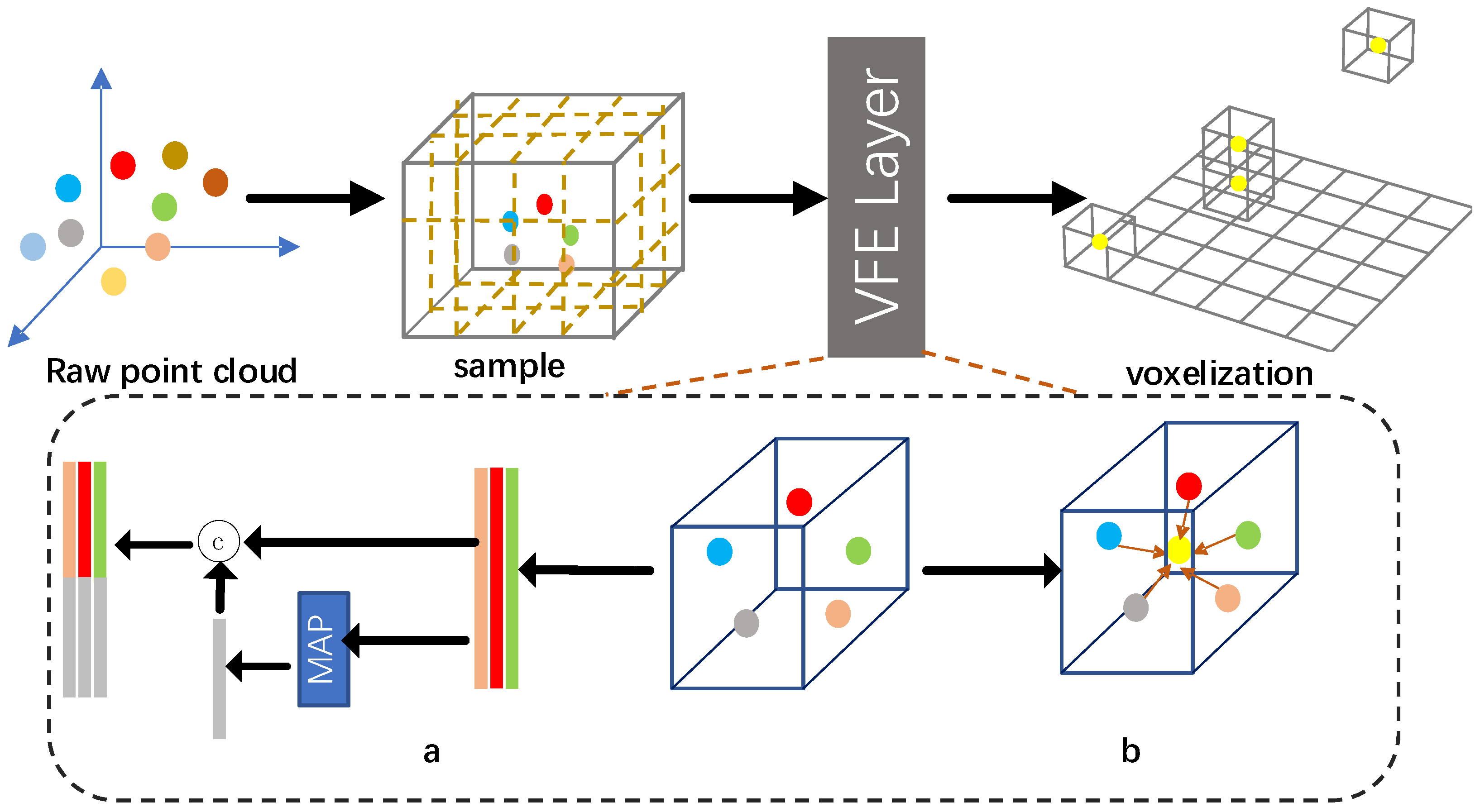
3.2. Voxelization
As we all know, the point cloud is unordered and diverse in 3D space; thus, it is necessary that the point cloud is split to heterogeneous small voxels with a resolution of dx, dy, dz, supposing that the range of point cloud is along the X, Y, Z axis. The original point cloud is equally discretized to grid cells with coordinates. Next, it is necessary to make the inter-cell point cloud uniformly. As shown in
Figure 3, there exist two methods. Shown in
Figure 3a, many papers [
26,
27] use this method to extract voxel feature, which consists of the FCN layer, pool layer, and feature concatenation layer. It is comparatively complex and consumes some time. In
Figure 3b, another method is shown, which is much more simple, and can immediately compute the mean value of all points in a specific grid excluding for empty cell.
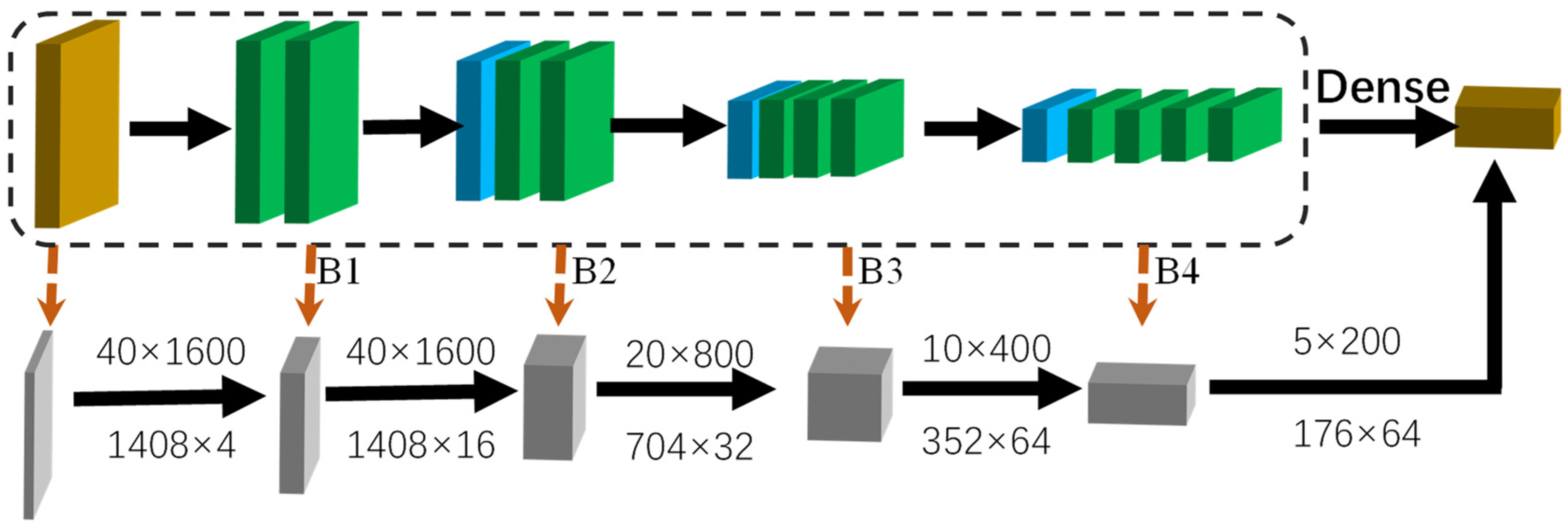
3.3. D Backbone Module
We use the popular 3D backbone module [
28] that consists of four blocks, denoted as
. Each of the blocks is serially connected to the last block. The detailed architecture is shown in
Figure 4. Blue layer means submanifold sparse convolutions layer. Green layer means general convolution. Specifically, the input features enter four blocks sequentially, and each one is shown in
Figure 4. As a result, these are four stages, where each one has a resolution of with respect to the input feature.
3.4. Lightweight Location Attention Module
Aiming to better use the feature representation of point clouds in 2D space with shallow CNN, we introduce the LLA module. Current object detectors mostly use CNN blocks or immediately use multi-level features for feature fusion to strengthen features, which cannot take full advantage of the representation potential of feature fusion. This is because shallow information is obtained through less convolution and lacks rich semantic features, while deep feature lacks excessive spatial detail [
29]. However, in the later experiments, we found that the technology which is practical in the imaging field does not scale well in the LIDAR field. Thus, we should exploit a new architecture that can extend the ability of 2D CNN to the point cloud domain.
In the experiments later, we also migrate a large CNN, of which the network depth has also been deepened. In addition, the high-level feature focuses on abstract semantic and provides the rough positions information, while the low-level feature determines the accurate object information. Thus, multi-level feature fusion should consider the importance of space and semantics of different positions in multi-level features.
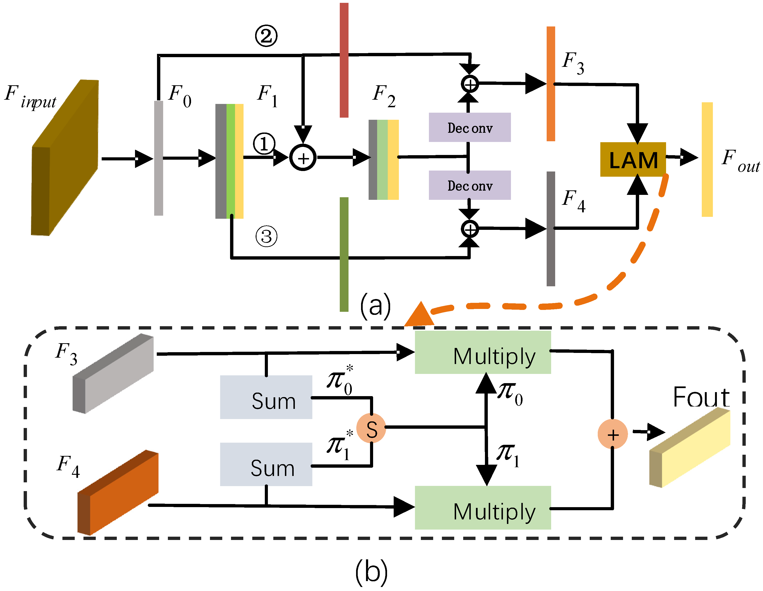
For spatial information that decreases with increasing network depth, we use a simple but effective method to maintain the efficient flow of spatial information in CNN. The detailed process is shown in
Figure 5a. We exploit the potential ability through feature reuse strategy (FRS), yielding representational power from the network.
In
Figure 5a, the proposed FRS is mainly implemented in three branches. Firstly, in branch 1, the BEV feature
is obtained by reducing input feature channels so that they can be directly summed with the following high-level feature. Secondly, the spatial feature
is obtained by using three convolutions and does not change the feature dimension. Then, the semantic feature
is obtained by one-layer convolution with stride = 2 and two-layer convolution with stride = 1 to get more abstract semantic representation. Thus, the resolution of
is reduced by half, but the number of channels doubles. To reduce the loss of spatial information, we add two branches. Branch 2 passes feature
to each of the subsequent layers. In branch 3, the intermediate layer feature
also directly passes to the subsequent feature map.
is reshaped to the original dimension by two deconvolutions so that it can be easily operated with the original feature. In other words, one branch combines the bottom layer feature, which promotes the flow of spatial information, while another branch combines the intermediate feature, which extracts rich semantic features. In addition, we combine features through sum operations. The aim is to reduce the number of parameters; it has been found that this works rather robustly in our experiments. In this way, all features are utilized multiple times.
For the sake of better incorporating multi-level features, we introduce the location attention module (LAM). Generally, the more parameters, the more difficult the training, and this will reduce the speed of inference. Different from AttaNet [
29], our module does not introduce any convolution operations, and therefore, reduces the number of parameters. In
Figure 5b, the architecture of the SSA module is illustrated in detail.
where
means element summation operation of feature map,
means the SoftMax function, and
is the attention map of the input features
and
, respectively.
The input feature of the LAM module consists of a high-level feature
and a low-level feature
corresponding to parts in
Figure 5b. First, in Equation (1), by
operation, which means element summation, we reduce the feature channel to one by adding values along channel dimension, getting a feature map feature map
and
. Next, we use the SoftMax operation to calculate relative attention mask between multi-level feature map which output two BEV attention maps,
. We can view the attention mask as an important weight distribution for each element in the feature. The higher the scores, the more important the position. Finally, since the dimension of the attention map
is the same as the input feature
and
, except for the channel dimension, we multiply the input feature by attention map directly. In Equation (2), our adaptive weighted result is calculated as follows:
The final output feature map is fed into the KAM module for the object detection task.
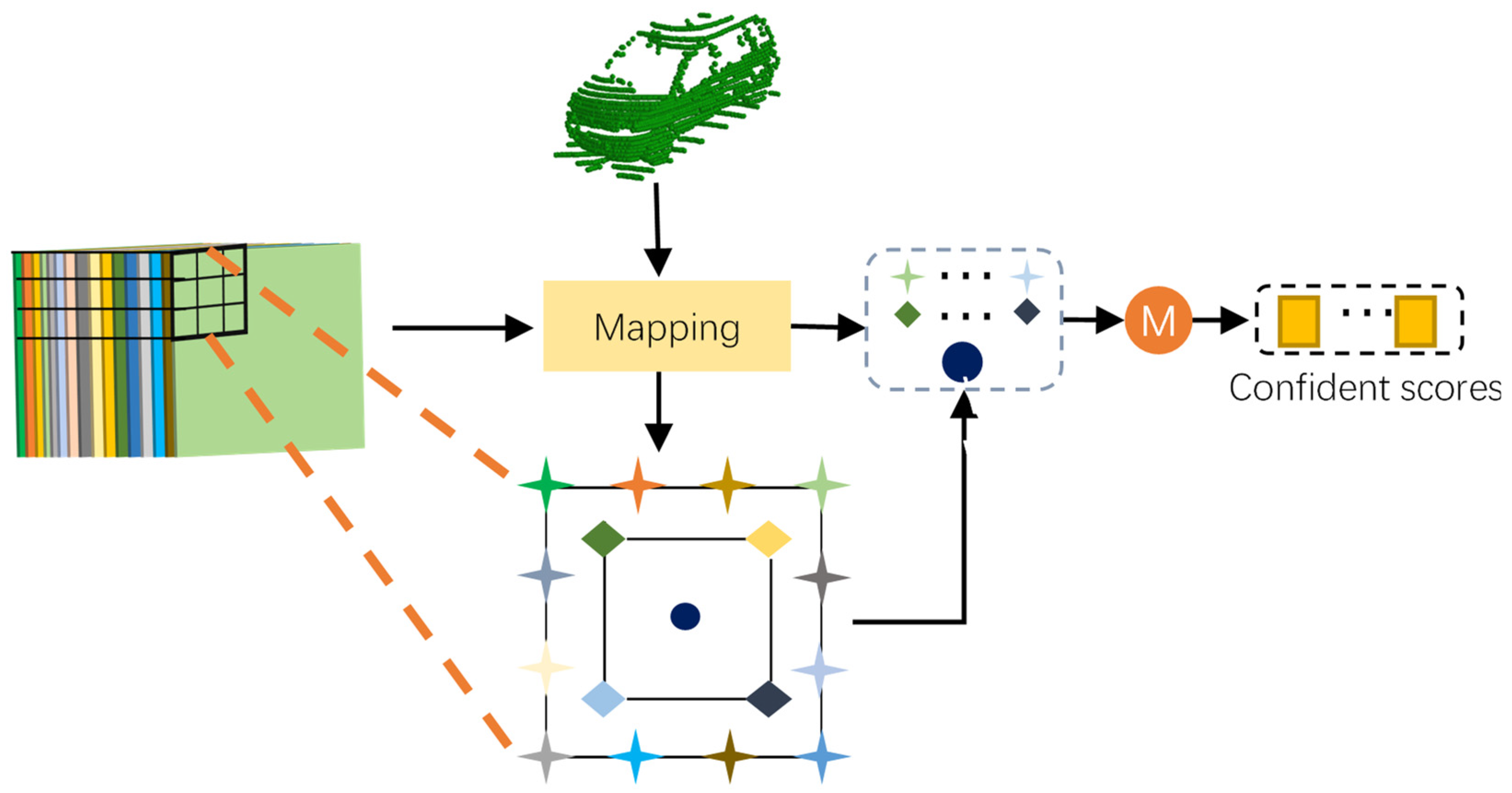
3.5. Keypoint-Aware Module
The purpose of this module is to make full use of the feature information provided by the predicted bounding box. Traditional methods use a single point to represent the proposal, ignoring geometric information and internal feature clues of the entire bounding box.
Most of the point clouds are located on the boundary of the object, which indicates that boundary features are discriminative to the object. In addition, internal features are also essential to the representation of the bounding box, which provides the abstract semantic feature of the object. However, extracting features from the entire region increases the computational burden. Inspired by the R-fcn [
30], we devise an effective proposal feature extraction method.
Thus, we introduce a keypoint-aware module (KAM) for the score prediction. The structure of KAM is shown in detail in
Figure 6. To generate effective feature representation for each prediction box in the current training process, the KAM module uses the features at the boundary (star) and inner area (diamond and central circle) sampling points to represent the bounding box. It can capture rich semantic features of the whole object and establish explicit location-feature map relation, which is essential to alleviate the misalignment problem between scores and the prediction bounding box. Specifically, we divide the object detection scores into two parts: a boundary-aware module and an inner-aware module.
The KAM module takes the last layer feature map as the input and consists of three convolutions to output the confident map.
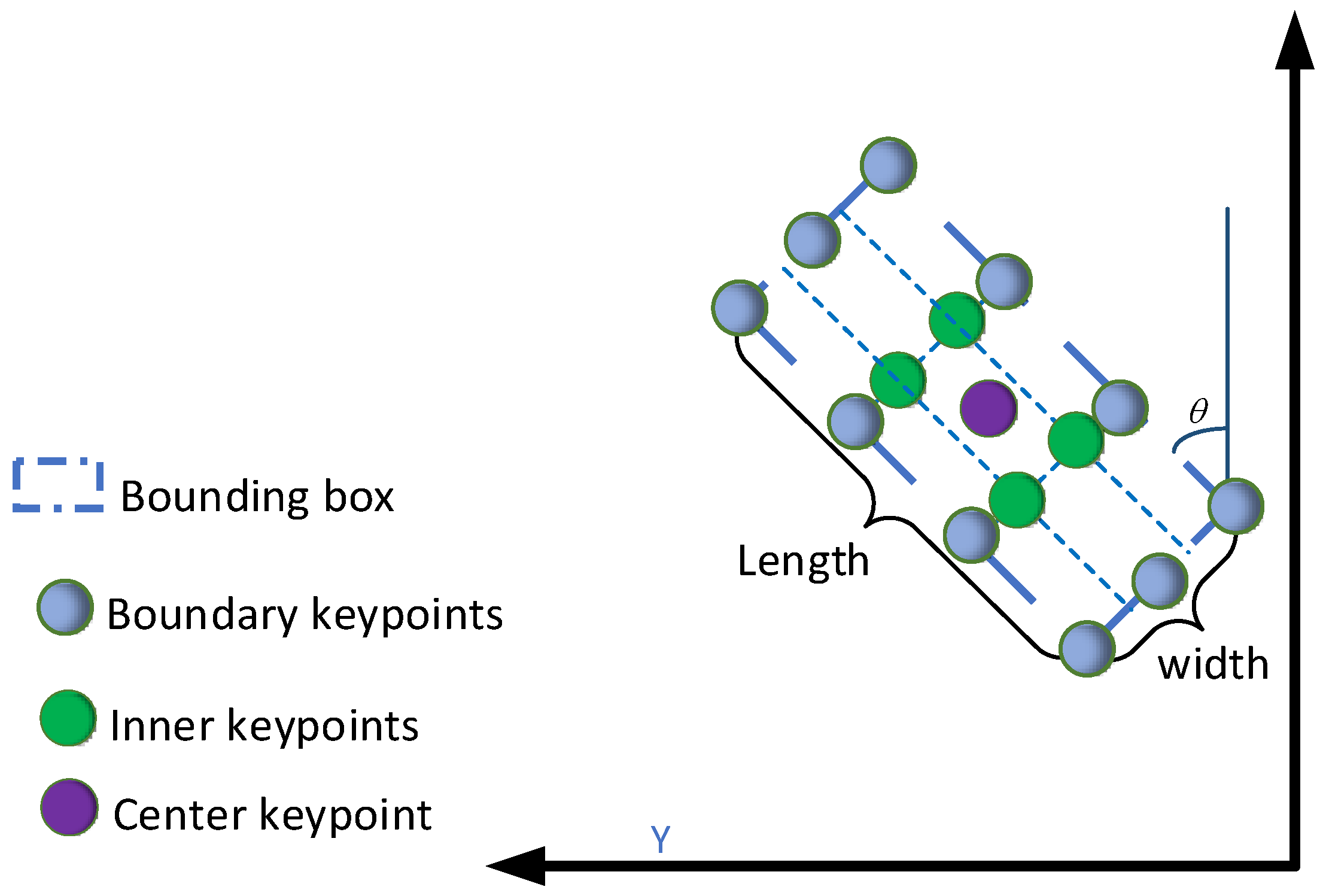
To the boundary area, our boundary-aware module selects representative features using uniform sampling, such as the blue circle in
Figure 7. Specifically, long edges are represented by m points and short edges by n points. Since the labeled boxes are rectangular, the number of keypoints on opposite sides is the same. Given the proposal bounding box from the regression branch, subscript i indicates the i-th point along the
x-axis and subscript j indicates the j-th point along the
y-axis.
is the center location coordinate of the bounding box, represented by the purple circle in
Figure 7. Lastly,
are the width, length, and angle.
The above values are in the LiDAR coordinate system. Moreover, the boundary keypoints calculation method can be defined as follows:
where
are a set of keypoints linearly spaced between
. In
Figure 7, for example, the long edge is represented by four keypoints,
. Moreover, the wide edge is represented by three keypoints,
. Lastly,
, and
denote the left, right, bottom, and top edges, respectively.
Given a certain area inside a bounding box, the inner-aware module divides the inner area evenly into the grid, using grid vertices as feature points. In addition, the calculation method is similar to the boundary points.
If the proposed box is represented by a total of K keypoints, then the corresponding final convolution outputs the K-layer feature map on the so-called score map. Each score map describes the feature response for keypoints of the predicted bounding box. For example, the first scores map represents the score of the top-left point. Assuming the input feature maps are in the order of (left border, top border, right border and bottom border, inner point), each feature point score
F can be formulated with the following equation:
where
denotes the total number of inner points.
.
is a uniform representation for mapped coordinates of the keypoint.
represents real-world coordinates; moreover,
.
x,
y are the coordinates with respect to the LiDAR coordinate system. Typically,
is fractional; thus, the
value is calculated by bilinear interpolation
with the adjacent position.
signifies the coordinates offset and scale,
.
are the coordinates with respect to the feature map. The mean value of all keypoints is calculated as final scores.
3.6. Loss Function
The loss function of our work is a combination of the Regression loss function, class loss function, direction loss function, and keypoints loss function. For the bounding box, the parameterizations of seven coordinates are employed, as in [
21]:
where
. The box’s center coordinates and its width, length, height, and angle are, respectively, denoted as
. Parameters
and
are for the predicted box, ground truth box, and anchor box, respectively. Likewise,
.
One-stage 3D object detection faces an extreme imbalance during training. Thus, we commonly use focal loss [
31] to deal with this problem by assigning well-classified examples with lower weights:
For box regression,
loss is adopted, as shown as follows:
Thus, the box loss can be defined as:
where
indicate the predicted encoded value and ground truth encoded value in Formula (1), respectively.
We use the discrete approach by introducing sin function and direction classifier cross-entropy.
Hence, the multi-task loss function of our KASSD for end-to-end training is calculated as follows:
where
are hyper-parameters that weight each loss term of multi-task learning.
4. Experiments
4.1. Dataset and Evaluation Metrics
We comprehensively conduct experiments on the KITTI dataset [
32], a large-scale dataset for LiDAR point-cloud object detection. The dataset contains 7481 training samples and 7518 test samples. Following previous work [
13,
26,
33] the training samples are split into a training set consisting of 3712 samples and a validation set consisting of 3769 samples, which is about a 1:1 ratio.
Furthermore, the KITTI datasets have three levels: easy, moderate, and hard, which depend on the size, occlusion, and truncation levels. To facilitate comparison with previous work, we use the car category and calculate the average precision (AP) to evaluate the result for different difficulty levels.
AP is the common evaluation metric for 3D object detection in the KITTI. Specifically, the
AP summaries the shape of the precision/recall curve, and is defined as the mean precision at a set of equally spaced recall levels. In KITTI, 41 recall positions are official evaluation protocol. For example,
is calculated according to the following equation:
where
is a set of 11 recall values linearly spaced between [0, 1].
Following the metrics used in the previous paper, we calculate AP with 11 recall positions to evaluate the validation set.
In addition, practical application of research is one of the important criteria for judging work. Thus, we establish a dataset of 3D object detection for our school scene named the WHUT dataset. Our dataset contains 2000 frames of samples, annotated over one month. Furthermore, we use 1500 frames for training and 500 frames for validation. Moreover, we adopt the same metrics as KITTI without difficulty division.
4.2. Implementation Details
We use the most commonly voxelization with grid of [0.05, 0.05, 0.1] meters and crop the original point cloud in ranges [0, 70.4], [−40, 40], [−3, 1] meters along the x, y, z axes. Every point on the last layer of feature corresponds to two pre-defined boxes, which have the same size (width = 1.6 m, length = 3.9 m, height = 1.56 m) and different orientations (0° and 90°).
The network is trained by Adaptive Moment Estimation (Adam) [
34] with the cosine annealing learning rate. In addition, our model is trained for 80 epochs with a batch size of two on four 2080Ti GPU cards. In the experiments, we set
to 2, 1, 1, and 0.2, respectively.
4.3. Evaluation with the KITTI Dataset
We evaluate the performance of our KASSD with the KITTI dataset by submitting the detection results to the KITTI server for evaluation. As shown in
Table 1, our proposed method outperforms most existing methods, such as 3DSSD, DVFENet, SECOND, STD, PointRCNN, and TANet, by roughly 0.04 to 3.0 points, but is slightly inferior to 3D-SSD on hard
AP. The performance of KASSD in the validation set of the car category is shown in
Table 2.
From the results, it can be observed that our method outperforms several other methods across all difficulty levels. Our method performance outperforms other methods on moderate and hard levels. The lack of labeling on the distant and heavily occluded object is the primary difference in cause. In some cases, despite the fact that the network learns features, the object detected in certain situations is deemed to be incorrect. Another cause is the dataset’s inconsistent distribution, as mentioned in CIA-SSD [
10]. In addition, 3D IoU-Net [
8] uses a single point to predict IOU, whereas our approach employs richer regional information to increase the network’s ability to estimate the confidence scores of the bounding box. In
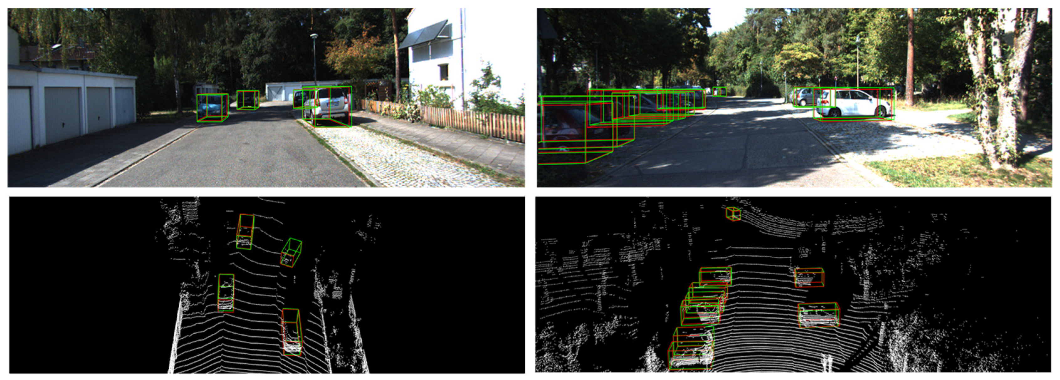
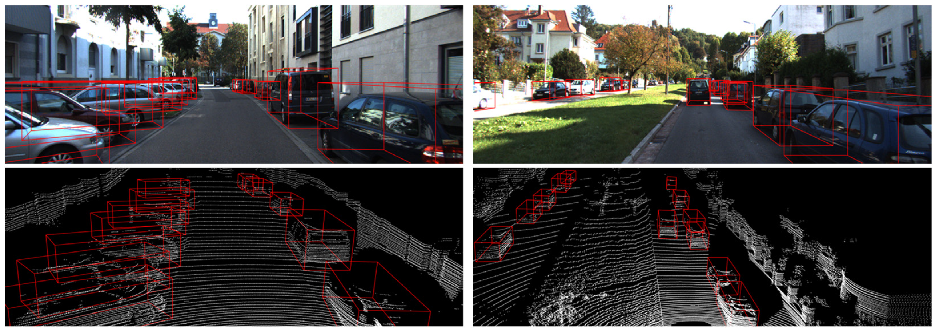
Table 1, it is obvious that our method achieves better performance. We also show some qualitative result of validation and test sets in
Figure 8 and
Figure 9, respectively.
4.4. Evaluation on the WHUT Dataset
We show the performance of our model and SECOND in
Table 3 and compare their
AP. In addition, the WHUT dataset is recorded by 32-beam LiDAR, which has a lower resolution than the 64-beam LiDAR utilized by KITTI. However, our model still outperforms SECOND 0.97
AP. It demonstrates that our proposed KASSD object detector is still effective in low-resolution LiDAR.
4.5. Ablation Study
To demonstrate the effectiveness of the proposed module, we compare the proposed KASSD to a baseline detector.
Table 4 presents the results of
AP with algorithms equipped with various submodules. First, we investigate the effect of LLM by substituting the proposed module for the convolution component. Compared with the baseline, easy, moderate, and hard
AP are 0.32, 0.4, and 0.27 higher than the baseline, respectively, demonstrating that the LLM module better retains spatial information and fuses high-resolution and sematic features to concentrate more on discriminative information. We further conduct experiments on KAM. The validation results show that the proposed module significantly outperforms the baseline methods with 0.85, 0.89, and 1.21 on all difficulty levels. Moreover, our proposed method outperforms baseline model by 1.05, 1.11, and 1.24, especially when all submodules are combined.
To further highlight the performance of the LLM relative to other feature extraction modules, we compare it with other advanced approaches in
Table 5. TANet [
33] is a new feature fusion method that has been proposed recently, using pyramid modules. Moreover, we replaced the LLM modules with PSA modules for training. The result shows that the PSA improves the
AP significantly on the easy level. However, for the moderate and hard levels, the
AP value drops over 0.3. This is proof that our method has more powerful spatial and semantic information extraction capabilities compared to other advanced methods.
We also exploit the impact of the receptive field to verify the suitability of traditional enhancement techniques in point clouds. The astrous convolution is an effective method for enlarging the receptive field and play an important role in object detection. Thus, we insert SPP [
45] and DENSEASPP [
46] separately into the intermediate convolution layer to test the effect of receptive field. We can find that the
AP in each difficulty level drops dramatically. In other words, a direct increase in the receptive field using astrous convolution does not contribute to the performance, which also validates the difference between sparse point clouds and dense image features.
In
Table 6, we delve into the representational power of various parts of the bounding box and different numbers of sampling points. Firstly, we analyze the effect of the four boundary corner points, which enhance the easy, moderate, and hard
AP by 0.33, 0.35, and 0.48, respectively. In addition, experiments on the increase of boundary points were also conducted. The detection performance was improved again when the number of boundary points was increased to 18; the easy, moderate, and hard
AP was increased by 0.23, 0.15, and 0.16. However, when the number of boundary points was increased to 28, the easy and moderate
AP dropped slightly. Based on the results of the proceeding experiments, it is clear that the representation capability of the predicted bounding box is improved by increasing the number of keypoints.
Next, we examine the best performance in the case of using inner keypoints. We divide the internal area evenly into grids and take joints as keypoints for sampling. Following the previous convention of the score, we still add predefined anchor points as one of the sampling points. As a result, we were able to obtain 11 keypoints. For the inner points, we observe a huge AP improvement of 0.8, 0.81, and 0.78 for easy, moderate, and hard levels, demonstrating the importance of describing the inner area for an object representation method.
Table 6 further shows how employing a variety of sampling points over the entire area improves the
AP. We combine the sampling of the inner keypoints with the boundary keypoints and call it mixed keypoints sampling. Compared to boundary keypoints (Row 3), mixed keypoints sampling outperforms it by 0.29, 0.39, and 0.51
AP on the easy, moderate, and difficult levels. To inner keypoints (Row 5), mixed keypoints sampling brings an improvement of 0.37 on the hard level of difficulty. This indicates that mixed keypoints sampling achieves higher performance than sampling with only boundary or internal key-points. Thus, we are able to conclude that boundary keypoints and inner keypoints can complement each other to improve the performance of 3D object detector.
In addition, we note that varying the number of keypoints sampling has an impact on the results. In Row 7, we can find that performance degrades when too many mixed keypoints sampling are extracted.
4.6. Runtime Analysis
Running speed, particularly in autonomous driving, plays an important role in object detection. Furthermore, the speed of inference fluctuates in a small range. Thus, all runtimes were averaged from ten runs of the algorithm.
The average inference time of our method is 45.9 ms. The inference time is calculated as follows. The point cloud must first be loaded and preprocessed (2.3 ms). The data tensor is then processed by KASSD (42.9 ms). Moreover, post-processing was done to get the final result (0.7 ms). Because real-time detection is critical in autonomous driving, we examine the detection speeds of several approaches. In
Table 7, we can find that our proposed KASSD is 597.1 ms, 14.1 ms, and 0.4 ms faster than point-GNN, Associate-3Ddet, and SECOND, respectively. Compared with 3DSSD, the inference speed of our model is slightly slower. However, our model outperforms 3DSSD by 0.43, 0.89, and 0.24
AP on easy, moderate, and hard levels of difficulty, respectively. In other words, KASSD improves the 3D object detection performance with tolerable computation overhead.
4.7. Discussion
We proposed a simple keypoint-aware module for 3D object detection, which has four advantages. Firstly, our proposed KAM (keypoint-aware module) solves the problem that the relative position of the predefined anchor point and predicted bounding box is uncertain in the traditional 3D single-stage object detection. Secondly, experimental results show that both boundary and inner points can improve the performance of the 3D object detector. This also illustrates that the predefined anchor points of conventional 3D object detectors lack sufficient information, which may lead to a decrease in performance. Thirdly, the ideal option is to use sampling of a mix of keypoints. It indicates that inner keypoints and boundary keypoints adequately capture the context of the predicted bounding box and effectively produce high-quality object description. Finally, our proposed method achieves competitive performance.
However, there are some limits to our method. Our proposed method uses a fixed keypoints sampling mechanism for all predicted objects and cannot adaptively select the best keypoints. It may impede the ability of the 3D object detectors to perform well. In the future, we will focus on a learnable keypoint-aware module, which may result in more significant improvements.


