


Virtual Axle Detector Based on Analysis of Bridge Acceleration Measurements by Fully Convolutional Network
 , , , , , and
Abstract
:1. Introduction
2. Methods
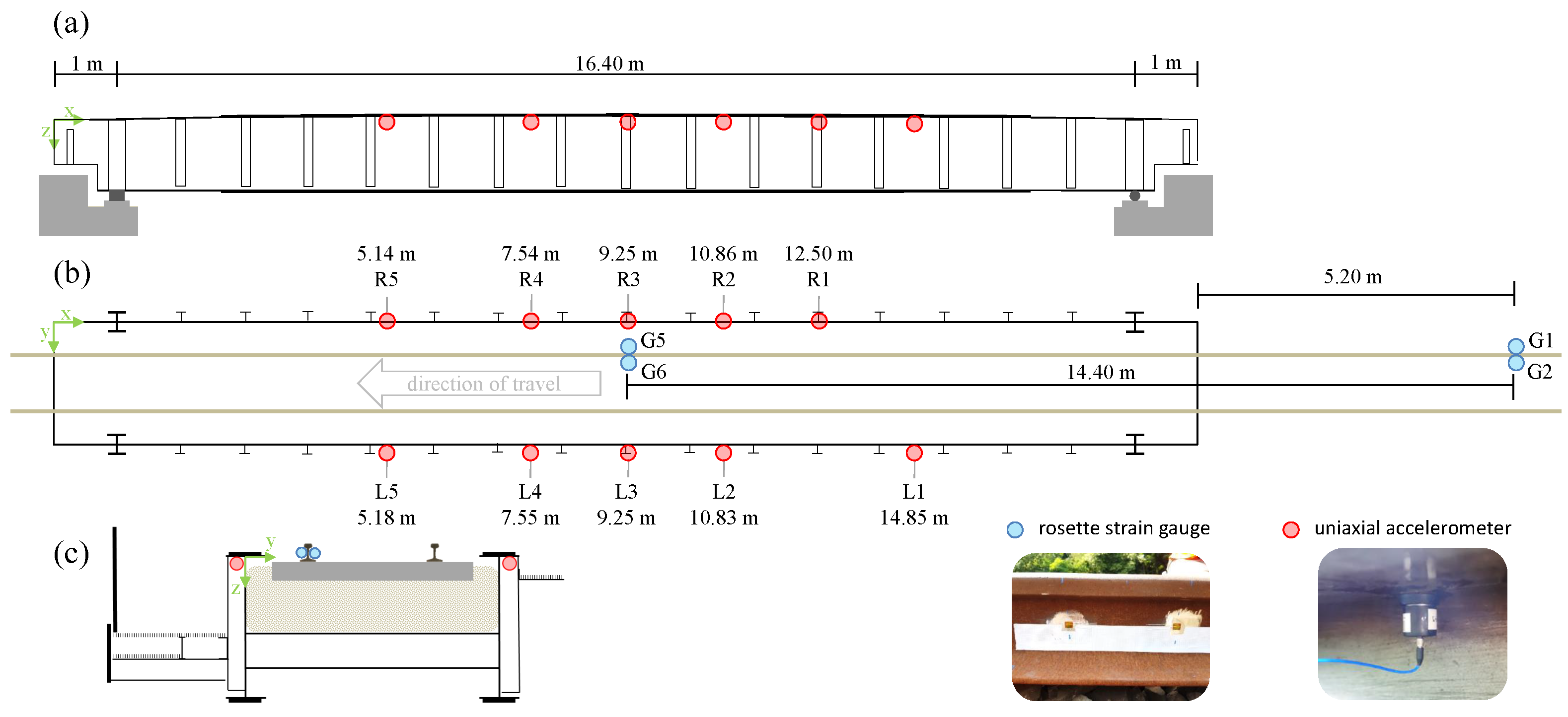
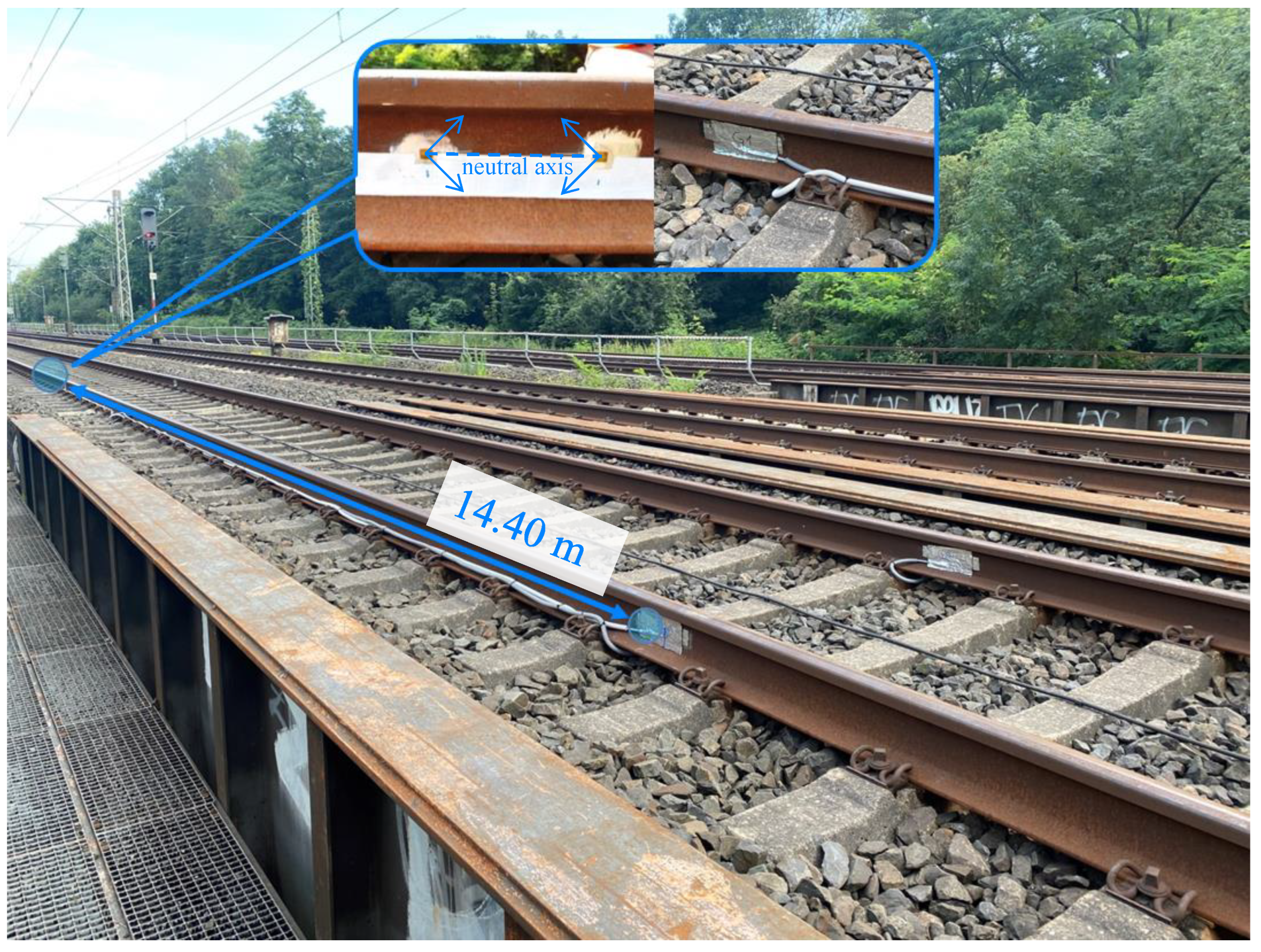
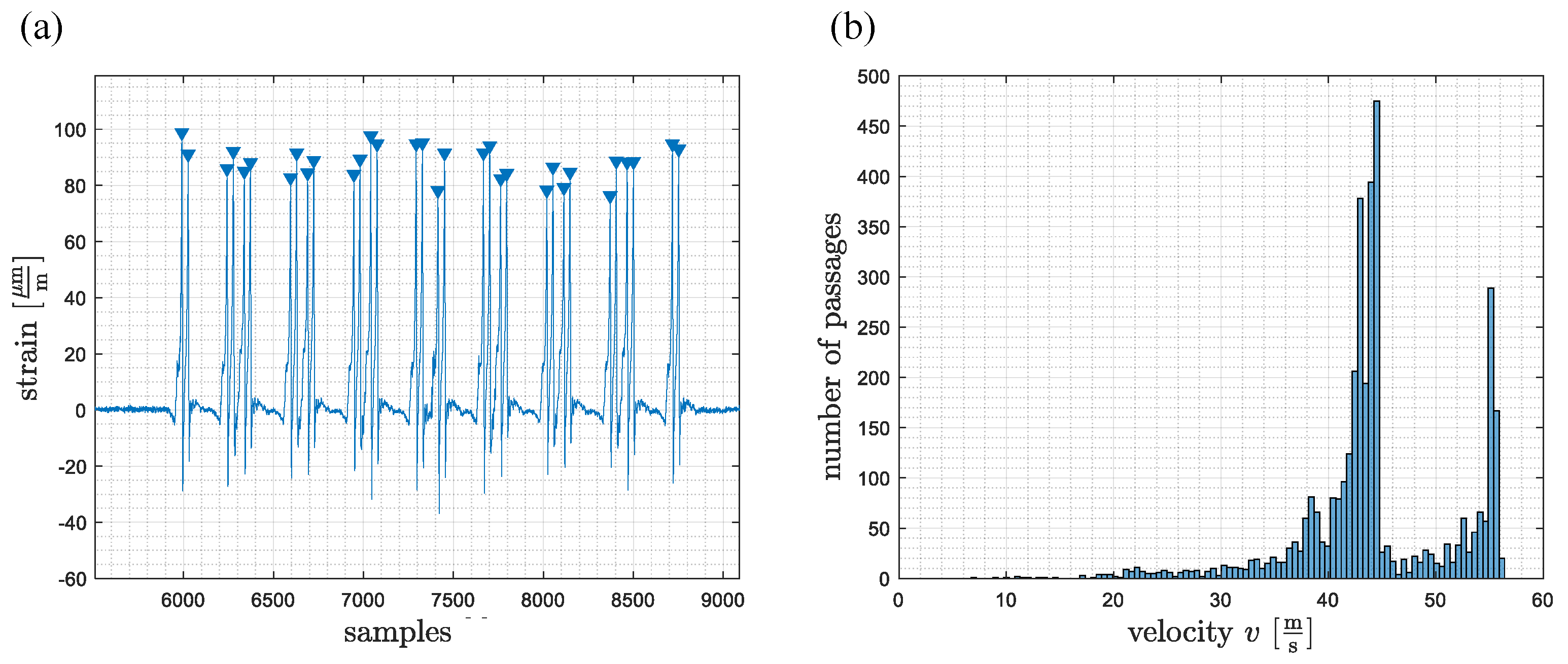
2.1. Data Acquisition
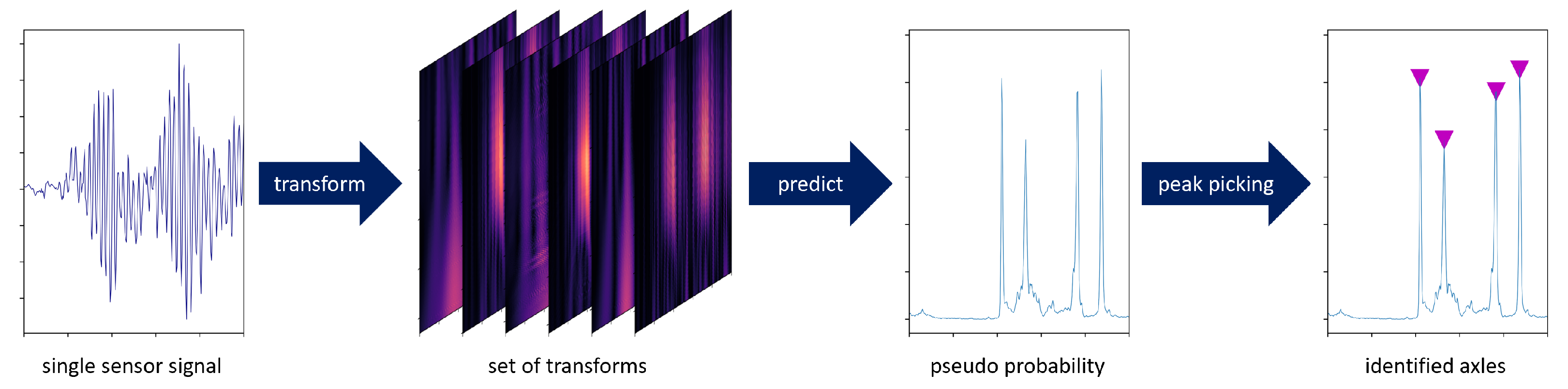
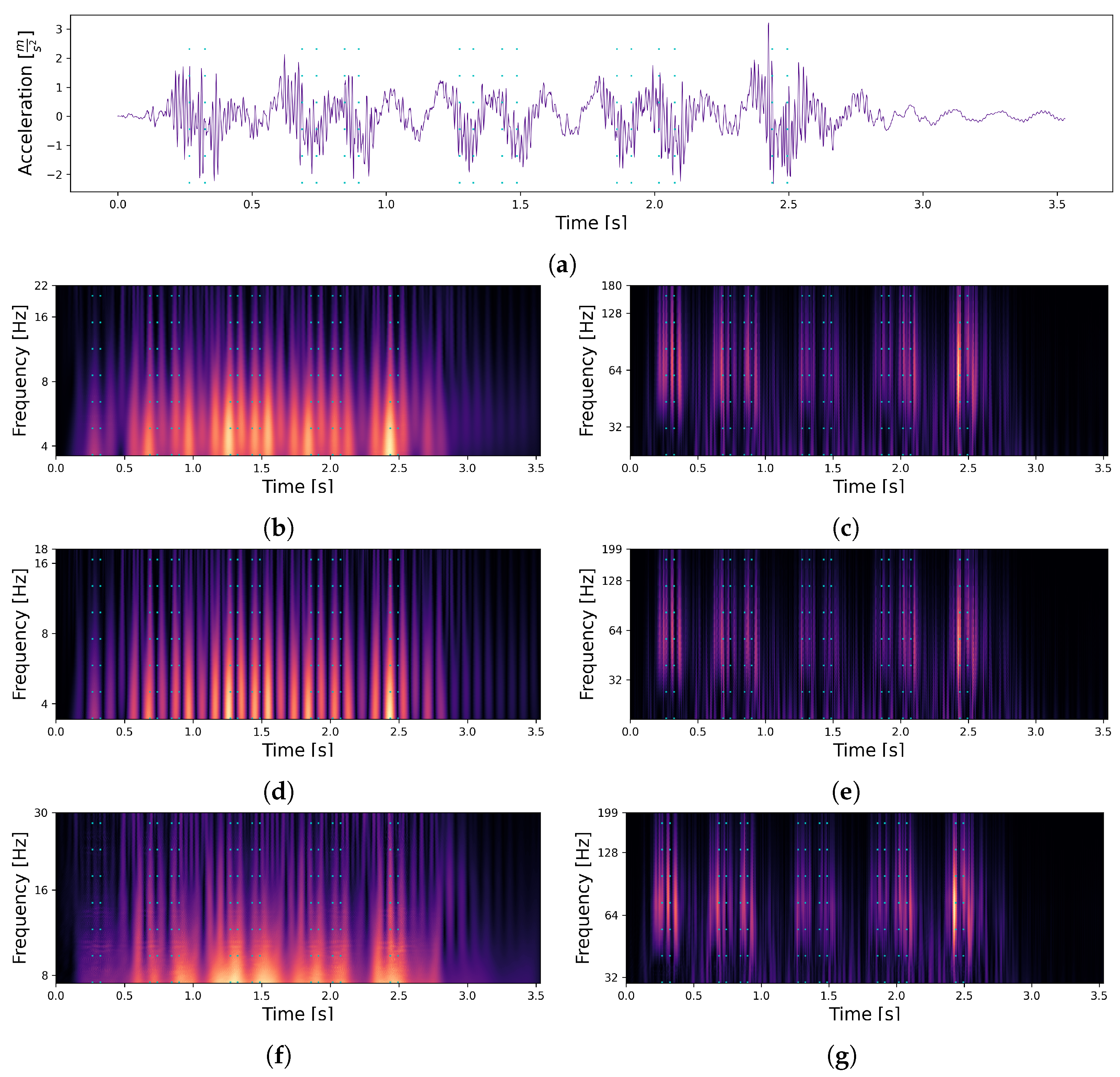
2.2. Data Transformation
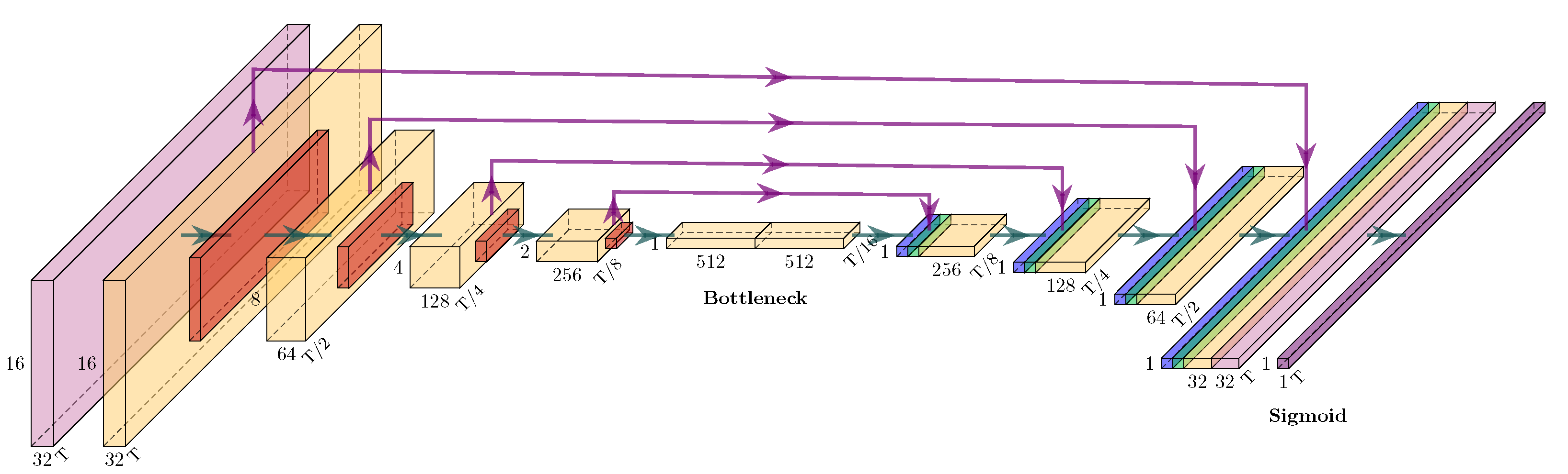
2.3. Model Definition
2.4. Loss Function
2.5. Evaluation Metrics
2.6. Optimization of
3. Results and Discussion
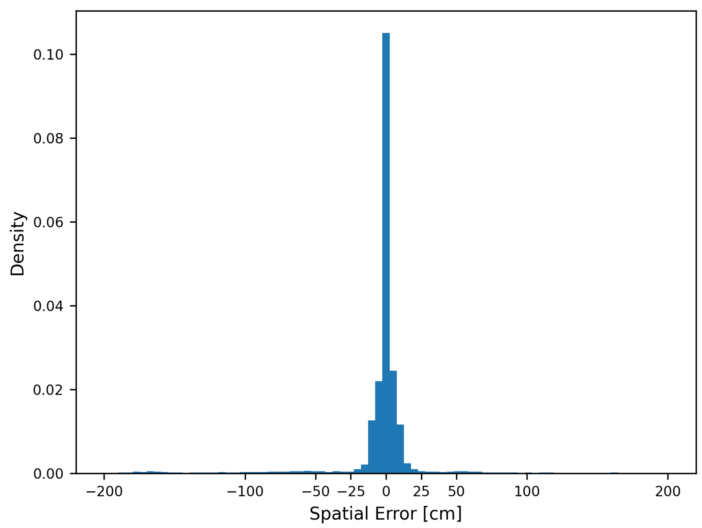
- 200 cm as the minimum wheel distance;
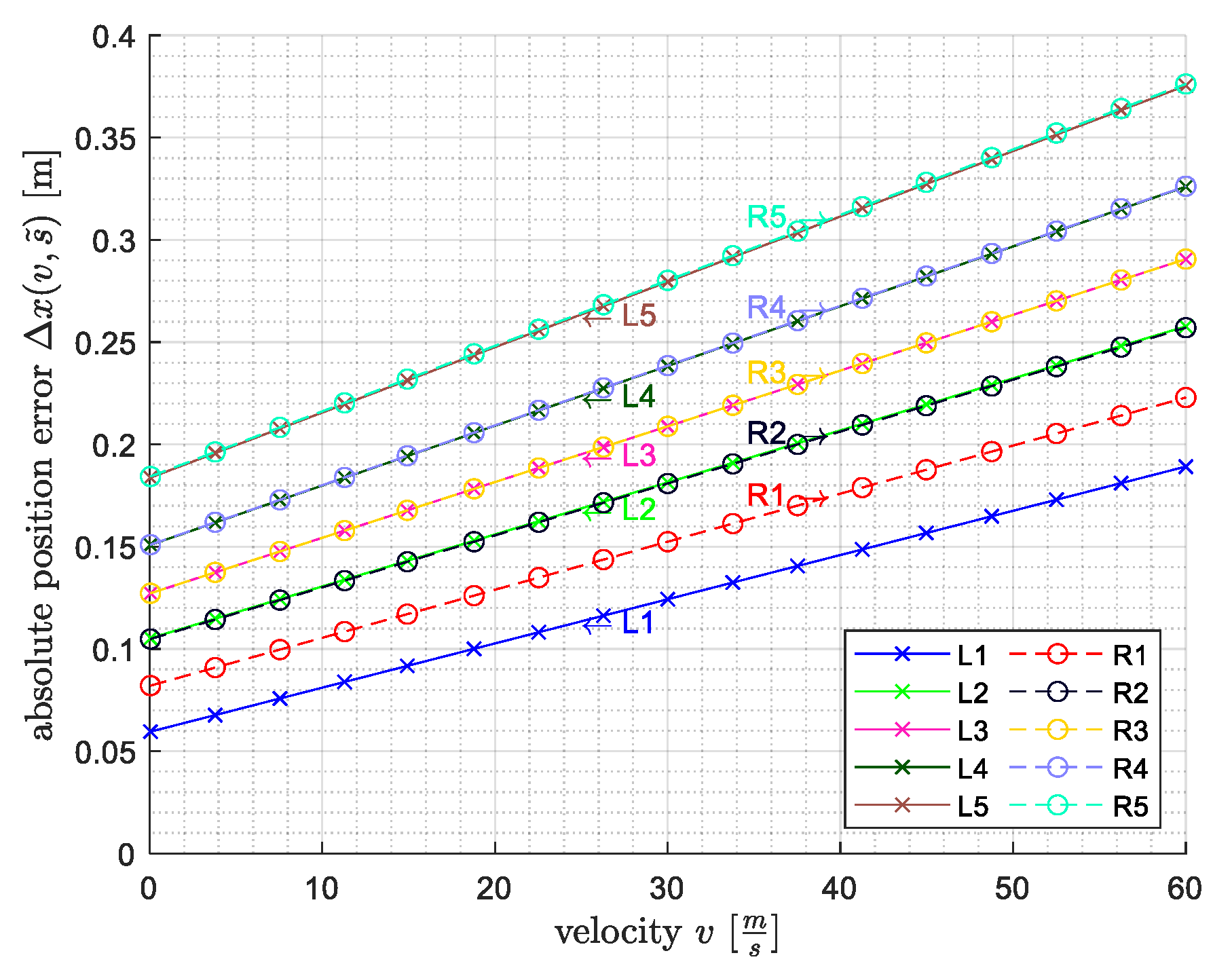
- 37 cm as the maximum labelling error (Figure 6);
- 20 cm as the length of the wheel load measuring point.
4. Conclusions
Author Contributions
Funding
Data Availability Statement
Conflicts of Interest
Abbreviations
| BWIM | Bridge Weigh-In-Motion |
| CB | Convolution block |
| CE | Cross Entropy |
| CNN | Convolutional Neural Network |
| CWT | Continuous-Wavelet-Transformation |
| DGPS | Differential Global Positioning System |
| FAD | Free-of-axle-detector |
| FCN | Fully Convolutional Network |
| FL | Focal Loss |
| NOR | Nothing-on-road |
| RB | Residual block |
| ReLU | Rectified Linear Unit |
| SHM | Structural health monitoring |
| STFT | Short Time Fourier Transformation |
| VAD | Virtual Axle Detector |
References
- ASCE. Structurally Deficient Bridges | Bridge Infrastructure | ASCE’s 2021 Infrastructure Report Card. 2021. Available online: https://infrastructurereportcard.org/cat-item/bridges-infrastructure/ (accessed on 28 June 2022).
- Geißler, K. Front Matter; John Wiley & Sons, Ltd.: Hoboken, NJ, USA, 2014. [Google Scholar] [CrossRef]
- Knapp, N. Brücken bei der Deutschen Bahn. 2019. Available online: https://www.deutschebahn.com/de/presse/suche_Medienpakete/medienpaket_bruecken-6854340 (accessed on 28 June 2022).
- Chan, T.; Yu, L.; Law, S.; Yung, T. Moving Force Identification Studies, I: Theory. J. Sound Vib. 2001, 247, 59–76. [Google Scholar] [CrossRef]
- Kouroussis, G.; Caucheteur, C.; Kinet, D.; Alexandrou, G.; Verlinden, O.; Moeyaert, V. Review of Trackside Monitoring Solutions: From Strain Gages to Optical Fibre Sensors. Sensors 2015, 15, 20115–20139. [Google Scholar] [CrossRef] [PubMed] [Green Version]
- Firus, A.; Kemmler, R.; Berthold, H.; Lorenzen, S.; Schneider, J. A time domain method for reconstruction of pedestrian induced loads on vibrating structures. Mech. Syst. Signal Process. 2022, 171, 108887. [Google Scholar] [CrossRef]
- Kazemi Amiri, A.; Bucher, C. A procedure for in situ wind load reconstruction from structural response only based on field testing data. J. Wind. Eng. Ind. Aerodyn. 2017, 167, 75–86. [Google Scholar] [CrossRef]
- Hwang, J.; Kareem, A.; Kim, W. Estimation of modal loads using structural response. J. Sound Vib. 2009, 326, 522–539. [Google Scholar] [CrossRef]
- Lourens, E.; Papadimitriou, C.; Gillijns, S.; Reynders, E.; De Roeck, G.; Lombaert, G. Joint input-response estimation for structural systems based on reduced-order models and vibration data from a limited number of sensors. Mech. Syst. Signal Process. 2012, 29, 310–327. [Google Scholar] [CrossRef]
- Firus, A. A Contribution to Moving Force Identification in Bridge Dynamics. Ph.D. Thesis, Technische Universität, Darmstadt, Darmstadt, Germany, 2022. [Google Scholar] [CrossRef]
- Lydon, M.; Robinson, D.; Taylor, S.E.; Amato, G.; Brien, E.J.O.; Uddin, N. Improved axle detection for bridge weigh-in-motion systems using fiber optic sensors. J. Civ. Struct. Health Monit. 2017, 7, 325–332. [Google Scholar] [CrossRef] [Green Version]
- Wang, H.; Zhu, Q.; Li, J.; Mao, J.; Hu, S.; Zhao, X. Identification of moving train loads on railway bridge based on strain monitoring. Smart Struct. Syst. 2019, 23, 263–278. [Google Scholar] [CrossRef]
- Yu, Y.; Cai, C.; Deng, L. State-of-the-art review on bridge weigh-in-motion technology. Adv. Struct. Eng. 2016, 19, 1514–1530. [Google Scholar] [CrossRef]
- He, W.; Ling, T.; OBrien, E.J.; Deng, L. Virtual Axle Method for Bridge Weigh-in-Motion Systems Requiring No Axle Detector. J. Bridge Eng. 2019, 24, 04019086. [Google Scholar] [CrossRef]
- Thater, G.; Chang, P.; Schelling, D.R.; Fu, C.C. Estimation of bridge static response and vehicle weights by frequency response analysis. Can. J. Civ. Eng. 1998, 25, 631–639. [Google Scholar] [CrossRef]
- Zakharenko, M.; Frøseth, G.T.; Rönnquist, A. Train Classification Using a Weigh-in-Motion System and Associated Algorithms to Determine Fatigue Loads. Sensors 2022, 22, 1772. [Google Scholar] [CrossRef] [PubMed]
- Bernas, M.; Płaczek, B.; Korski, W.; Loska, P.; Smyła, J.; Szymała, P. A Survey and Comparison of Low-Cost Sensing Technologies for Road Traffic Monitoring. Sensors 2018, 18, 3243. [Google Scholar] [CrossRef] [PubMed] [Green Version]
- Yu, Y.; Cai, C.; Deng, L. Vehicle axle identification using wavelet analysis of bridge global responses. J. Vib. Control. 2017, 23, 2830–2840. [Google Scholar] [CrossRef]
- O’Brien, E.J.; Hajializadeh, D.; Uddin, N.; Robinson, D.; Opitz, R. Strategies for Axle Detection in Bridge Weigh-in-Motion Systems. In Proceedings of the International Conference on Weigh-In-Motion, Dallas, TX, USA, 3–7 June 2012; pp. 79–88. [Google Scholar]
- Zhao, H.; Tan, C.; OBrien, E.J.; Uddin, N.; Zhang, B. Wavelet-Based Optimum Identification of Vehicle Axles Using Bridge Measurements. Appl. Sci. 2020, 10, 7485. [Google Scholar] [CrossRef]
- Kalhori, H.; Alamdari, M.M.; Zhu, X.; Samali, B.; Mustapha, S. Non-intrusive schemes for speed and axle identification in bridge-weigh-in-motion systems. Meas. Sci. Technol. 2017, 28, 025102. [Google Scholar] [CrossRef]
- Zhu, Y.; Sekiya, H.; Okatani, T.; Yoshida, I.; Hirano, S. Acceleration-Based Deep Learning Method for Vehicle Monitoring. IEEE Sensors J. 2021, 21, 17154–17161. [Google Scholar] [CrossRef]
- Daubechies, I. The wavelet transform, time-frequency localization and signal analysis. IEEE Trans. Inf. Theory 1990, 36, 961–1005. [Google Scholar] [CrossRef]
- Chatterjee, P.; OBrien, E.; Li, Y.; González, A. Wavelet domain analysis for identification of vehicle axles from bridge measurements. Comput. Struct. 2006, 84, 1792–1801. [Google Scholar] [CrossRef] [Green Version]
- Lorenzen, S.R.; Riedel, H.; Rupp, M.; Schmeiser, L.; Berthold, H.; Firus, A.; Schneider, J. Virtual Axle Detector based on Analysis of Bridge Acceleration Measurements by Fully Convolutional Network. arXiv 2022, arXiv:2207.03758. [Google Scholar] [CrossRef]
- Brunton, S.L.; Kutz, J.N. Data-Driven Science and Engineering: Machine Learning, Dynamical Systems, and Control; Cambridge University Press: Cambridge, UK, 2019. [Google Scholar] [CrossRef] [Green Version]
- Mallat, S. A theory for multiresolution signal decomposition: The wavelet representation. IEEE Trans. Pattern Anal. Mach. Intell. 1989, 11, 674–693. [Google Scholar] [CrossRef] [Green Version]
- Lee, G.R.; Gommers, R.; Waselewski, F.; Wohlfahrt, K.; O’Leary, A. PyWavelets: A Python package for wavelet analysis. J. Open Source Softw. 2019, 4, 1237. [Google Scholar] [CrossRef]
- Long, J.; Shelhamer, E.; Darrell, T. Fully convolutional networks for semantic segmentation. In Proceedings of the 2015 IEEE Conference on Computer Vision and Pattern Recognition (CVPR), Boston, MA, USA, 7–12 June 2015; pp. 3431–3440. [Google Scholar] [CrossRef] [Green Version]
- Ronneberger, O.; Fischer, P.; Brox, T. U-Net: Convolutional Networks for Biomedical Image Segmentation. In Proceedings of the Medical Image Computing and Computer-Assisted Intervention—MICCAI 2015, Munich, Germany, 5–9 October 2015; Springer International Publishing: Cham, Switzerland, 2015; pp. 234–241. [Google Scholar] [CrossRef] [Green Version]
- Géron, A. Hands-On Machine Learning with Scikit-Learn, Keras, and TensorFlow: Concepts, Tools, and Techniques to Build Intelligent Systems; O’Reilly UK Ltd.: Sebastopol, UK, 2019; ISBN 9781492032649. [Google Scholar]
- He, K.; Zhang, X.; Ren, S.; Sun, J. Deep Residual Learning for Image Recognition. In Proceedings of the 2016 IEEE Conference on Computer Vision and Pattern Recognition (CVPR), Las Vegas, NV, USA, 27–30 June 2016; pp. 770–778. [Google Scholar] [CrossRef] [Green Version]
- Abadi, M.; Agarwal, A.; Barham, P.; Brevdo, E.; Chen, Z.; Citro, C.; Corrado, G.S.; Davis, A.; Dean, J.; Devin, M.; et al. TensorFlow: Large-Scale Machine Learning on Heterogeneous Systems. 2015. Available online: https://www.tensorflow.org/ (accessed on 11 August 2021).
- Iqbal, H. HarisIqbal88/PlotNeuralNet v1.0.0; Zenodo: Geneve, Switzerland, 2018. [Google Scholar] [CrossRef]
- Lin, T.Y.; Goyal, P.; Girshick, R.; He, K.; Dollár, P. Focal Loss for Dense Object Detection. In Proceedings of the 2017 IEEE International Conference on Computer Vision (ICCV), Venice, Italy, 22–29 October 2017; pp. 2999–3007. [Google Scholar] [CrossRef]
- Virtanen, P.; Gommers, R.; Oliphant, T.E.; Haberland, M.; Reddy, T.; Cournapeau, D.; Burovski, E.; Peterson, P.; Weckesser, W.; Bright, J.; et al. SciPy 1.0: Fundamental Algorithms for Scientific Computing in Python. Nat. Methods 2020, 17, 261–272. [Google Scholar] [CrossRef] [PubMed] [Green Version]
- Riedel, H. Training Logs for Determination of the Gamma Value. 2022. Available online: https://www.comet.com/imsdcomet/vader (accessed on 30 June 2022).
- Riedel, H. Training Logs for the Final Models. 2022. Available online: https://www.comet.com/imsdcomet/vader2 (accessed on 30 June 2022).
- Riedel, H.; Rupp, M. VADer; Zenodo: Geneva, Switzerland, 2022. [Google Scholar] [CrossRef]


| Wavelet | Figure | Lower Scale Limit | Upper Scale Limit |
|---|---|---|---|
| First Order Complex Gaussian Derivative | Figure 7b | 1 | 8 |
| Figure 7c | 8 | 50 | |
| First Order Gaussian Derivative | Figure 7d | 0.6 | 6.5 |
| Figure 7e | 6.5 | 35 | |
| Default Frequency B-Spline [28] | Figure 7f | 1.5 | 10 |
| Figure 7g | 10 | 40 |
| Precision | Recall | ||
|---|---|---|---|
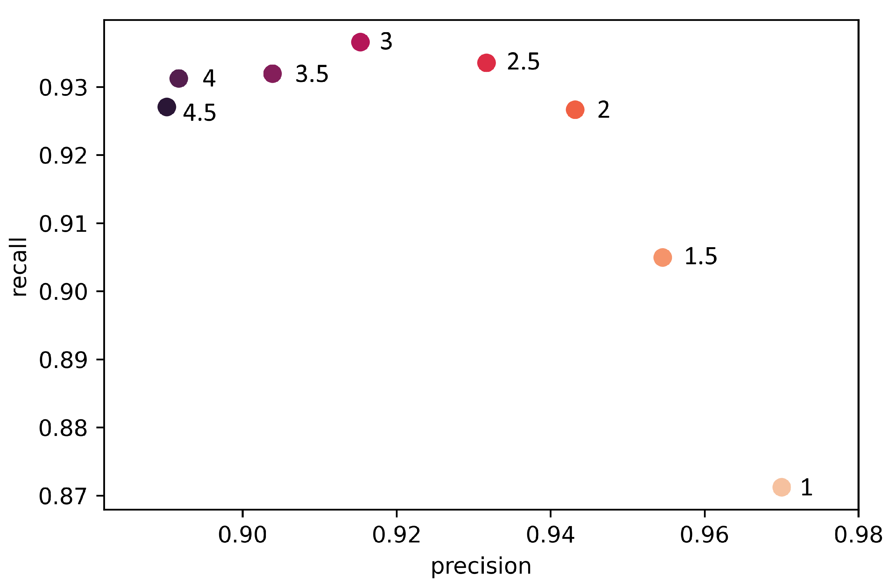
| 3 | 0.9538 | 0.9477 | 0.9620 |
| 2.5 | 0.9544 | 0.9556 | 0.9542 |
| 2 | 0.9534 | 0.9559 | 0.9522 |
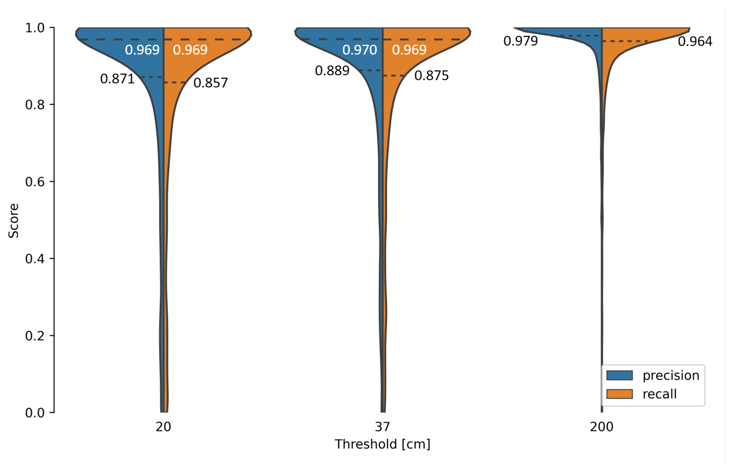
| Threshold (cm) | Mean (cm) | Precision | Recall | |
|---|---|---|---|---|
| 200 | 10.3 | 0.954 | 0.970 | 0.948 |
| 37 | 3.9 | 0.915 | 0.926 | 0.910 |
| 20 | 3.5 | 0.897 | 0.905 | 0.892 |
Publisher’s Note: MDPI stays neutral with regard to jurisdictional claims in published maps and institutional affiliations. |
© 2022 by the authors. Licensee MDPI, Basel, Switzerland. This article is an open access article distributed under the terms and conditions of the Creative Commons Attribution (CC BY) license (https://creativecommons.org/licenses/by/4.0/).
Share and Cite
Lorenzen, S.R.; Riedel, H.; Rupp, M.M.; Schmeiser, L.; Berthold, H.; Firus, A.; Schneider, J. Virtual Axle Detector Based on Analysis of Bridge Acceleration Measurements by Fully Convolutional Network. Sensors 2022, 22, 8963. https://doi.org/10.3390/s22228963
Lorenzen SR, Riedel H, Rupp MM, Schmeiser L, Berthold H, Firus A, Schneider J. Virtual Axle Detector Based on Analysis of Bridge Acceleration Measurements by Fully Convolutional Network. Sensors. 2022; 22(22):8963. https://doi.org/10.3390/s22228963
Chicago/Turabian StyleLorenzen, Steven Robert, Henrik Riedel, Maximilian Michael Rupp, Leon Schmeiser, Hagen Berthold, Andrei Firus, and Jens Schneider. 2022. "Virtual Axle Detector Based on Analysis of Bridge Acceleration Measurements by Fully Convolutional Network" Sensors 22, no. 22: 8963. https://doi.org/10.3390/s22228963