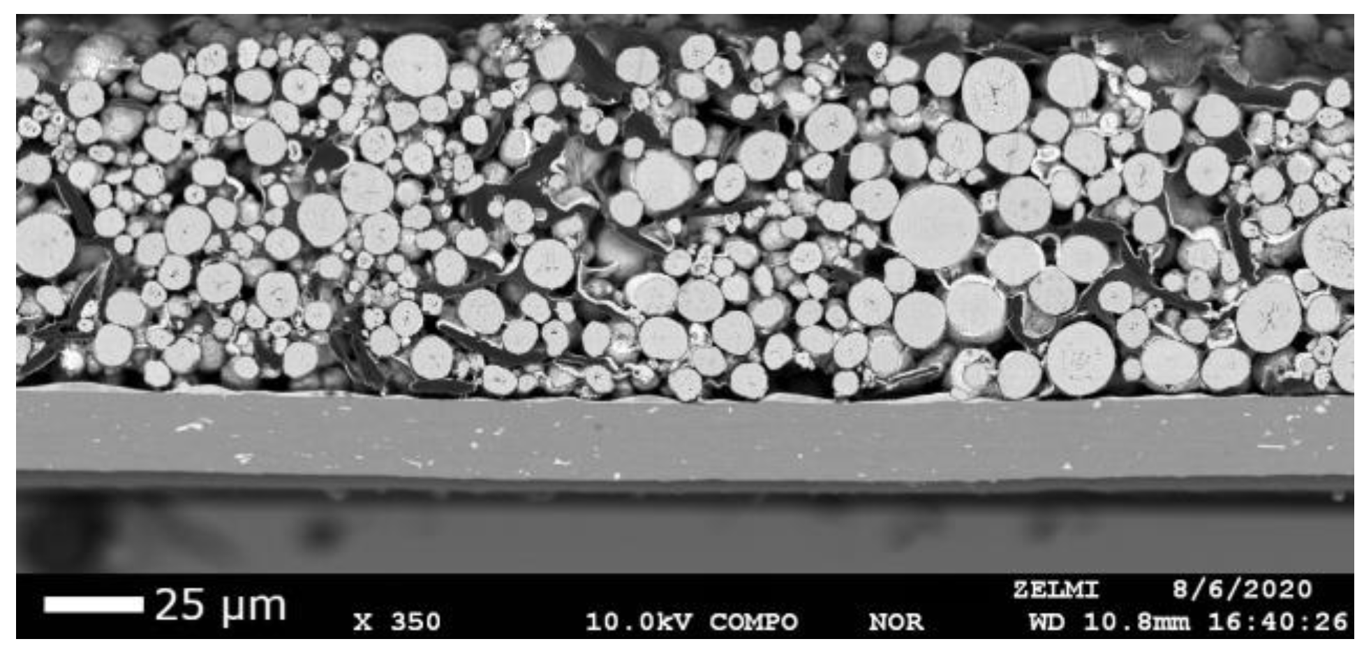
4.1. Cathode Characterization with EMPA
Backscattered electron microscopy has been used to obtain high-resolution images (
Figure 2) of the shape and location of NMC particles.
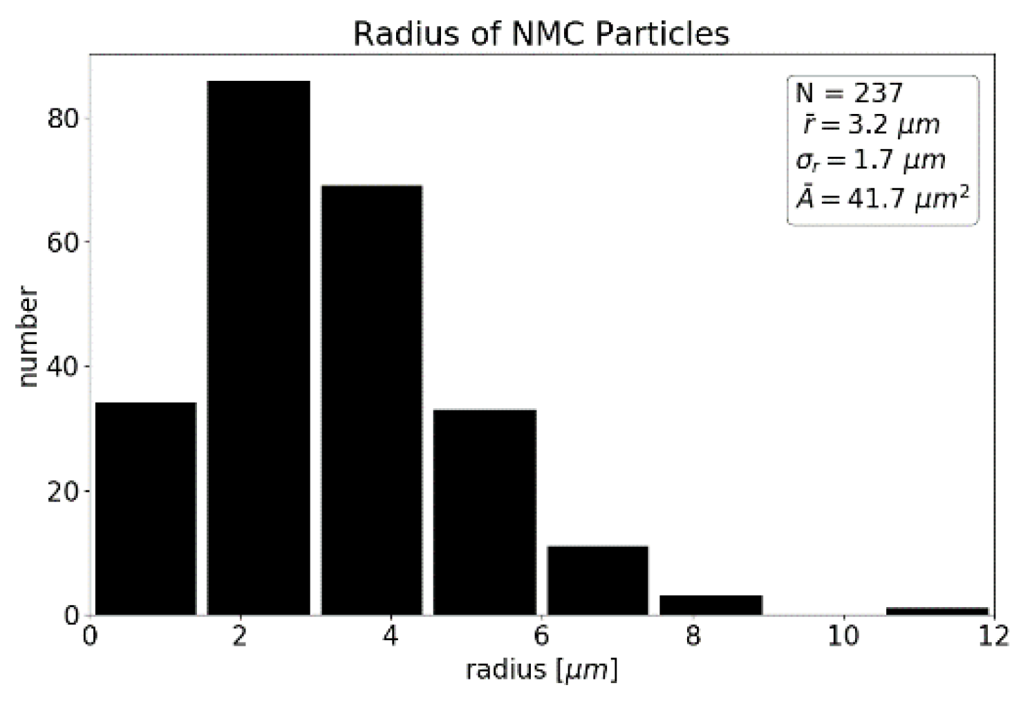
Using OpenCV’s threshold and contour methods, the locations and sizes of the particles were extracted. We determined a mean particle radius of 3.2 ± 1.7 µm (
Figure 3) and a degree of coverage of 38%. This radius may differ from the real particle’s radius since the slice does not cut through every particle in the layout of the maximum cross-section.
The statistical information on NMC particles is essential to interpret spot-to-spot variations in the LIBS measurement. Both limited LIBS-based precision and the granular structure of the sample contribute to spot-to-spot variations in the measured LIBS signal. A detailed quantification of both contributions is necessary to distinguish between expected fluctuations and production-based irregularities. A detailed analysis will be presented in
Section 4.4.
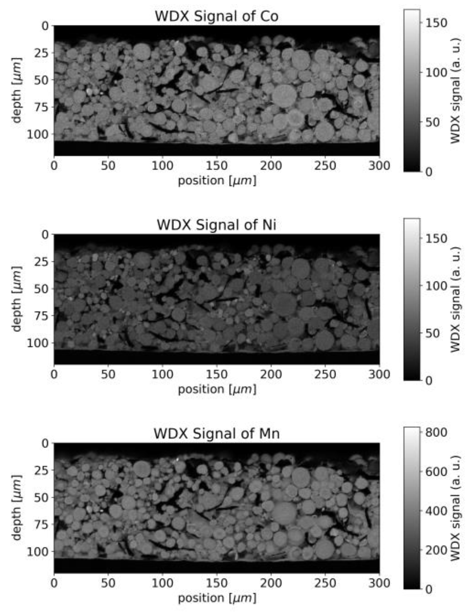
Wavelength-dispersive X-ray spectroscopy (WDX) data supplement the geometrical information with chemical contrast. The WDX signals for Ni, Mn and Co are shown in
Figure 4. Whereas the chemical composition appears homogenous throughout a single particle, slight variations in composition were observed between different particles.
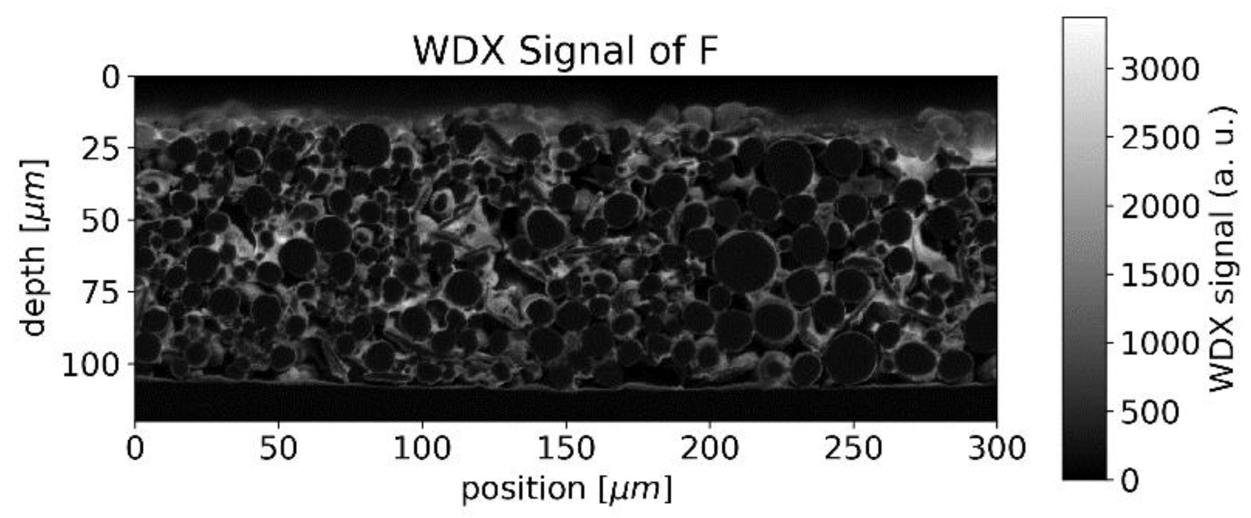
In the case of the binder, which can be identified by the WDX signal of fluorine, accumulations were observed around the surface of the NMC particles, forming rims in the raster image (
Figure 5).
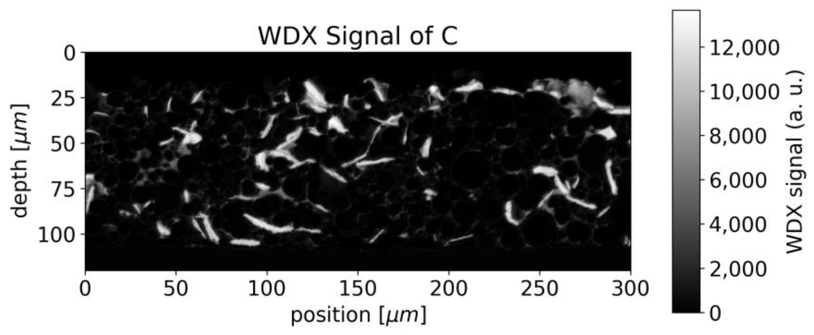
Since both the binder and graphite/carbon black, contain carbon, the distinction between binder and graphite/carbon black is not straightforward. The structure seen in
Figure 5 can also be seen in the WDX signal for carbon (
Figure 6) but superimposed by stronger contributions from the vacancies between different NMC particles, which we assume to be attributed to graphite/carbon black.
The LIBS analysis typically covers a round area of 50 µm waist size and the carbon fluctuations viewed in
Figure 6 would appear smoothed in a single measurement. Averaging is furthermore beneficial due to the limited precision of LIBS in general, but the destruction of the sample at the measurement spot makes repetition impossible at the same position.
4.2. LIBS Measurement
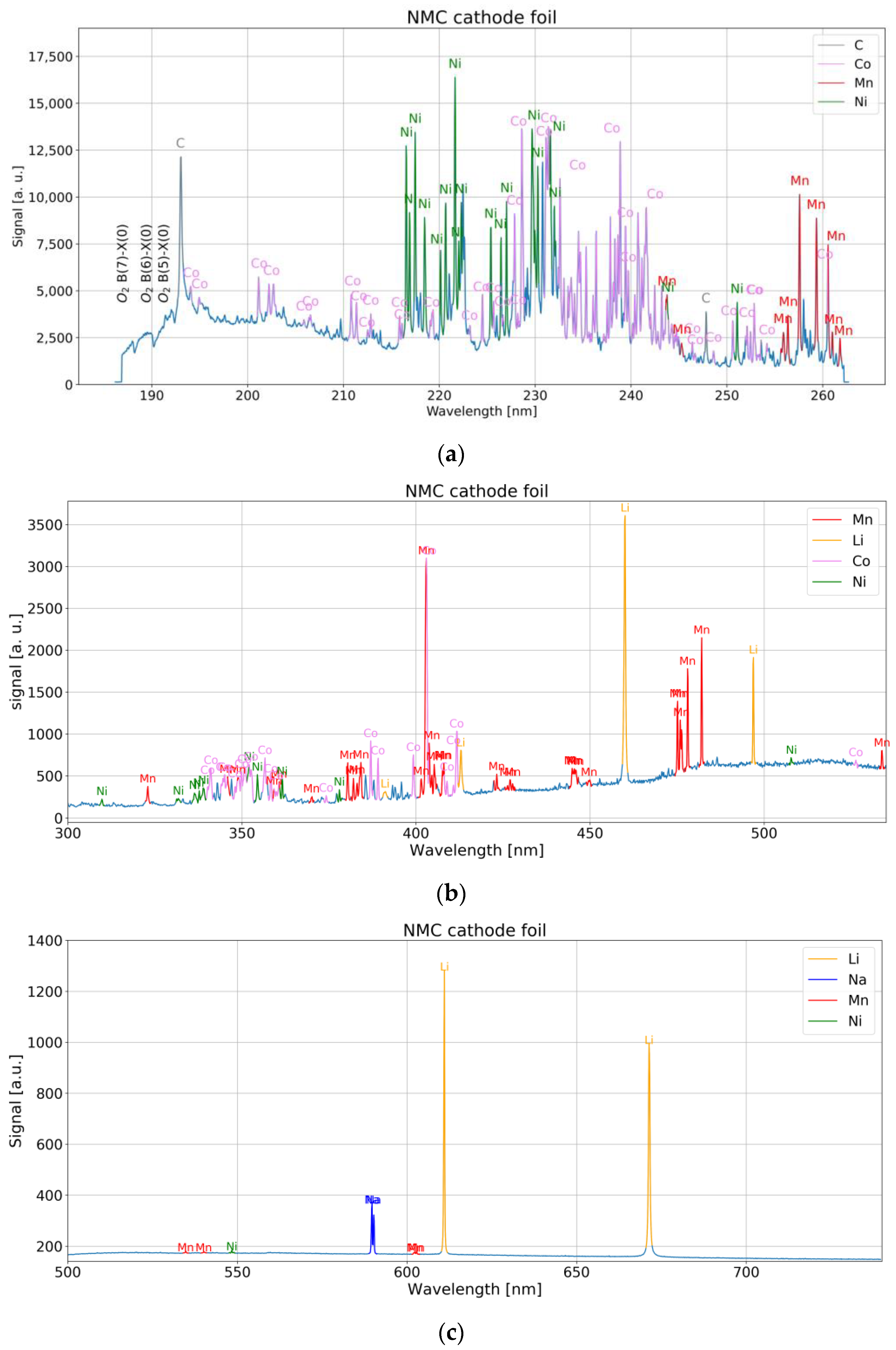
The Czerny–Turner-type spectrometers with mechanically fixed grating cover the whole spectrum of interest for C, Ni, Co, Mn, and Li (193 nm to 671 nm). Corresponding spectra for NMC cathode material are shown in
Figure 7a–c. A small mismatch was observed by comparison of the observed lines with the NIST database [
13]. They are −40 pm (Carbon line) to −100 pm (Manganese line) for the UV device (186 nm–253 nm), −500 pm to –200 pm for the UV-VIS device (270 nm–530 nm) and +400 pm to +700 pm for VIS device (500 nm–730 nm).
Atomic spectral lines of C have been observed from the graphite or binder component. Many strong transitions in the vacuum UV region are present according to spectroscopic databases, but not measurable with a fiber spectrometer and in a LIBS experiment under atmospheric conditions. Nevertheless, single lines in the measurable spectral region at 193.0 nm and 247.9 nm were associated with Carbon.
Molecular bands had been observed in experiments with another laser system in our lab using fs pulses and were mainly attributed to radicals like diatomic carbon, cyano radicals and methylidyne radicals known from the Swan system [
14], initially observed in 1856 [
15]. We noticed that molecular bands and spectral lines were in focus for different adjustments of the detection system, indicating a spatial separation of the different species, as already observed by other groups [
16]. The simultaneous presence of molecular bands and atomic lines made the evaluation of the time-integrated LIBS signal challenging with this laser system.
The major spectral lines of neutral Li are found in the red region of the visible spectrum, namely 670.8 nm (2p → 2s transition) and 610.4 nm (3d → 2p transition) [
13]. The former transition occurs between two states of the same shell which are strongly split due to different Coulomb interactions of the different orbitals to the core electrons and nucleus [
17]. This spectral line suffers from self-absorption [
18] in case of high concentrations which can lead to wrong quantification results, if not accounted for [
19].
The optical emission spectrum of Ni in UV is dominated by transitions of the outmost electrons, namely the eight d electrons and the two outer s electrons. The strongest lines either involve the ground level configuration 3d
8(3F)4s
2 or the 3d
9(2D)4s configuration. A high density of states is found in the range 3.3 eV–4.2 eV (spectral lines between 280 nm and 400 nm), around 5.3 eV–5.6 eV (spectral lines in the range 228 nm–242 nm) and for energies larger than 6 eV [
13].
Similar to Ni, the Co emission in the visible spectrum is governed by transitions of the seven d electrons and the outmost two s electrons. Several different terms for the configurations 3p63d74s2, 3p63d84s and 3p63d84s4p are responsible for a great number of transitions mainly in the UV spectrum shorter than 300 nm.
For Mn, excited states are lifted at least 2.1 eV from the ground level. A high density of states is found in the range 2.1–2.3 eV, 2.9–3.4 eV and 3.7–3.9 eV. For energies > 4.2 eV many states are registered. Most of the prominent lines involve either the ground level (distinct lines at 279 nm, 322 nm, 403 nm, 539 nm) or a lower level in the range 2.1–2.3 eV (lines in the ranges 304–307 nm, 320–327 nm, 353 nm–373 nm, 379 nm–385 nm and 404 nm–408 nm) [
13].
For Al, NIST data [
13] show a large separation of 3.1 eV between the ground state and the excited states. Above 4.8 eV, the density of states is highly increased. Several terms at 3.1 eV, 3.6 eV, 4.1 eV and 4.6 eV are responsible for strong lines around 395 nm, 309 nm, 257 nm and 265–266 nm in the UV spectrum. Although detected in the spectrum, ionic Al II lines turned out to be much more intense compared to Al I lines and were subsequently used. The most prominent line of Al II detected in our measurement was between 198 nm and 199 nm.
It is worth mentioning that spectral features were observed around 185 nm–193 nm, which we ascribe to Schumann-Runge bands of O
2 [
20].
4.3. Concentration Measurement
For quantitative analysis, the LIBS system was calibrated on NMC 111 samples with different mass concentrations of graphite/carbon black (0–15%) and binder (6–11%). We observed an increase in the intensity of carbon lines with respect to metallic lines for increasing pulse energy in the range below 2 mJ, which potentially indicates non-stoichiometric ablation [
21]. Calibration measurements were performed at 6 mJ, in the stable region above 3.5 mJ.
The large fluctuation in the intensity of spectral lines between successive laser pulses makes quantitative analysis directly from the line intensity challenging. This problem is often met with normalization methods, e.g., internal standard [
22], standard normal variate of the whole spectrum, area under the spectrum, or background. Several publications treat the problem of selecting appropriate lines such as avoiding or dealing with resonant [
23] and self-absorbing lines of major components. The selection of lines with similar upper energy levels can minimize the influence of changing plasma parameters [
24]. For C, both observed lines in the UV spectrum, 193 nm and 248 nm share the same upper energy level (2s
23p3s (1P)) of 7.68 eV. This is comparable with the first ionization energy of Co (7.88 eV), Ni (7.61 eV) and Mn (7.43 eV), and therefore, larger than the typical upper energy levels of intensive lines in the spectrum from NMC targets [
13]. Taking the intensity ratio of two spectral lines with different upper energy levels makes the measurement plasma temperature dependent. Nevertheless, reproducible calibration curves were achieved with normalization to the standard normal variate of the spectrum which we did for all evaluations shown in the following.
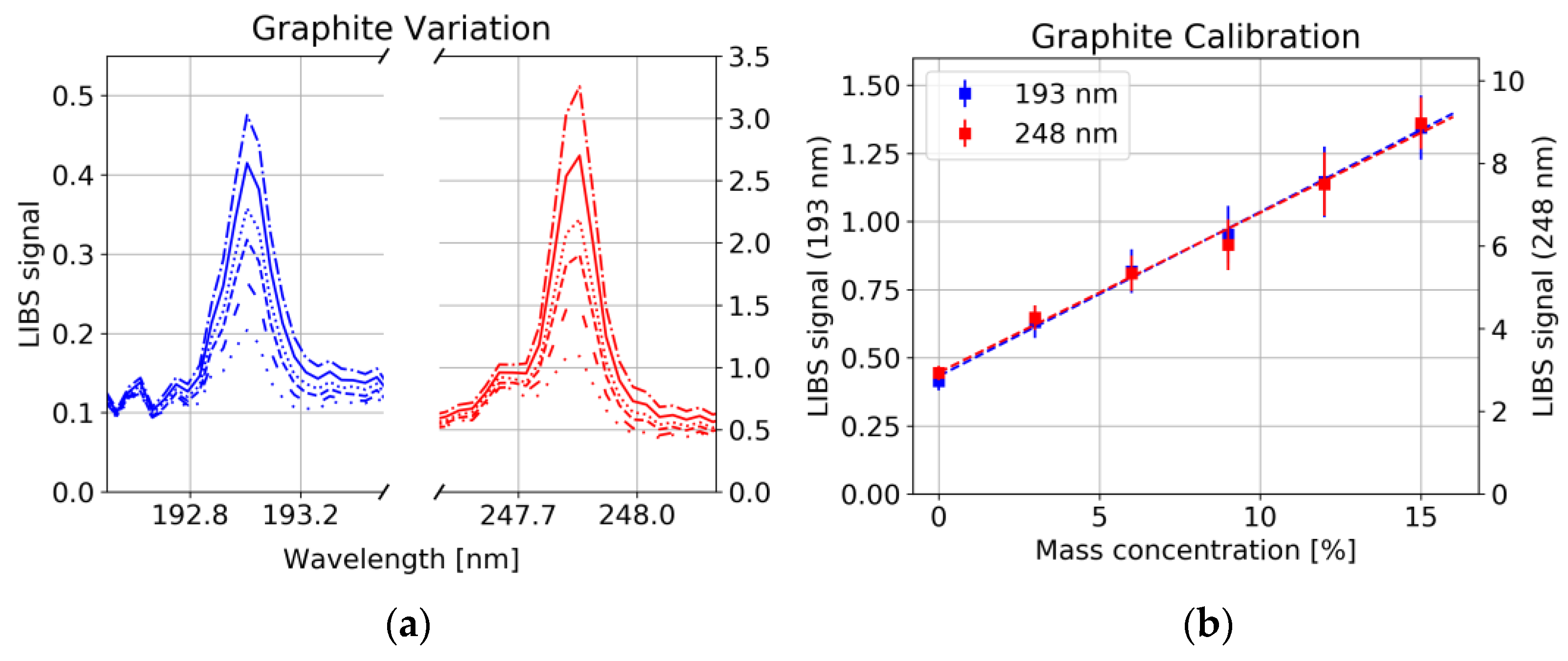
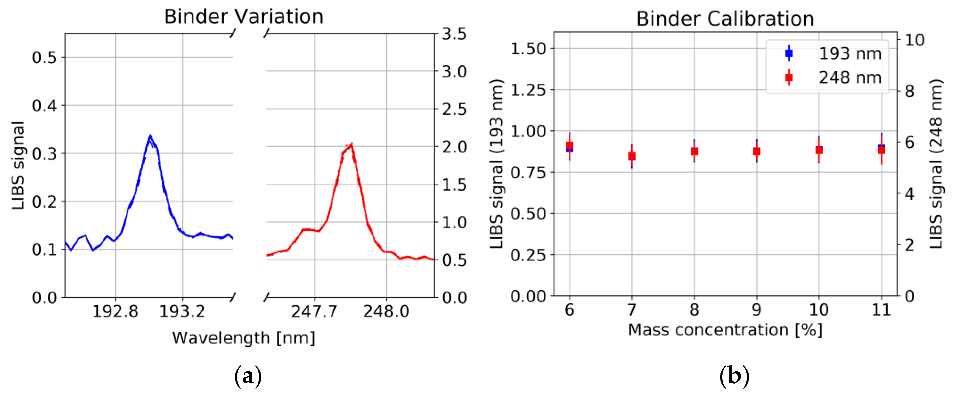
A strong correlation between the 193 nm as well as the 248 nm carbon line with the graphite/carbon black concentration was observed (
Figure 8a, Pearson correlation coefficient R
2 = 0.997), whereas the concentration of binder had no significant influence on the line intensity of C (
Figure 9a). This could have several reasons: 1. Non-stoichiometric ablation of the sample, i.e., only little amount of the binder enters the plasma, whereas graphite/carbon black is easily ablated. 2. Long-chained polymer binder rather forms molecules instead of atomic species [
25]. 3. Different plasma conditions, e.g., lower plasma temperature in the polymer containing plasma, prevent the upper energy level corresponding to the 193 nm and 248 nm line to be occupied.
For each of the six samples, 25 measurements were taken at each of the 25 measurement spots. The average was taken over all measurements at the same spot. From those 25 spectra, the C signal was evaluated from the spectral region between 192.8 nm and 193.3 nm (247.7 and 248.0 nm) by dividing the baseline-corrected area through the standard normal variate of the whole spectrum.
Figure 8b shows calibration curves together with the point-to-point deviation of the LIBS signal illustrated by error bars. Besides the growing standard deviation with increasing graphite/carbon black content, a significant Y offset has been observed which can hardly be explained by interference with other spectral lines. On the other hand, as already mentioned above and shown in
Figure 9b, a variation of binder shows no significant influence on either the carbon signal. This offset could be due to residues from the solvent remaining in the sample. Further investigations are needed to identify the cause.
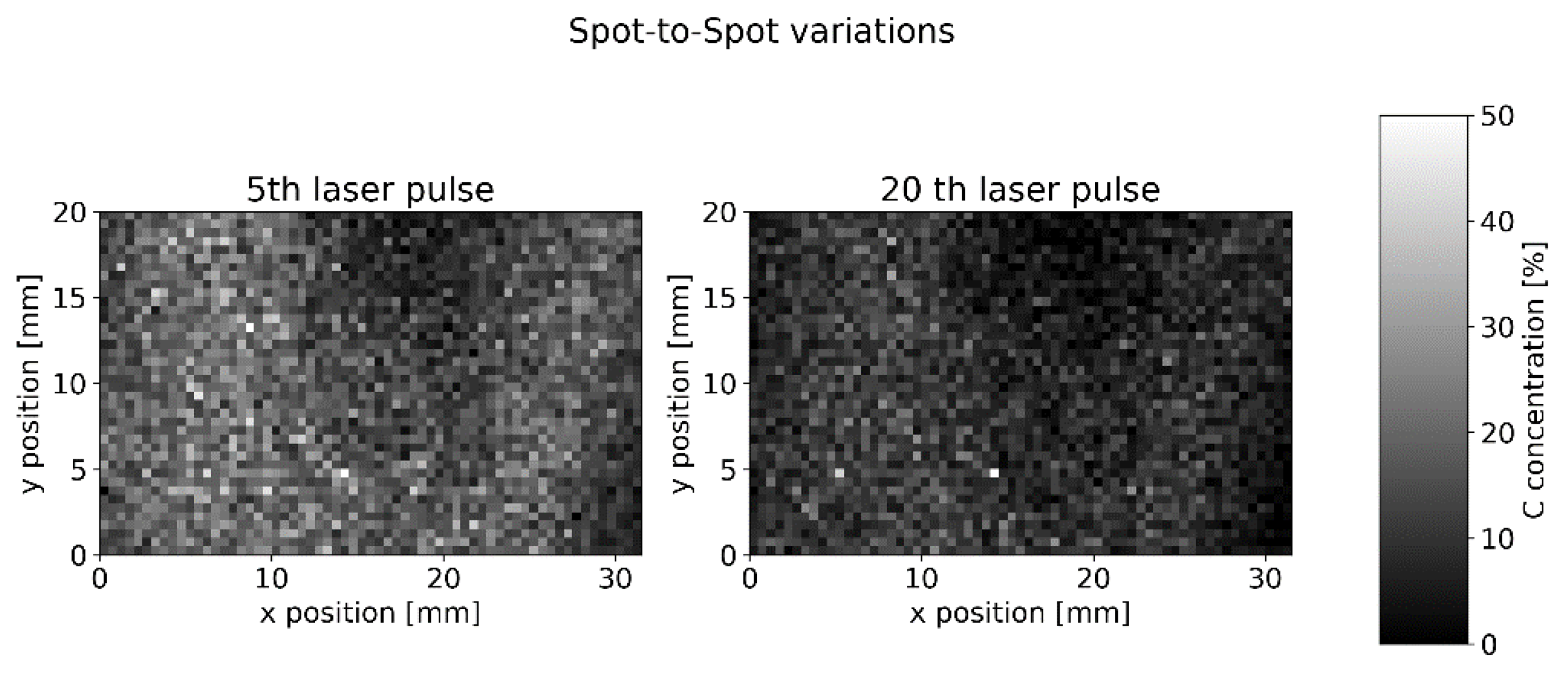
Detailed statistics on spot-to-spot signal variations were gained from a 31.5 mm × 20 mm measurement field with 2520 measurement spots and 60 laser pulses at each position (
Figure 10).
The mean spot-to-spot standard derivation inside each layer is 27.3%. We will show in the next section that we expect a similar value due to the inhomogeneity of our cathode sample.
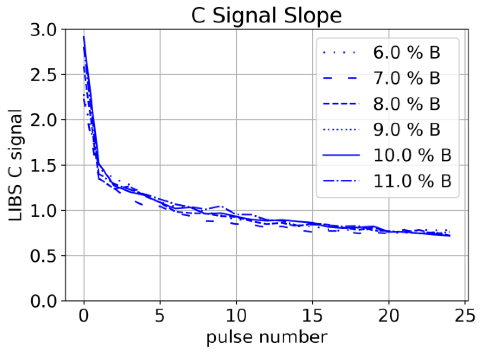
A decrease in Carbon signal has been observed systematically for subsequent laser pulses at the same spot (
Figure 11). Since this decrease is again independent of the binder concentration, we conclude that it is related to the ablation of graphite/carbon black. We interpret this observation as a result of a lower ablation threshold of graphite/carbon black compared to other constituents and conclude that uniform depth profiling is challenging with this composition of the material.
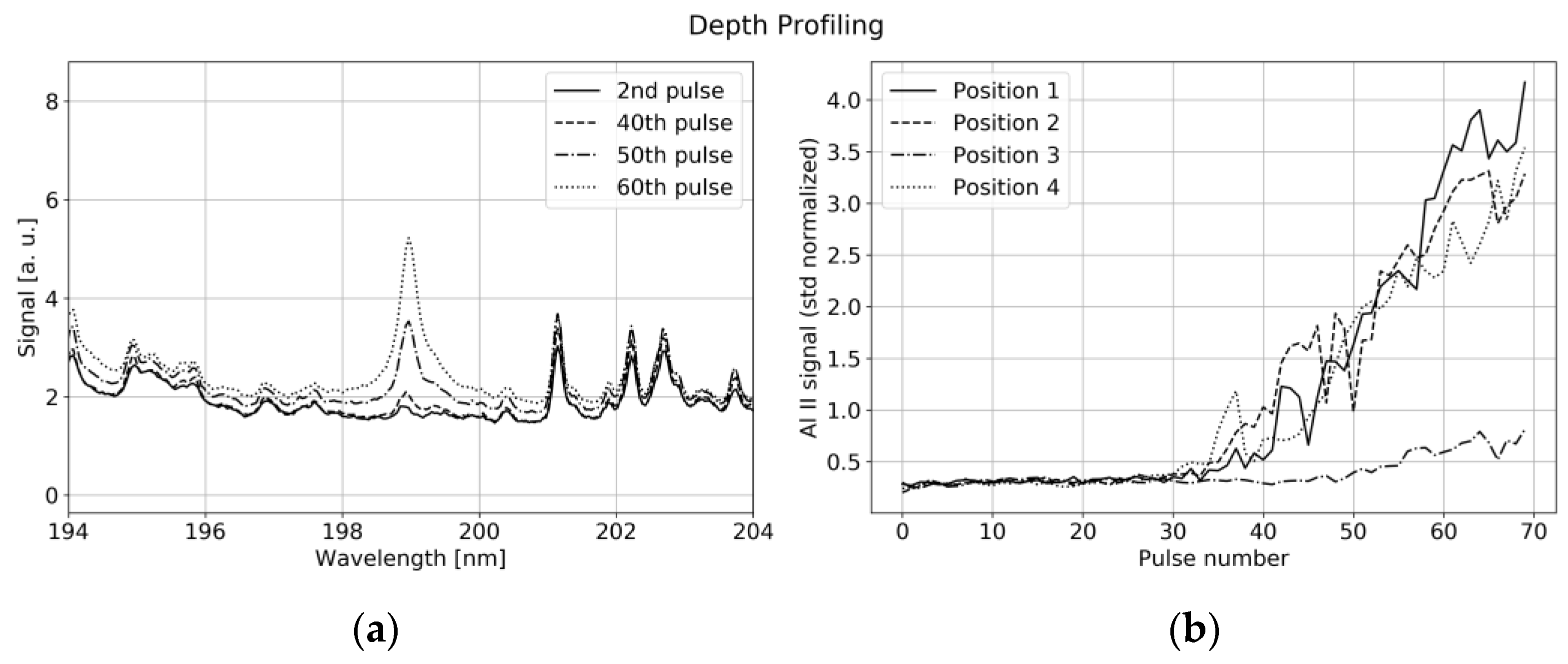
Nevertheless, reproducible depth profiling is possible with some limitations: As illustrated in
Figure 12a, the aluminum current collector is uncovered with subsequent laser pulses leading to a strong increase in the single-ionized aluminum (Al II) line at 198.8 nm. The ablation rate significantly changes with laser power. The Al II signal is viewed in
Figure 12b for subsequent laser pulses with 6 mJ energy per pulse at four different positions.
Although the evolution of the Al II line showed good agreement for many different measurement points, a comparison with microscopic images pointed out, that the ablation rate significantly depends on the particle distribution at the specific position. The presence of large NMC particles slows down the uncovering process, as shown in
Figure 12b (position 4), while the ablation rate of binder and graphite turns out to be higher. This leads to protruding NMC particles around the already vaporized binder and graphite/carbon black areas at the measurement spot. Additionally, the Gaussian profile of our laser beam together with the thermal conductivity of the sample leads to a V-shaped crater, which makes a difference between the profiles shown in
Figure 12b and a step function. We conclude, that under ideal conditions, i.e., controlled distance to sample and constant laser power, our system is able to detect relative depth variations in the order of 20% for depths in the range of 25–100 µm.
4.4. Cathode Characterization with EMPA
Given that a single LIBS pulse takes the average concentration inside the focal area of the excitation beam, the measurement can be understood as a smoothing operation of the local concentration within the beam’s waist size w. We consider the smoothing kernel:
Its spatial Fourier transform corresponds to the transfer function and is given by:
The transfer function quantifies how spatial frequencies of concentrations are “smoothed out” by averaging over the measurement spot. When fluctuations are taking place on small length scales compared to the laser spot size, the measured variations are smoothed out efficiently by the extent of the laser spot. It is, therefore, instructive to quantify the spatial frequencies of local concentrations by Fourier transform and compare it to the transfer function H.
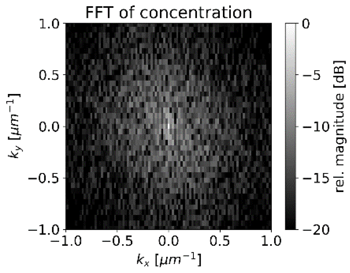
For the spatial carbon distribution of
Figure 6, we obtain the discrete Fourier transform as illustrated in
Figure 13 with a logarithmic scale.
The center of
Figure 13 represents the average concentration of the whole measurement area whereas the points around correspond to amplitudes of concentration variations with different spatial frequencies. The pixels in
Figure 13 are not square due to different pixel numbers in the x and y directions in
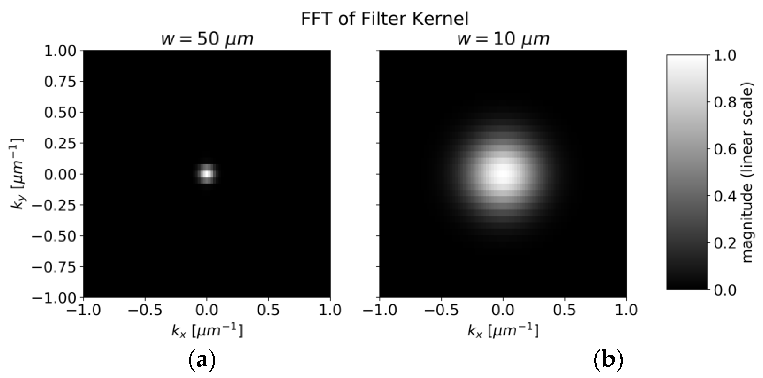
Figure 6. The smoothing operation suppresses higher frequencies by multiplying the data pointwise with
H (shown in
Figure 14). The radius of the transfer function’s spot is inversely proportional to the laser spot’s radius. After smoothing, the squared sum of remaining amplitudes for frequencies other than (0 µm
−1,0 µm
−1) represents the expected amplitude of fluctuations.
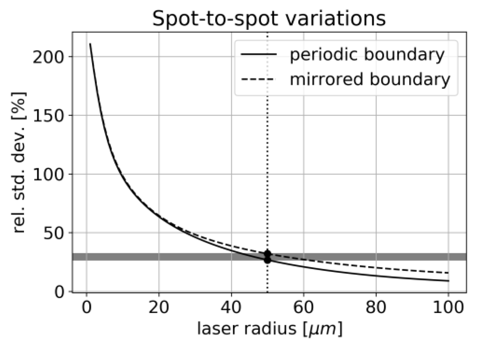
For the chosen dataset, the relative amplitude of fluctuations is compared for different laser spot sizes in
Figure 15.
We, therefore, expect a strong dependency between laser spot size and signal variance for this kind of inhomogeneous sample. For a laser waist size of 50 µm, we obtain an expected relative variance of 27–32% which is in good agreement with the data shown in
Figure 6 Thus, the laser spot radius appears as an important parameter when measuring inhomogeneous samples and needs to be compared to the typical length-scale of the structure.

 and
and 


