
A Probabilistic Approach to Estimating Allowed SNR Values for Automotive LiDARs in “Smart Cities” under Various External Influences

 ,
,  , , ,
, , ,
Abstract
:1. Introduction
2. Theoretical Aspects of the Study of Diffuse Interference
2.1. Physical Basis of Laser Radiation
2.2. Methods of Forming a Multibeam Structure
2.2.1. Lidars with a Line of Lasers
2.2.2. Lidars Using Matrix Lasers
2.2.3. Lidars with Diffractive Optical Elements
2.3. Calculating the Distance from the LiDAR to the Object
2.3.1. Time-of-Flight Methodology
- c—speed of light;
- τp—probe pulse duration;
- n—is the refractive index of the transmission medium (taken as 1 for air).
2.3.2. Phase Comparison Methodology
- temperature increase/decrease;
- high humidity;
- dust particles in the atmosphere;
- scattered radiation from other laser sources located within reach;
- direct radiation from other laser radiation sources located within reach.
3. Intentional Impacts on the LiDARs
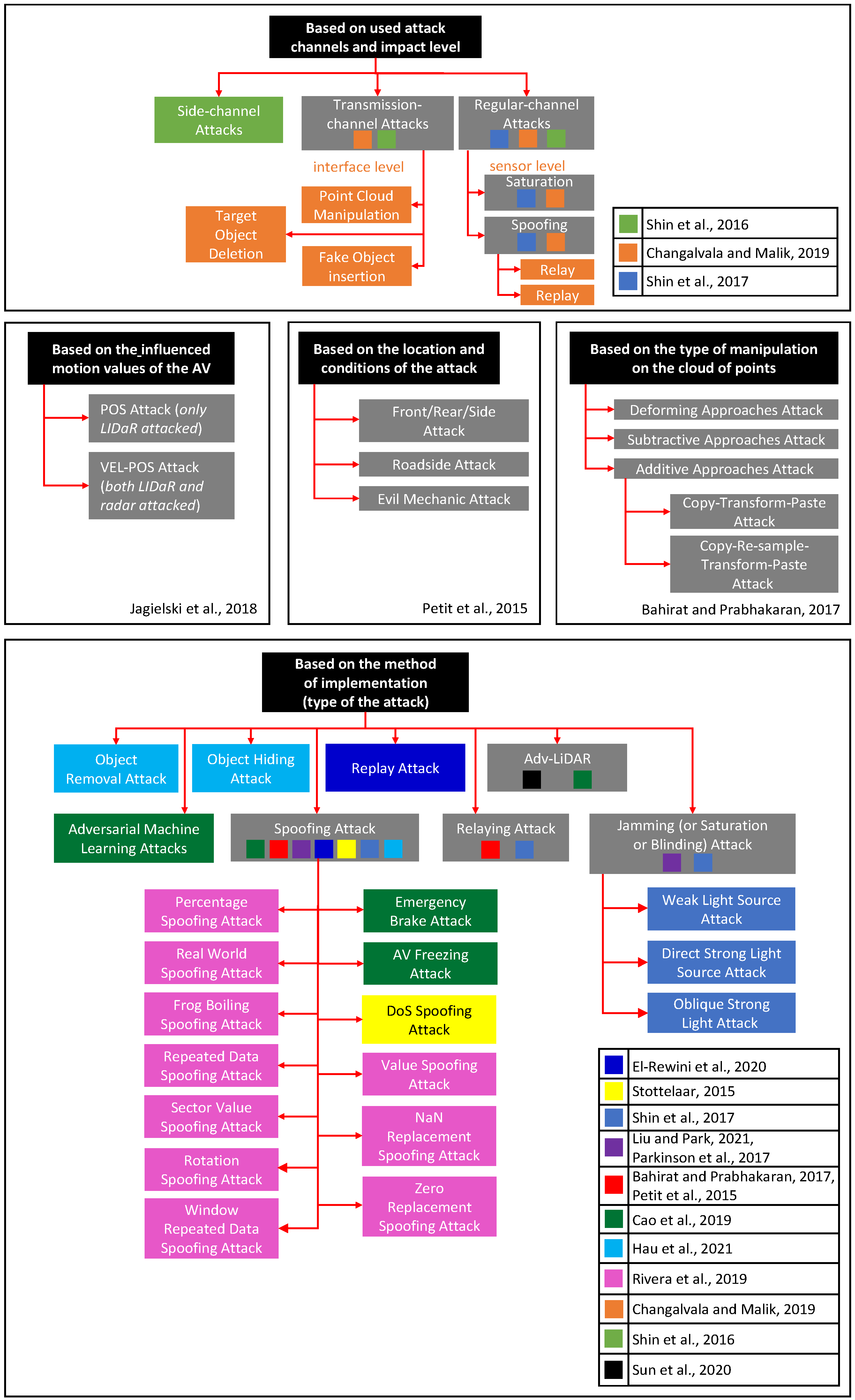
3.1. Classification of Attacks on AV LiDARs
- Cao et al. [14] distinguish LiDAR spoofing attacks (injecting fake points in the LiDAR’s cloud using lasers; emergency brake attack, and AV freezing attack as particular implementations) and adversarial machine learning attacks (crafting and putting object on the scene to deceive the LiDAR’s detection system);
- In addition to classifying attacks by type of points manipulation, Bahirat and Prabhakara [13] specify relaying and spoofing attacks;
- Stottelaar [15] describes jamming, relaying, spoofing, and denial-of-service (DoS) attacks;
- Shin et al. [10] classify sensor spoofing, spoofing by relaying, and sensor saturating attacks. Sensor saturating attack is also called blinding attack and has specific scenarios that can also be considered as its implementations: weak light source, direct strong light source, and oblique strong light source saturating attacks;
- Hau et al. [16] refer to LiDAR spoofing, object hiding, as well as object removal attacks;
- Petit et al. [11], considering attacks on LiDARs separately, describe relaying and spoofing attacks;
- El-Rewini et al. [19] distinguish replay, relay, blinding, spoofing, jamming, and DoS spoofing attacks;
- Among the implementations of spoofing attacks, Rivera et al. [20] singled out several in terms of the impact on the LiDAR’s state: percentage spoofing attack, value spoofing attack, rotation spoofing attack, zero replacement spoofing attack, NaN replacement spoofing attack, repeated data spoofing attack, window repeated data spoofing attack, sector value spoofing attack, real world spoofing attack, and Frog Boiling spoofing attack. They can also be considered as specific implementations of a spoofing attack (highlighting the influence of the LiDAR’s state as a separate basis for the classification is not advisable due to considering different variants of only one type of attack).
3.2. An Overview of Current Attack Vectors on the Automotive LiDARs
3.2.1. Adversarial Attack
3.2.2. Spoofing Attacks
- POS attack: Implementing LiDAR spoofing to deceive the AV’s position in space.
- VEL-POS attack: A POS attack simultaneously spoofing AV’s speed values (radar attack).
- Signal replay attack. The attacker constantly receives and records LiDAR signals and then sends them back, resulting in forming a cloud of points for a nonexistent object [15,19,29]. Another example of such an attack is the study [30] where the authors used Raspberry Pi and a low-power laser to compromise the LiDAR, as well as to create a fake obstacle for the AV, which led to its emergency braking.
- Signal relay attack (or “spoofing by relaying” as stated in [10]). The LiDAR signal is received by the attacker (photodiode is usually used for synchronization purpose), recorded and transmitted to a transceiver located elsewhere from where the signal is transmitted back to LiDAR (with a certain and configurable delay) using an “attack” laser triggered by a specially crafted pulse waveform. This creates fake echoes. By changing the delay value, the attacker can “select” fake points to be inserted into the point cloud. Such an attack can lead to distortion in mapping of the objects (real objects will be further or closer to their respective cloud of points formed by the LiDAR). For example, in the work [11], the cheap Osram SFH-213 photodetector and Osram SPL-PL90 laser were used to conduct such an attack (target LiDAR—ibeo LUX 3). As a result of injection of counterfeit points into the point cloud, the LiDAR detected a non-existing wall.
- In [10], a signal relay spoofing attack, experimentally verified using the Velodyne’s VLP-16 LiDAR, has been described and carried out. The photodiode and pulsed laser diode used are similar to [11]. The attack to spoof the LiDAR created an obstacle that was closer to the AV than the location of the attacker (the device used to a spoof the LiDAR).
- Adv-LiDAR. Due to the wide range of considered issues, and the use of a new type of LiDAR vulnerability (ignoring occlusion information in the point clouds by the LiDAR’s perception models), results obtained by Cao et al. [14] should be regarded as a separate spoofing attack implementation. The authors managed to create about 100 fake points at once at a distance of more than 10 m, and algorithm presented in the work allowed to increase the success rates on average 2.65 times (in Baidu Apollo LIDAR perception module, overall attack success rate of 75%). It is assumed that the attacker can act both independently (as a pedestrian influencing the AV) and while inside the other AV moving in the adjacent traffic lane. As a result of the attack, the target AV had to stop abruptly (from 43 km/h to 0 km/h in 1 s), which in real-world conditions could lead to serious consequences. The proposed Adv-LiDAR approach in addition to spoofing attack also used adversarial machine learning methods to deceive the very algorithm of LiDAR’s perception (experiments based on the Baidu Apollo 3.0 model and their Sim-control AV simulator, known photodiode and a laser diode [10,11] were used to physically attack the LiDAR, the “victim” was Velodyne’s VLP-16 PUCK LiDAR). Thus, Adv-LiDAR includes both spoofing attack and adversarial machine learning attack techniques, and thus belongs to both types of the attacks on automotive LiDARs.
- Emergency brake attack. Adversarial 3D point cloud creates spoofed obstacle that is in “located” in front of the AV, in close proximity to it. This forces the AV’s self-driving system to use emergency brake system to avoid a fake obstacle;
- AV freezing attack. A front-side obstacle is spoofed by creating an adversarial 3D point cloud in front of the AV (and in close proximity to it). In the case of being in a stationary position at the time of the attack, the AV will not be unable to start moving.
- 5.
- DoS spoofing attack. In papers [15,19], the DoS attack stands out as one of the most appropriate implementations for this type of attack. It is assumed that the attacker’s objective is to spoof the LiDAR via the injection as many fake points as possible. This will result in ample false 3D objects to exceed the maximum number of trackable objects of the target LiDAR.
- 6.
- As mentioned earlier, the authors of [20] divide the spoofing attack based on the effect on the current state of the LiDAR, since the attack vectors are irrelevant. In particular, the article singles out the following attacks (given with a short description corresponding to the content of the work [20]):
- percentage spoofing attack: increasing input values by a specified percentage;
- value spoofing attack: shifting points in the cloud via a given value;
- rotation spoofing attack: changing only the indices of the measured values array;
- zero replacement spoofing attack and NaN replacement spoofing attack;
- repeated data spoofing attack: looping the replay of the input;
- window repeated data spoofing attack: looping the repeat of some value (or a number of values) as an input in a form of a sliding window;
- sector value spoofing attack: relay of a fake LiDAR signal from a certain direction;
- real world spoofing attack: only part of the LiDAR point cloud is affected, which corresponds to actual external attacks using additional equipment (e.g., laser);
- Frog Boiling spoofing attack: scrupulous change of the LiDAR’s input (one or several points in the cloud) below the detection filter (threshold value) to avoid attack detection (attack named in accordance with [31]).
3.2.3. Saturation Attack
3.2.4. Other Attacks on the LiDAR
- Cloud points manipulations using raw data. The authors [13] distinguish three groups of forgery attacks on the LiDAR, based on the method of changes: additive approaches attacks, subtractive approaches attack, and deforming approaches attack. The additive approaches attacks imply adding new points to create an object on the scene, subtractive approaches attack—removing the points that make up an object to delete it from the scene, while in the deforming approaches attack the surface and/or the shape of the object are deformed by altering the position of a number of points. The points’ position shift may lead to incorrect detection of the object or even its non-detection by the LiDAR. Two implementations of additive approaches attacks are given: a copy-transform-paste attack and a copy-re-sample-transform-paste attack. The latter one allows matching the forged object to the LiDAR’s resolution to be placed in the dot cloud (on the stage) properly. The proposed attacks are similar to both adversarial and spoofing ones. Despite this, these attacks cannot be defined as spoofing attacks, as the paper explicitly states that no additional hardware is required for these attacks, i.e., the creation/removal/changing of the points in the cloud cannot be performed via sending fake signal to the LiDAR. In addition, there is also no indication that the described attacks are intended to be used to mislead recognition and machine learning systems, which also prevents them from being classified as adversarial machine learning attacks. Thus, the described attacks are introduced into a separate class. As stated in Section 2.1, this type of attack belongs to transmission-channel ones.
- Using objects with surfaces of extremely high reflectivity or absorptive capacity. Petit et.al. suggested to use special surfaces with increased reflection or absorption values for infrared light, which can lead to the formation of a fake cloud of points, hinder the detection of objects with distorted shapes and dimensions or total/partial malfunction of LiDAR’s detection system [32]. Still on this topic, over the last few years, materials and paints with extremely high reflectivity values have been created, e.g., (but not limited to) Vantablack and Vantablack 2.0 [33], Black 3.0 [34], Musou Black, “dark chamaleon dimers”, etc. For example, the latter, being a nanostructured material, can absorb up to 98–99% of light rays in 400–1400 nm wavelength range, with no relevance to the angle and polarization type of falling light [35], and the BMW managed to introduce their X6 car coated with Vantablack [36]. Considering that LiDARs mostly function at 905, 940, and 1550 nm wavelengths [37], the studies of LiDAR behavior in the presence of objects (or cars) with the above materials and paints (or coatings with high reflectivity values) should be relevant. Whether such objects pose a threat to LiDARs and/or AV’s ADAS remains an open question (at least in this paper).
- Side-channel attacks. Such attacks are based on receiving (extracting/intercepting) the useful signal due to the physical implementation of target systems, the generated physical fields, or the physics of the processes occurring therein. Possible LiDAR attacks can be based on timing, power consumption, and electromagnetic emissions. For example, it can be assumed that since the LiDAR converts the value of laser pulse intensity into electrical signals [17] and contains electronic components, it should be susceptible to leaks of useful signals through various types of parasitic emissions of its electronic equipment (TEMPEST), while small fluctuations of the voltage consumed may be correlated with the features of microcontrollers and electronic control units (ECUs). In the first case, the attacker can intercept the compromising electromagnetic radiation and extract the useful component of the signal. In the second case, they can figure out the logic and the time parameters of the computational operations performed. We failed to find any open-source studies concerning the implementation of side-channel attacks on the automotive LiDARs. Despite this, the study of LiDAR side-channel attacks seems to be relevant.
- Lidar’s ECU malware attack. Infection of the ECU via the malware can cause both DoS of the LiDAR (or the whole AV at once) and malicious disturbances in its functioning [22]. Such an attack can be carried out if the intruder has physical access to the AV (e.g., Evil Mechanic attack [11]) or through the adversary impact on the ECU (for example, when upgrading firmware; over-the-air attack) [38]. Such attacks can seriously compromise the safety of the autonomous vehicles, transported passengers or cargo, and other road users.
- Evil sensor calibrator and data fusion manipulator attacks. Navigational data fusion algorithms are designed to provide redundant information on AV motion parameters, its position, and the characteristics of other traffic participants, as well as the infrastructure of a “smart city” (in both local and global coordinate systems). In turn, sensor calibration and pairing procedures are designed to compare data from different sensors and systems for further processing, including to ensure mutual correction and correct operation of the AV in cases when one or more sensors have failed. An attacker may interfere with the calibration process of a pair of sensors (evil sensor calibrator attack), one of which is LiDAR (e.g., LiDAR-GNSS, LiDAR-IMU, LiDAR-camera, etc.), or the algorithms of data fusion in the navigation subsystem (call it fusion data manipulation attack). As a result, the algorithms and methods used in the LiDAR or its ECU to counteract spoofing or other adverse effects (if any) will not be effective, as correcting the LiDAR readings from other sensors and systems will not be possible. The resilience of the AV’s navigation system will be impaired, and ECU will receive false information about traffic parameters and the location of the AV on the road, which could lead to accidents [38].
4. Unintentional Adverse Impact on the LiDARs
4.1. Classification of Unintentional Impacts on LiDARs and Their Sources
4.2. LiDAR Mutual Interference Theories
4.3. The Influence of Harsh Weather and the Environment on the LiDARs
5. Improving LiDAR’s Security and Resilience by Mitigating Negative External Impacts
5.1. Increasing the Resilience to Mutual LiDAR Interference
- frequency-hopping modulated LiDAR for autonomous vehicles [64];
- FPGA-based dual-pulse LiDAR with digital chaotic pulse position modulation [65];
- CMOS LiDAR sensor with a SPAD-based random number generator and high background noise immunity to detect time-correlated TOF [66];
- chaotic laser imaging lidar based on the orthogonality of the Boolean chaotic waveform;
- SPAD-based LiDAR with photon-driven stochastic pulse position modulation [67];
- software-based optical sampling scheme for ToF LiDAR with pseudo-random binary sequences [68];
- interference-robust CDMA LiDAR [69];
- interference-resistant 3D Pulsed Chaos lidar [70].
5.2. Methods of Protection against LiDAR Attacks
- the use of density consistency check approach to detect false points in the cloud (Bahirat and Prabhakaran [13]);
- the use of 3D temporal consistency check to verify detected objects (You et al. [73]);
- watermark insertion into the data of the LiDAR to detect and localize fake object insertion and deletion (Changalvala and Malik [9]);
- utilizing vehicle-to-vehicle links to increase situational awareness using measurements of other AVs (Stottelaar [15]);
- LIFE (LIDAR and Image data Fusion for detecting perception Errors)—LiDAR and camera data comparison method based on spatial and temporal features to detect data anomaly (Liu and Park [17]);
- occlusion-aware hierarchy anomaly detection (CARLO)—an occlusion-based approach to detect laser spoofing attacks (Sun et al. [21]).
5.3. LiDAR Resilience Improvement via Increasing the SNR
6. Proposed Method
6.1. Approach to Estimating the Probability of Detecting a Reflected Pulse in Space
- This approach has been tested using ideal environmental parameters (normal LIDAR operating conditions) and did not take into account the background changes of the environment. Further studies are expected to take into account background noise caused by sunlight in clear weather conditions.
- The quality of the point cloud is not taken into account. Instead, the probability value of false alarm is stabilized in relation to the maximum probability of correct response. Since the probability of a false event occurrence is not known at every moment of time, it is possible to apply the Neyman–Pearson criterion when choosing the solution.
- The approach does not allow to quantify the elements of various types of errors from the sources of uncertainty.
- The study did not identify clearly defined sources of uncertainty in different LiDAR subsystems, only the resulting error has been estimated.
- Errors caused by the environmental noise have not been into account separately, but their overall contribution to the background error has been considered.
6.2. Description of the Proposed Approach
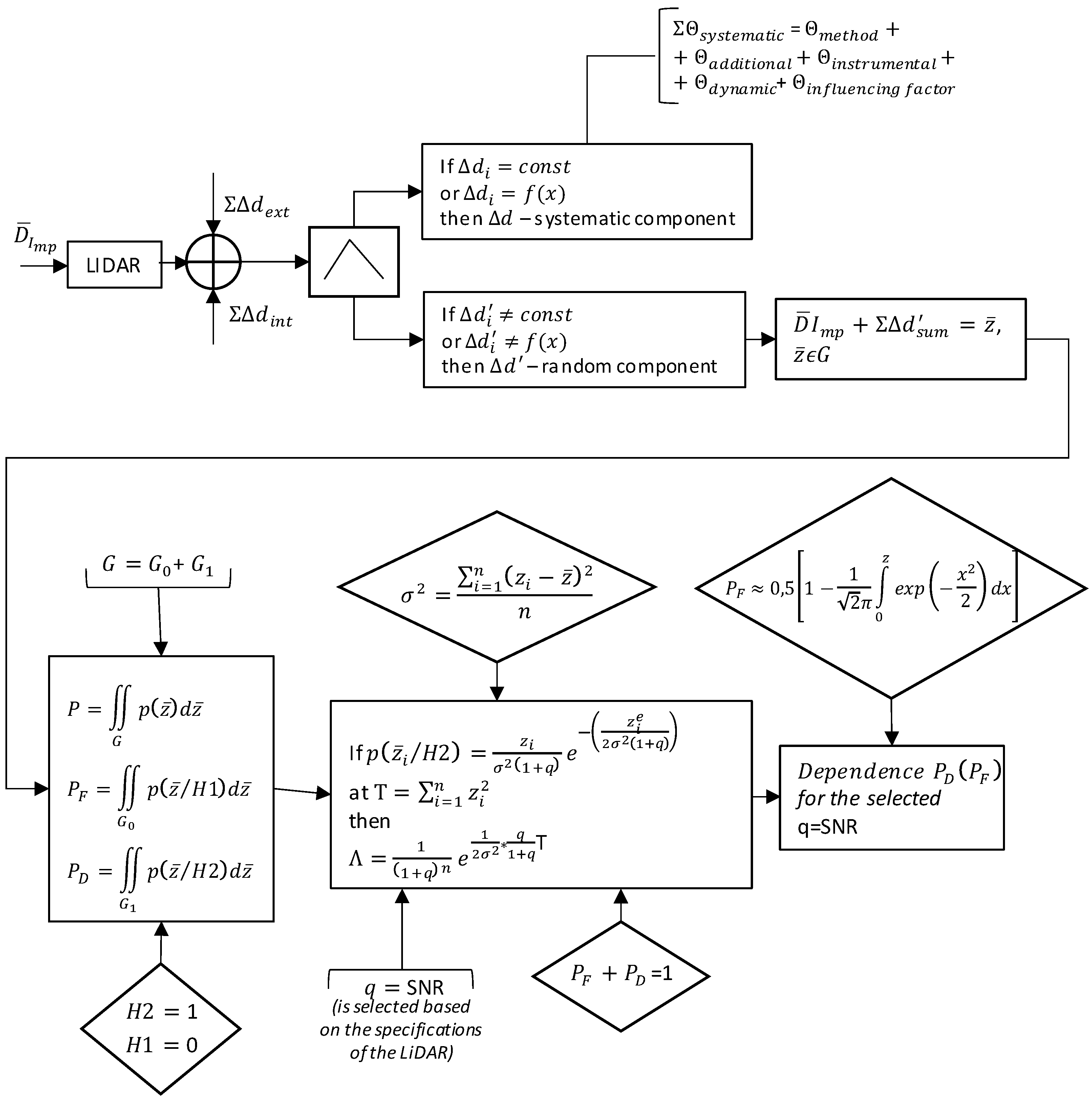
- The detection or extraction of an incoming pulse should be presented as the sum of all return pulses:where DImp—is the generated set of detectable pulses, —the generated set of return pulses from the considered LiDAR;—generated set of pulses from the LiDARs located within reach of each other, as well as multiple pulse re-reflections from objects in space.
- Generate a set of values to assess the probability of “false alarms”:
- Boundary conditions for the interference of re-reflected laser pulses from the considered LiDAR are as follows:
- Boundary conditions for detection (extraction) of the probing pulse from LiDARs located within each other’s range:
where Dr is the generated set of return pulses from the LiDAR for the corresponding set Dinterf; Dinterf is the set of interference pulse values; Dp the set of multiple probing pulses from LiDARs located within range of each other; Q the set of factors contributing the interference of re-reflected impulses; Q′ the set of conditions for detecting probing pulses from LiDARs located within reach of each other. - Definition of the transition matrix for “false event” detection:
- for the interference of re-reflected laser pulses from the considered LiDAR:
- to detect (isolate) a probing pulse from LiDARs located within each other’s range:
where is the set of estimates of the pulse parameter from the considered LiDAR, the set of estimates of pulse parameters from LiDARs located within each other’s range; and the probability of detecting a “false event” for each laser pulse under certain contributing factors and events (if the probability of correct detection of the returning laser pulse is assumed to be 0.95, then the probability of “false events” is 0.05).
6.3. Applying the Approach
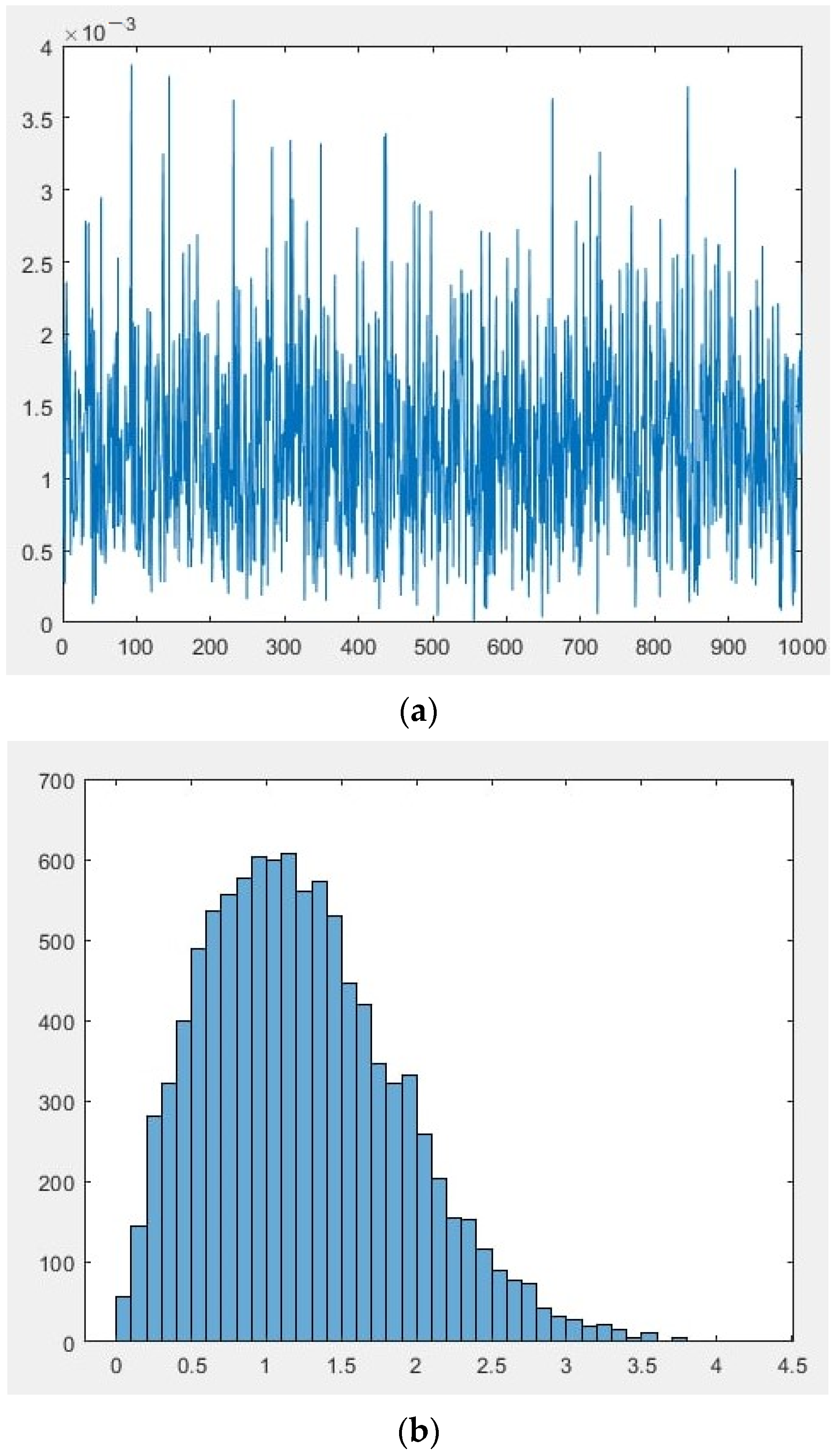
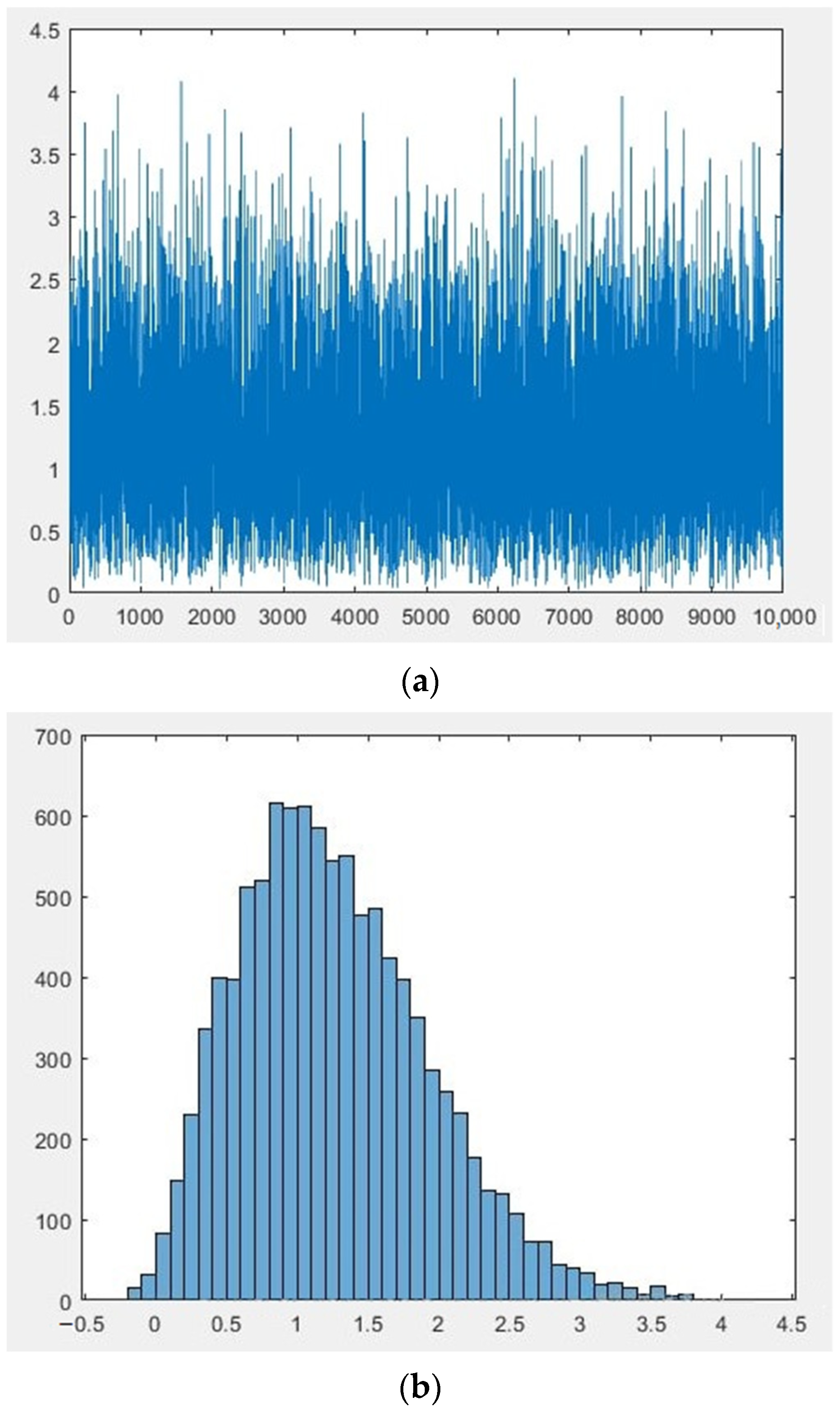
6.4. Generating Datasets for the Research
| Algorithm 1. Finding the dependence of correct signal detection from “false alarms” | |
| Input: (1) the number of observations n; | |
| (2) observation vector // (;); The a priori probabilities of these n observations are unknown. | |
| Output: operating characteristic , i.e., dependence of correct signal detection from “false alarms” with given SNR values for | |
| 1: | // the hypothesis of the reception of a useful signal |
| 2: | // the hypothesis of noise reception |
| 3: | |
| 4: | |
| 5: | |
| 6: | |
| 7: | if then |
| 8: | // probability of error of type I (in which ) |
| 9: | // probability of error of type II (in which ) |
| 10: | for find |
| 11: | for ; findλ |
| 12: | |
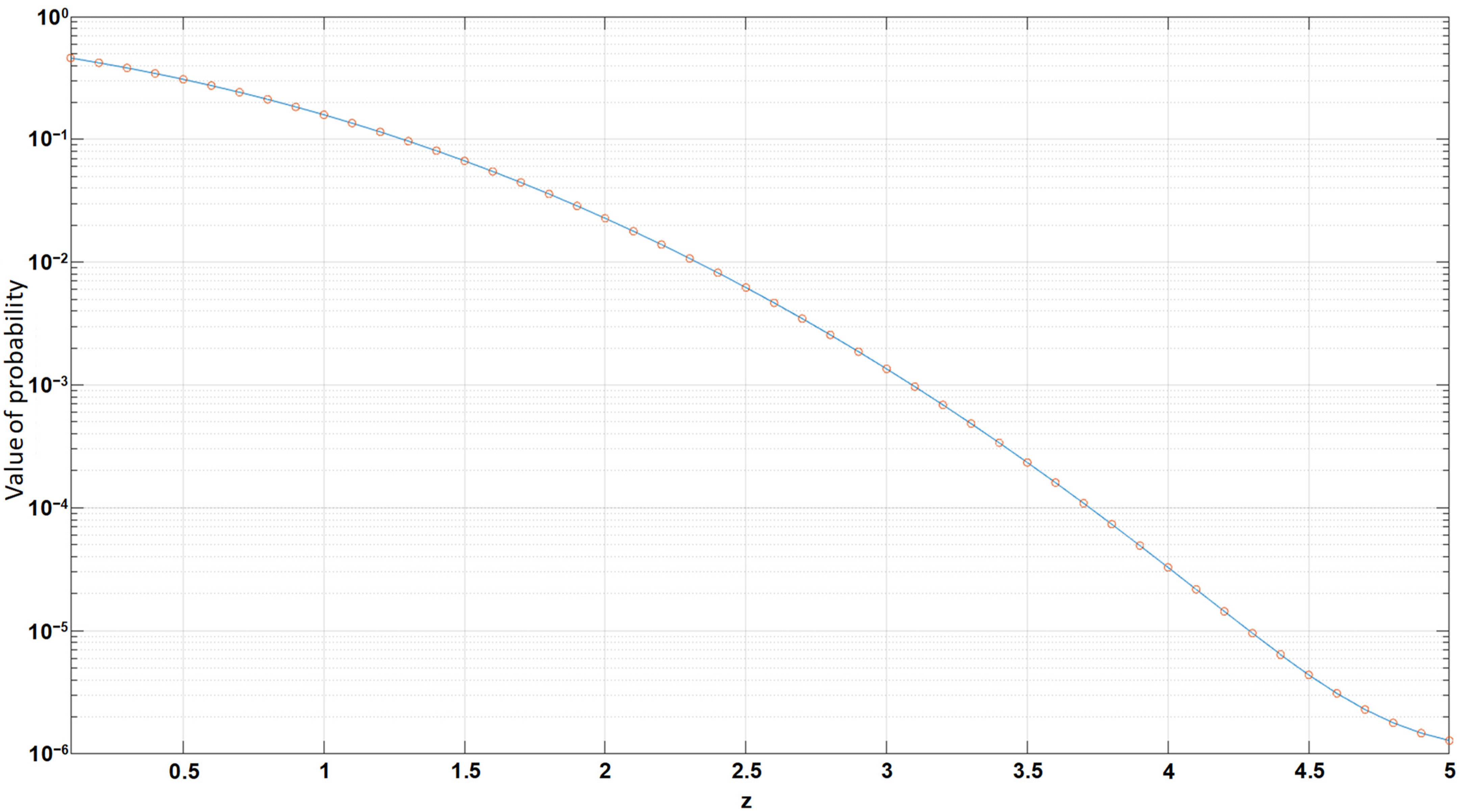
| 13: | for ; find // Rayleigh distribution |
| 14: | plot for ; |
| 15: | end |
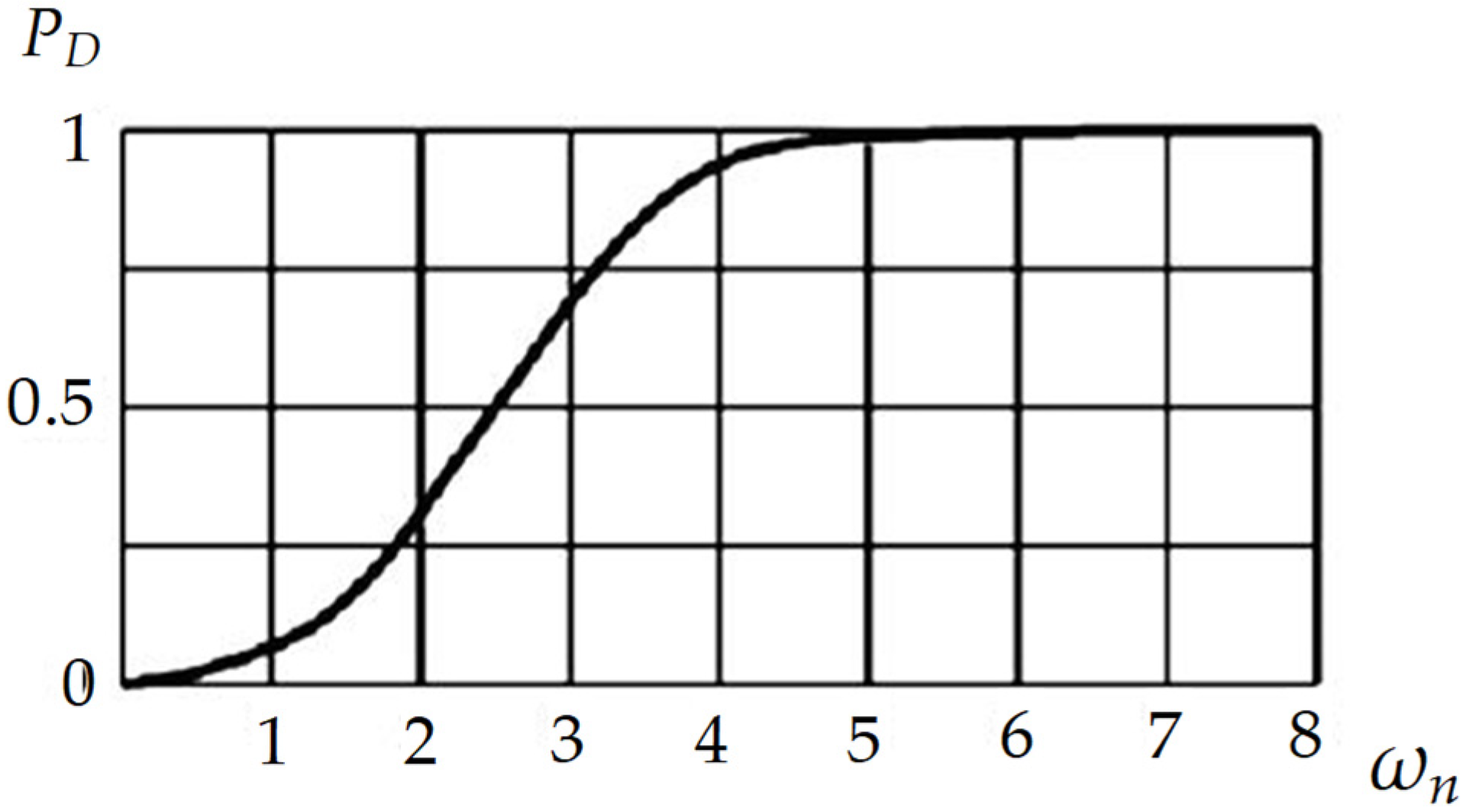
6.5. Plotting the Graph of the Operating Characteristic Depending on the Selected SNR Value
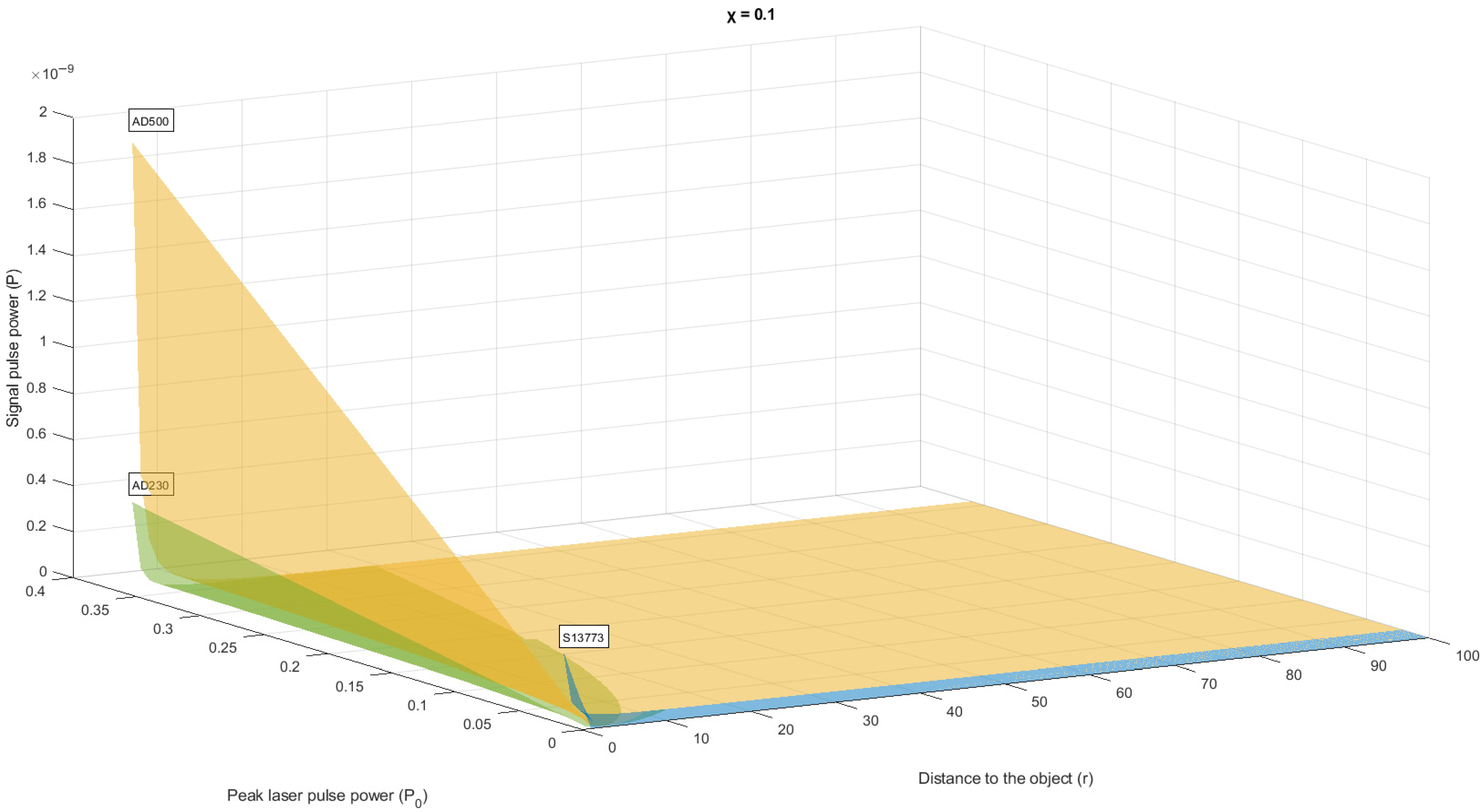
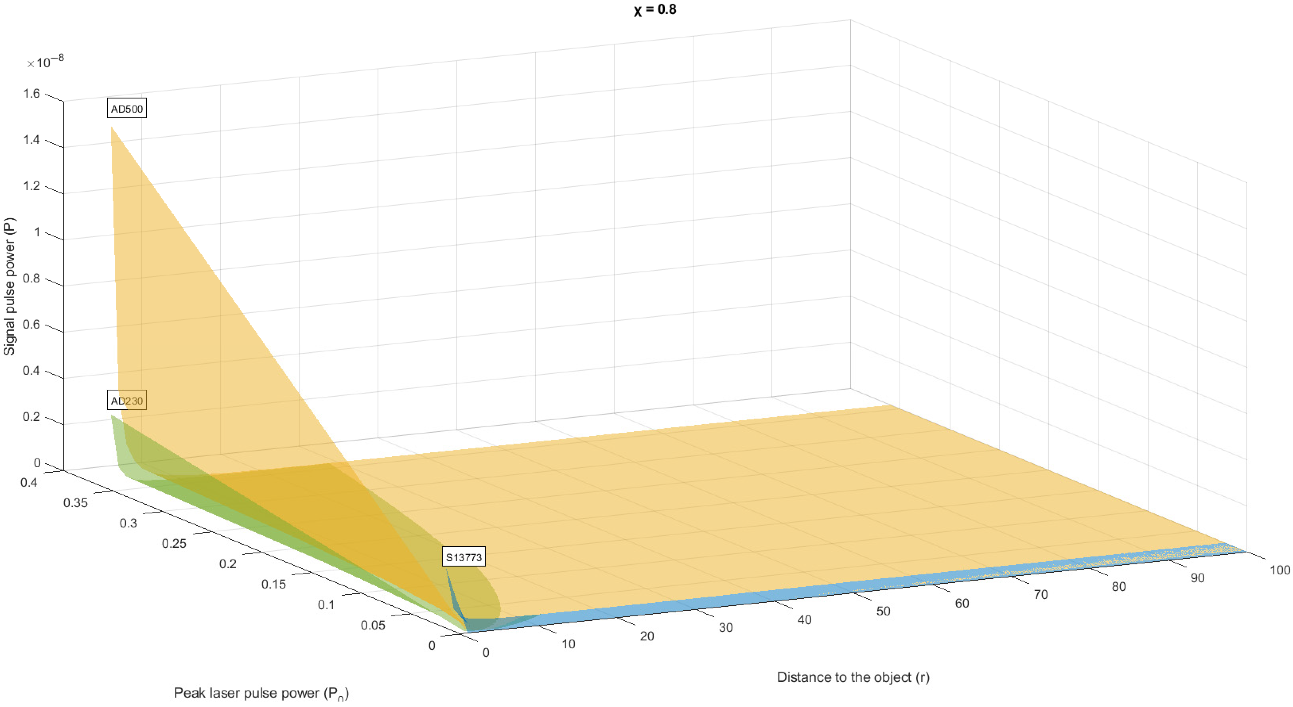
6.6. An Example of Calculating the Received Optical Power of the Photodetectors Based on the Selected SNR Threshold
6.7. Discussion
7. Conclusions
Author Contributions
Funding
Institutional Review Board Statement
Informed Consent Statement
Data Availability Statement
Acknowledgments
Conflicts of Interest
References
- Xu, F.; Xie, Y.; Liu, X.; Chen, X.; Han, W. Research Status and Key Technologies of Intelligent Technology for Unmanned Surface Vehicle System. In Proceedings of the 2020 International Conference on Sensing, Diagnostics, Prognostics, and Control (SDPC), Beijing, China, 5–7 August 2020; pp. 229–233. [Google Scholar]
- Kaligin, N.N.; Uvaysov, S.U.; Uvaysova, A.S.; Uvaysova, S.S. Infrastructural review of the distributed telecommunication system of road traffic and its protocols. Russ. Technol. J. 2019, 7, 87–95. [Google Scholar] [CrossRef]
- Heinzler, R.; Schindler, P.; Seekircher, J.; Ritter, W.; Stork, W. Weather Influence and Classification with Automotive Lidar Sensors. In Proceedings of the 2019 IEEE Intelligent Vehicles Symposium (IV), Paris, France, 9–12 June 2019; pp. 1527–1534. [Google Scholar]
- Lin, S.-L.; Wu, B.-H. Application of Kalman Filter to Improve 3D LiDAR Signals of Autonomous Vehicles in Adverse Weather. Appl. Sci. 2021, 11, 3018. [Google Scholar] [CrossRef]
- Charron, N.; Phillips, S.; Waslander, S.L. De-noising of Lidar Point Clouds Corrupted by Snowfall. In Proceedings of the 2018 15th Conference on Computer and Robot Vision (CRV), Toronto, ON, Canada, 8–10 May 2018; pp. 254–261. [Google Scholar]
- Kunert, M. The EU project MOSARIM: A general overview of project objectives and conducted work. In Proceedings of the 2012 9th European Radar Conference, Amsterdam, The Netherlands, 31 October–2 November 2012; pp. 1–5. [Google Scholar]
- Glennie, C.; Lichti, D.D. Static Calibration and Analysis of the Velodyne HDL-64E S2 for High Accuracy Mobile Scanning. Remote Sens. 2010, 2, 1610–1624. [Google Scholar] [CrossRef] [Green Version]
- Shin, H.; Son, Y.; Park, Y.; Kwon, Y.; Kim, Y. Sampling Race: Bypassing Timing-based Analog Active Sensor Spoofing Detection on Analog-digital Systems. In Proceedings of the 10th USENIX Workshop on Offensive Technologies, Austin, TX, USA, 6–8 August 2016; USENIX Association: Berkeley, CA, USA, 2016; pp. 200–210. [Google Scholar]
- Changalvala, R.; Malik, H. LiDAR Data Integrity Verification for Autonomous Vehicle. IEEE Access 2019, 7, 138018–138031. [Google Scholar] [CrossRef]
- Shin, H.; Kim, D.; Kwon, Y.; Kim, Y. Illusion and Dazzle: Adversarial Optical Channel Exploits Against Lidars for Automotive Applications. In Lecture Notes in Computer Science, Proceedings of the Cryptographic Hardware and Embedded Systems—CHES 2017, Taipei, Taiwan, 25–28 September 2017; Fischer, W., Homma, N., Eds.; Springer: Cham, Switzerland, 2017; Volume 10529, pp. 445–467. [Google Scholar]
- Petit, J.; Stottelaar, B.; Feiri, M. Remote Attacks on Automated Vehicles Sensors: Experiments on Camera and LiDAR. In Proceedings of the Black Hat Europe 2015, Amsterdam, The Netherlands, 10–13 November 2015. [Google Scholar]
- Jagielski, M.; Jones, N.; Lin, C.-W.; Nita-Rotaru, C.; Shiraishi, S. Threat Detection for Collaborative Adaptive Cruise Control in Connected Cars. In Proceedings of the 11th ACM Conference on Security & Privacy in Wireless and Mobile Networks, Stockholm, Sweden, 18–20 June 2018; Association for Computing Machinery: New York, NY, USA, 2018; pp. 184–189. [Google Scholar]
- Bahirat, K.; Prabhakaran, B. A study on LiDAR data forensics. In Proceedings of the 2017 IEEE International Conference on Multimedia and Expo (ICME), Hong Kong, China, 10–14 July 2017; pp. 679–684. [Google Scholar]
- Cao, Y.; Xiao, C.; Cyr, B.; Zhou, Y.; Park, W.; Rampazzi, S.; Chen, Q.A.; Fu, K.; Mao, Z.M. Adversarial Sensor Attack on LiDAR-based Perception in Autonomous Driving. In Proceedings of the 2019 ACM SIGSAC Conference on Computer and Communications Security (CCS’19), London, UK, 11–15 November 2019; Association for Computing Machinery: New York, NY, USA, 2019; pp. 2267–2281. [Google Scholar]
- Stottelaar, B.G. Practical Cyber-Attacks on Autonomous Vehicles. Master’s Thesis, University of Twente, Enschede, The Netherlands, 4 May 2015. [Google Scholar]
- Hau, Z.; Co, K.T.; Demetriou, S.; Lupu, E.C. Object Removal Attacks on LiDAR-based 3D Object Detectors. In Proceedings of the Third International Workshop on Automotive and Autonomous Vehicle Security (AutoSec), San Diego, CA, USA, 25 February 2021; USENIX Association: Berkeley, CA, USA, 2021; pp. 1–4. [Google Scholar]
- Liu, J.; Park, J. “Seeing is not Always Believing”: Detecting Perception Error Attacks against Autonomous Vehicles. IEEE Trans. Dependable Secur. Comput. 2021, 18, 2209–2223. [Google Scholar] [CrossRef]
- Parkinson, S.; Ward, P.; Wilson, K.; Miller, J. Cyber Threats Facing Autonomous and Connected Vehicles: Future Challenges. IEEE Trans. Intell. Transp. Syst. 2017, 18, 2898–2915. [Google Scholar] [CrossRef]
- El-Rewini, Z.; Sadatsharan, K.; Sugunaraj, N.; Selvaraj, D.F.; Plathottam, S.J.; Ranganathan, P. Cybersecurity Attacks in Vehicular Sensors. IEEE Sens. J. 2020, 20, 13752–13767. [Google Scholar] [CrossRef]
- Rivera, S.; Lagraa, S.; Iannillo, A.K.; State, R. Auto-Encoding Robot State against Sensor Spoofing Attacks. In Proceedings of the 2019 IEEE International Symposium on Software Reliability Engineering Workshops (ISSREW), Berlin, Germany, 27–30 October 2019; pp. 252–257. [Google Scholar]
- Sun, J.; Cao, Y.; Chen, Q.A.; Mao, Z.M. Towards Robust LiDAR-based Perception in Autonomous Driving: General Black-box Adversarial Sensor Attack and Countermeasures. In Proceedings of the USENIX Security Symposium, Boston, MA, USA, 12–14 August 2020; USENIX Association: Berkeley, CA, USA, 2020; pp. 1–18. [Google Scholar]
- Chowdhury, A.; Karmakar, G.; Kamruzzaman, J.; Jolfaei, A.; Das, R. Attacks on Self-Driving Cars and Their Countermeasures: A Survey. IEEE Access 2020, 8, 207308–207342. [Google Scholar] [CrossRef]
- Xiang, C.; Qi, C.R.; Li, B. Generating 3d adversarial point clouds. In Proceedings of the 2019 Conference on Computer Vision and Pattern Recognition (CVPR 2019), Long Beach, CA, USA, 16–20 June 2019; pp. 9136–9144. [Google Scholar]
- James, T.; Mengye, R.; Sivabalan, M.; Ming, L.; Bin, Y.; Richard, D.; Frank, C.; Raquel, U. Physically Realizable Adversarial Examples for LiDAR Object Detection. In Proceedings of the 2020 IEEE/CVF Conference on Computer Vision and Pattern Recognition (CVPR 2020), Seattle, WA, USA, 13–19 June 2020; pp. 13713–13722. [Google Scholar]
- Cao, Y.; Xiao, C.; Yang, D.; Fang, J.; Yang, R.; Liu, M.; Li, B. Adversarial objects against LiDAR-based autonomous driving systems. arXiv 2019, arXiv:1907.05418. [Google Scholar]
- Abdelfattah, M.; Yuan, K.; Wang, Z.J.; Ward, R. Adversarial Attacks on Camera-LiDAR Models for 3D Car Detection. In Proceedings of the 2021 Conference on Computer Vision and Pattern Recognition (CVPR 2021), Nashville, TN, USA, 19–25 June 2021; pp. 1–6. [Google Scholar]
- Abdelfattah, M. Adversarial Attacks on Multi-Modal 3D Detection Models. Master’s Thesis, University of British Columbia, Vancouver, BC, Canada, May 2021. [Google Scholar]
- Pham, M.; Xiong, K. A Survey on Security Attacks and Defense Techniques for Connected and Autonomous Vehicles. Comput. Secur. 2021, 109, 102269. [Google Scholar] [CrossRef]
- Liu, Q.; Mo, Y.; Mo, X.; Lv, C.; Mihankhah, E.; Wang, D. Secure Pose Estimation for Autonomous Vehicles under Cyber Attacks. In Proceedings of the 2019 IEEE Intelligent Vehicles Symposium (IV), Paris, France, 9–12 June 2019; pp. 1583–1588. [Google Scholar]
- IEEE Spectrum. Researcher Hacks Self-Driving Car Sensors. Available online: http://spectrum.ieee.org/cars-that-think/transportation/self-driving/researcher-hacks-selfdriving-car-sensors (accessed on 1 July 2021).
- Chan-Tin, E.; Feldman, D.; Hopper, N.; Kim, Y. The Frog-Boiling Attack: Limitations of Anomaly Detection for Secure Network Coordinate Systems. In Lecture Notes of the Institute for Computer Sciences, Social Informatics and Telecommunications Engineering, Proceedings of the Security and Privacy in Communication Networks. SecureComm 2009, Athens, Greece, 14–18 September 2009; Chen, Y., Dimitriou, T.D., Zhou, J., Eds.; Springer: Berlin/Heidelberg, Germany, 2009; Volume 19, pp. 448–458. [Google Scholar]
- Petit, J.; Shladover, S. Potential cyberattacks on automated vehicles. IEEE Trans. Intell. Transp. Syst. 2015, 16, 546–556. [Google Scholar] [CrossRef]
- About Vantablack. Available online: https://www.surreynanosystems.com/about/vantablack (accessed on 1 July 2021).
- Black 3.0—The Blackest Black Paint in the World. Available online: https://www.culturehustleusa.com/products/black-3-0-the-worlds-blackest-black-acrylic-paint-150ml (accessed on 1 July 2021).
- Darkest Manmade Substance. Available online: https://www.guinnessworldrecords.com/world-records/darkest-manmade-substance (accessed on 1 July 2021).
- Blacker Than Black: The First Vantablack Car. Available online: https://www.bmw.com/en/design/the-bmw-X6-vantablack-car.html (accessed on 1 July 2021).
- Rablau, C. LIDAR—A new (self-driving) vehicle for introducing optics to broader engineering and non-engineering audiences. In Proceedings of the Fifteenth Conference on Education and Training in Optics and Photonics (ETOP 2019), Quebec City, QC, Canada, 21–24 May 2019; SPIE: Bellingham, WA, USA, 2019; p. 11143_138. [Google Scholar]
- Monteuuis, J.-P.; Zhang, J.; Mafrica, S.; Servel, A.; Petit, J. Attacker model for Connected and Automated Vehicles. In Proceedings of the ACM Computer Science in Cars Symposium (CSCS 2018), Munich, Germany, 13–14 September 2018; pp. 1–9. [Google Scholar]
- Popko, G.B. Signal Interactions between Lidar Scanners. Available online: https://smartech.gatech.edu/bitstream/handle/1853/62690/POPKO-THESIS-2019.pdf (accessed on 10 November 2021).
- Hwang, I.-P.; Yun, S.-J.; Lee, C.-H. Study on the Frequency-Modulated Continuous-Wave LiDAR Mutual Interference. In Proceedings of the 2019 IEEE 19th International Conference on Communication Technology (ICCT), Xi’an, China, 16–19 October 2019; pp. 1053–1056. [Google Scholar]
- Godbaz, J.P.; Dorrington, A.A.; Cree, M.J. Understanding and Ameliorating Mixed Pixels and Multipath Interference in AMCW Lidar. In TOF Range-Imaging Cameras; Remondino, F., Stoppa, D., Eds.; Springer: Berlin/Heidelberg, Germany, 2013; pp. 91–116. [Google Scholar]
- Kim, G.; Eom, J.; Hur, S.; Park, Y. Analysis on the characteristics of mutual interference between pulsed terrestrial LIDAR scanners. In Proceedings of the 2015 IEEE International Geoscience and Remote Sensing Symposium (IGARSS), Milan, Italy, 26–31 July 2015; pp. 2151–2154. [Google Scholar]
- Kim, G.; Eom, J.; Park, S.; Park, Y. Occurrence and characteristics of mutual interference between LIDAR scanners. In Proceedings of the SPIE, Prague, Czech Republic, 6 May 2015; pp. 1–9. [Google Scholar]
- Kim, G.; Eom, J.; Park, Y. Investigation on the occurrence of mutual interference between pulsed terrestrial LIDAR scanners. In Proceedings of the 2015 IEEE Intelligent Vehicles Symposium (IV), Seoul, Korea, 28 June–1 July 2015; pp. 437–442. [Google Scholar]
- Eom, J.; Kim, G.; Hur, S.; Park, Y. Assessment of Mutual Interference Potential and Impact with off-the-Shelf Mobile LIDAR. In Proceedings of the Bragg Gratings, Photosensitivity and Poling in Glass Waveguides and Materials, Zurich, Switzerland, 2–5 July 2018; Optical Society of America: Washington, DC, USA, 2019; p. JTu2A.66. [Google Scholar]
- Eom, J.; Kim, G.; Park, Y. Mutual interference potential and impact of scanning lidar according to the relevant vehicle applications. In Proceedings of the Laser Radar Technology and Applications XXIV, Baltimore, MD, USA, 2 May 2019; Volume 110050I, pp. 1–10. [Google Scholar]
- Park, Y.; Kim, G.; Eom, J. Design of pulsed scanning lidar without mutual interferences. In Proceedings of the Smart Photonic and Optoelectronic Integrated Circuits XX, San Francisco, CA, USA, 29 January–1 February 2018; Volume 10536, pp. 1–6. [Google Scholar]
- Popko, G.B.; Gaylord, T.K.; Valenta, C.R. Geometric approximation model of inter-lidar interference. Opt. Eng. 2020, 59, 033104. [Google Scholar] [CrossRef]
- Zhang, F.; Du, P.; Liu, Q.; Gong, M.; Fu, X. Adaptive strategy for CPPM single-photon collision avoidance LIDAR against dynamic crosstalk. Opt. Express 2017, 25, 12237–12250. [Google Scholar] [CrossRef] [PubMed]
- Diehm, A.L.; Hammer, M.; Hebel, M.; Arens, M. Mitigation of crosstalk effects in multi-LiDAR configurations. In Proceedings of the Electro-Optical Remote Sensing XII, Berlin, Germany, 9 October 2018; Volume 10796, pp. 1–12. [Google Scholar]
- Wu, J.; Xu, H.; Tian, Y.; Pi, R.; Yue, R. Vehicle Detection under Adverse Weather from Roadside LiDAR Data. Sensors 2020, 20, 3433. [Google Scholar] [CrossRef] [PubMed]
- Kutila, M.; Pyykönen, P.; Ritter, W.; Sawade, O.; Schäufele, B. Automotive LIDAR sensor development scenarios for harsh weather conditions. In Proceedings of the 2016 IEEE 19th International Conference on Intelligent Transportation Systems (ITSC), Rio de Janeiro, Brazil, 1–4 November 2016; pp. 265–270. [Google Scholar]
- Jokela, M.; Pyykönen, P.; Kutila, M.; Kauvo, K. LiDAR Performance Review in Arctic Conditions. In Proceedings of the 2019 IEEE 15th International Conference on Intelligent Computer Communication and Processing (ICCP), Cluj-Napoca, Romania, 5–7 September 2019; pp. 27–31. [Google Scholar]
- Park, J.-I.; Park, J.; Kim, K.-S. Fast and Accurate Desnowing Algorithm for LiDAR Point Clouds. IEEE Access 2020, 8, 160202–160212. [Google Scholar] [CrossRef]
- Ronen, A.; Agassi, E.; Yaron, O. Sensing with Polarized LIDAR in Degraded Visibility Conditions Due to Fog and Low Clouds. Sensors 2021, 21, 2510. [Google Scholar] [CrossRef] [PubMed]
- Vargas Rivero, J.R.; Gerbich, T.; Buschardt, B.; Chen, J. Data Augmentation of Automotive LIDAR Point Clouds under Adverse Weather Situations. Sensors 2021, 21, 4503. [Google Scholar] [CrossRef]
- Trierweiler, M.; Caldelas, P.; Gröninger, G.; Peterseim, T.; Neyman, C. Influence of sensor blockage on automotive LiDAR systems. In Proceedings of the 2019 IEEE SENSORS, Montreal, QC, Canada, 27–30 October 2019; pp. 1–4. [Google Scholar]
- Seo, H.; Yoon, H.; Kim, D.; Kim, J.; Kim, S.-J.; Chun, J.-H.; Choi, J. A 36-Channel SPAD-Integrated Scanning LiDAR Sensor with Multi-Event Histogramming TDC and Embedded Interference Filter. In Proceedings of the 2020 IEEE Symposium on VLSI Circuits, Honolulu, HI, USA, 16–19 June 2020; pp. 1–2. [Google Scholar]
- Carrara, L.; Fiergolski, A. An Optical Interference Suppression Scheme for TCSPC Flash LiDAR Imagers. Appl. Sci. 2019, 9, 2206. [Google Scholar] [CrossRef] [Green Version]
- Hwang, I.-P.; Lee, C.-H. A Rapid LiDAR without Mutual Interferences. In Proceedings of the 2019 Optical Fiber Communications Conference and Exhibition (OFC), San Diego, CA, USA, 3–7 March 2019; pp. 1–3. [Google Scholar]
- Hwang, I.-P.; Lee, C.-H. Mutual Interferences of a True-Random LiDAR with Other LiDAR Signals. IEEE Access 2020, 8, 124123–124133. [Google Scholar] [CrossRef]
- Lei, S.; Yu, S.; Zhang, B.; Wang, G.; Geng, L. A 4-Tap CMOS lock-in modulator with Anti-Interference and Background Canceling for Solid-State Long-Range LiDAR. In Proceedings of the 2019 IEEE International Conference on Electron Devices and Solid-State Circuits (EDSSC), Xi’an, China, 12–14 June 2019; pp. 1–2. [Google Scholar]
- Ximenes, A.R.; Padmanabhan, P.; Lee, M.-J.; Yamashita, Y.; Yaung, D.N.; Charbon, E. A 256 × 256 45/65nm 3D-stacked SPAD-based direct TOF image sensor for LiDAR applications with optical polar modulation for up to 18.6dB interference suppression. In Proceedings of the 2018 IEEE International Solid—State Circuits Conference—(ISSCC), San Francisco, CA, USA, 11–15 February 2018; pp. 96–98. [Google Scholar]
- Chen, Y.; Xie, Y.; Liu, C.; Chen, L. Investigation of Anti-Interference Characteristics of Frequency-Hopping LiDAR. IEEE Photonics Technol. Lett. 2021, 33, 1443–1446. [Google Scholar] [CrossRef]
- Yu, M.; Shi, M.; Hu, W.; Yi, L. FPGA-Based Dual-Pulse Anti-Interference Lidar System Using Digital Chaotic Pulse Position Modulation. IEEE Photonics Technol. Lett. 2021, 33, 757–760. [Google Scholar] [CrossRef]
- Seo, H.; Cho, G.; Kim, J.; Bae, J.; Kim, S.-J.; Chun, J.-H.; Choi, J. A CMOS LiDAR Sensor with Pre-Post Weighted-Histogramming for Sunlight Immunity over 105 klx and SPAD-based Infinite Interference Canceling. In Proceedings of the 2021 Symposium on VLSI Circuits, Kyoto, Japan, 13–19 June 2021; pp. 1–2. [Google Scholar]
- Tsai, C.-M.; Liu, Y.C. Anti-Interference Single-Photon LiDAR Using Stochastic Pulse Position Modulation. Opt. Lett. 2019, 45, 439–442. [Google Scholar] [CrossRef]
- Ishizaki, Y.; Zhang, C.; Set, S.Y.; Yamashita, S. A Novel Software-Based Optical Sampling Scheme for High-Precision and Interference-Free Time-of-Flight LiDAR. In Proceedings of the 2020 Conference on Lasers and Electro-Optics (CLEO), San Jose, CA, USA, 10–15 May 2020; pp. 1–2. [Google Scholar]
- Fersch, T.; Weigel, R.; Koelpin, A. A CDMA Modulation Technique for Automotive Time-of-Flight LiDAR Systems. IEEE Sens. J. 2017, 17, 3507–3516. [Google Scholar] [CrossRef]
- Cheng, C.-H.; Chen, C.-Y.; Chen, J.-D.; Pan, D.-K.; Ting, K.-T.; Lin, F.-Y. 3D pulsed chaos lidar system. Opt. Express 2018, 26, 12230–12241. [Google Scholar] [CrossRef] [PubMed]
- Matsumura, R.; Sugawara, T.; Sakiyama, K. A Secure LIDAR with AES-based Side-Channel Fingerprinting. In Proceedings of the 2018 Sixth International Symposium on Computing and Networking Workshops (CANDARW), Takayama, Japan, 27–30 November 2018; pp. 479–482. [Google Scholar]
- Takefuji, Y. Connected vehicle security vulnerabilities [commentary]. IEEE Technol. Soc. Mag. 2018, 37, 15–18. [Google Scholar] [CrossRef]
- You, C.; Hau, Z.; Demetriou, S. Temporal Consistency Checks to Detect LiDAR Spoofing Attacks on Autonomous Vehicle Perception. In Proceedings of the 1st Workshop on Security and Privacy for Mobile AI (MAISP’21), Virtual, 25 June 2021; pp. 13–18. [Google Scholar]
- Boreysho, A.S.; Kim, A.A.; Konyaev, M.A.; Luginya, V.S.; Morozov, A.V.; Orlov, A.E. Modern Lidar Systems for Atmosphere Remote Sensing. Photonics Russia 2019, 7, 648–657. [Google Scholar]


| Symbol | Characteristic | Test Condition | Value | Unit |
|---|---|---|---|---|
| “First Sensor” | ||||
| AD230-9 SMD; AD230-9 TO | ||||
| Active area | 0.04 | mm2 | ||
| Responsivity | M = 100; λ = 905 nm | 52; 58; 60 | A/W | |
| Quantum efficiency | λ: 750–905 nm | 80 | % | |
| IPEAK | Peak DC current | 0.25 | mA | |
| ID | Dark current | M = 100 | 0.5 | nA |
| AD500-9 SMD | ||||
| Active area | 0.196 | mm2 | ||
| Responsivity | M = 100; λ = 905 nm | 52; 58; 60 | A/W | |
| Quantum efficiency | λ: 750–905 nm | 80 | % | |
| IPEAK | Peak DC current | 0.25 | mA | |
| ID | Dark current | M = 100 | 0.8 | nA |
| AD500-9-400M TO5 | ||||
| Active area | 0.196 | mm2 | ||
| Responsivity | M = 100; λ = 905 nm | 52; 58; 60 | A/W | |
| Quantum efficiency | λ: 750–910 nm | 80 | % | |
| IPEAK | Peak DC current | 0.63 | mA | |
| ID | Dark current | M = 100 | 0.8 | nA |
| “Hamamatsu” | ||||
| Si PIN photodiodes S13773 and S15193 | ||||
| Active area | 0.5 | mm2 | ||
| Responsivity | M = 100 | 0.54; 0.64 | A/W | |
| Quantum efficiency | λ: 785 nm; 830 nm | 80 | % | |
| IPEAK | Peak DC current | 0.1; 0.3 | mA | |
| ID | Dark current | M = 100 | 10 | nA |
Publisher’s Note: MDPI stays neutral with regard to jurisdictional claims in published maps and institutional affiliations. |
© 2022 by the authors. Licensee MDPI, Basel, Switzerland. This article is an open access article distributed under the terms and conditions of the Creative Commons Attribution (CC BY) license (https://creativecommons.org/licenses/by/4.0/).
Share and Cite
Meshcheryakov, R.; Iskhakov, A.; Mamchenko, M.; Romanova, M.; Uvaysov, S.; Amirgaliyev, Y.; Gromaszek, K. A Probabilistic Approach to Estimating Allowed SNR Values for Automotive LiDARs in “Smart Cities” under Various External Influences. Sensors 2022, 22, 609. https://doi.org/10.3390/s22020609
Meshcheryakov R, Iskhakov A, Mamchenko M, Romanova M, Uvaysov S, Amirgaliyev Y, Gromaszek K. A Probabilistic Approach to Estimating Allowed SNR Values for Automotive LiDARs in “Smart Cities” under Various External Influences. Sensors. 2022; 22(2):609. https://doi.org/10.3390/s22020609
Chicago/Turabian StyleMeshcheryakov, Roman, Andrey Iskhakov, Mark Mamchenko, Maria Romanova, Saygid Uvaysov, Yedilkhan Amirgaliyev, and Konrad Gromaszek. 2022. "A Probabilistic Approach to Estimating Allowed SNR Values for Automotive LiDARs in “Smart Cities” under Various External Influences" Sensors 22, no. 2: 609. https://doi.org/10.3390/s22020609