
Deployment and Allocation Strategy for MEC Nodes in Complex Multi-Terminal Scenarios

Abstract
:1. Introduction
- We design a model for complex terminal application scenarios. By analyzing the characteristics of terminal emergency and power supply modes, the model is suitable for specific application scenarios. We consider the processing capability of edge nodes and ultimately select suitable nodes among several potential edge nodes.
- An improved genetic algorithm (GA) is designed and compared with the k-means and ant colony (ACO) algorithms. We analyze the advantages and disadvantages of the three algorithms in terms of the iterative process, task assignment balance, and final optimization results. GA achieves the best performance; therefore, it is used to test different terminal attributes.
- We test the performance of the algorithm under different scenarios and analyze its applicability under varying terminal and edge node sparsity conditions, task flow rates, data volume ranges, and task processing complexities, providing a reference for subsequent application studies to explore additional scenarios.
2. Literature Review
3. System Model
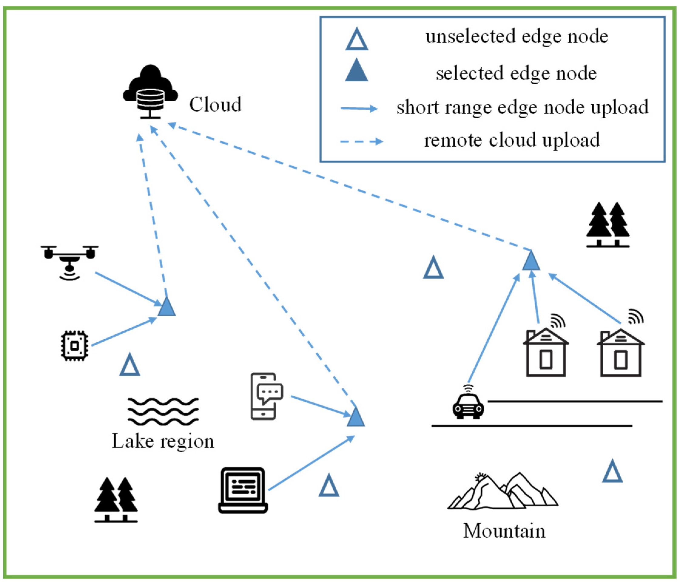
3.1. Scenario Description
- Urgency : In the actual scenario, different locations correspond to terminals with different requirements for time tolerance sensitivity, so we divide terminals into three levels of urgency , with as the most urgent terminal and as the least urgent terminal. During processing, tasks created by high-urgency terminals have a preference with respect to the degree of reward, as specifically described in Section 3.2.2.
- Task complexity : Task complexity affects the amount of CPU time spent on task processing. The higher the complexity of the task, the longer the processing time. For example, edge nodes consume more computational resources than text processing when dealing with image-type tasks. In this paper, we consider four common task types: ASCII compression, data table reading, variable-bit-rate (VBR) coding, and constant-bit-rate (CBR) coding, with a complexity of y of 330 cycles/byte, 960 cycles/byte, 1300 cycles/byte, and 1900 cycles/byte, respectively [24].
- Task rate : indicates the number of tasks generated by terminal per unit of time, where the task-generated rate () by terminals obeys the Poisson distribution.
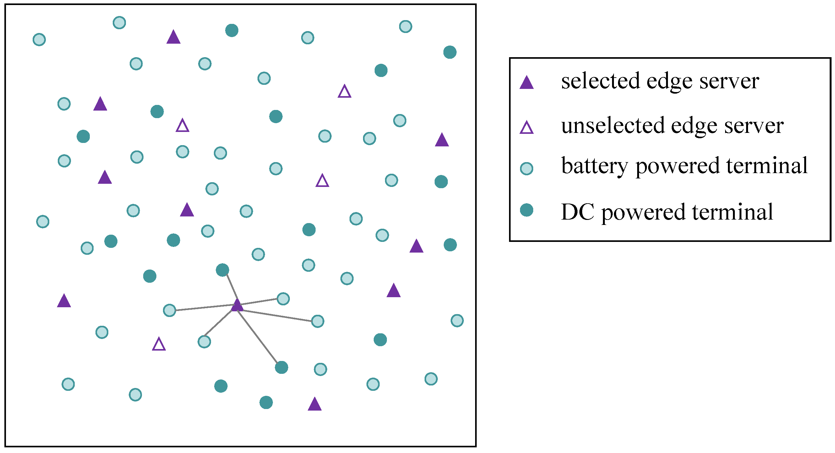
- Power supply modes : Each terminal device has two power supply modes, i.e., battery-powered (harsh environment, unable to meet the conditions of the external power supply) or direct power supply. In particular, only one of the two power supply modes is available for each terminal. Thus, the power supply method of the terminal can be expressed as Equation (1). means that the terminal is powered by a battery, whereas means that the terminal is powered by DC. and indicate the energy consumption weights of the two power supply modes. In Figure 2, the dark green and light green circles represent different power supply modes of terminals.
3.2. Optimization Function Design
3.2.1. Optimization Function
3.2.2. Influencing Factor of Reward
- 1.
- Transmission latency
- 2.
- Queuing latency
- 3.
- Processing latency
3.2.3. Influencing Factor of Battery Power
3.2.4. Influencing Factor of Deployment Cost
3.2.5. Performance Metrics
- 1.
- Latency
- 2.
- Deployment balance
4. Description of Algorithms
4.1. k-Means
| Algorithm 1: k-means for the Placement Scheme |
| Input: , , Number of cluster k |
| Output: , |
| Randomly select k points as the starting center |
| Do: |
| Set by |
| While changes |
| Find by minimal |
| Calculate |
4.2. ACO
| Algorithm 2: ACO for the Placement Scheme |
| Input: , |
| Output: , |
| , |
| While |
| Initial |
| End |
| While |
| Foreach do |
| Create by |
| Get & |
| End |
| End |
| Find by |
| Calculate |
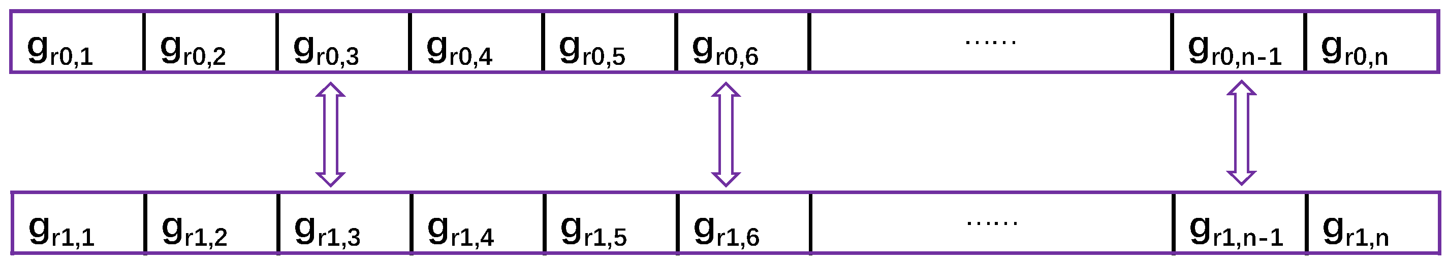
4.3. GA
- 1.
- Selection of parents
- 2.
- Crossing
- 3.
- Mutation
- 4.
- Generation of new populations
| Algorithm 3: GA for the Placement Scheme |
| Input: , |
| Output: , |
| , |
| While |
| Initial |
| End |
| While |
| Sort by |
| While parents do |
| Select parents & by |
| Apply crossing to get offspring & |
| Apply mutation to & |
| End |
| Sort for finding |
| End |
| Find by |
| Calculate |
5. Results
5.1. Experimental Conditions
5.2. Results Analysis
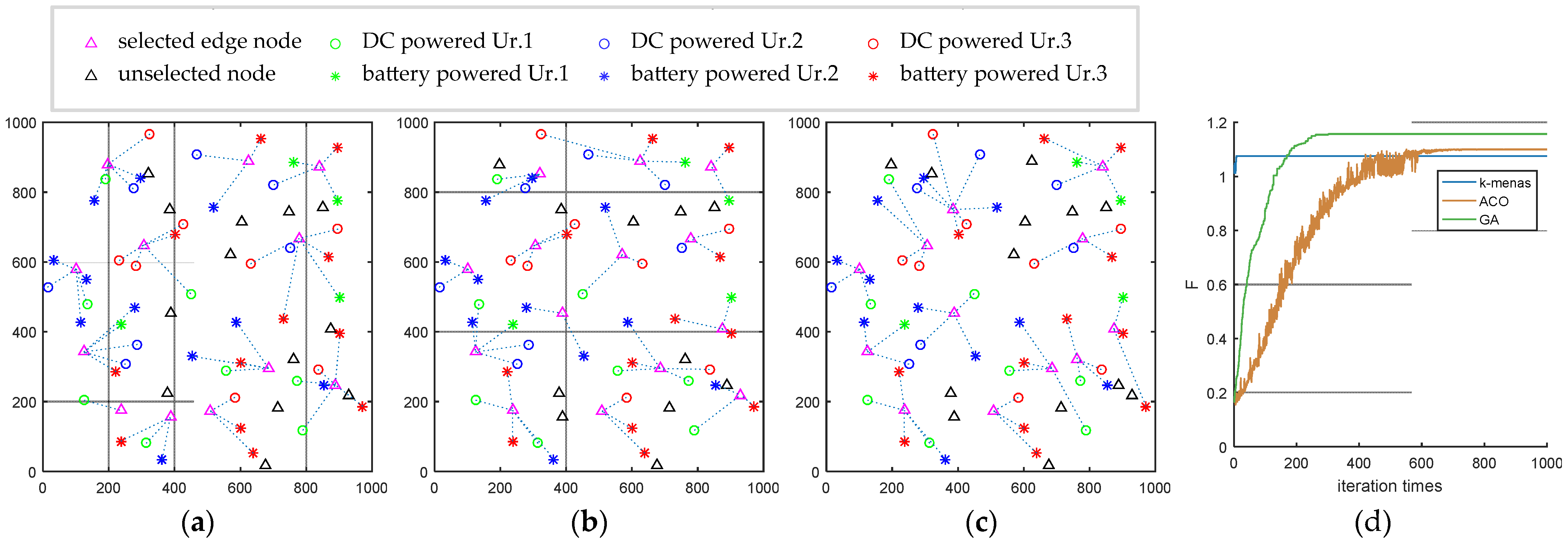
5.2.1. Comparison of Three Algorithms
5.2.2. Four Parameter Changes for the Investigated Scenario
- 1.
- Changing the number of edge nodes and terminals
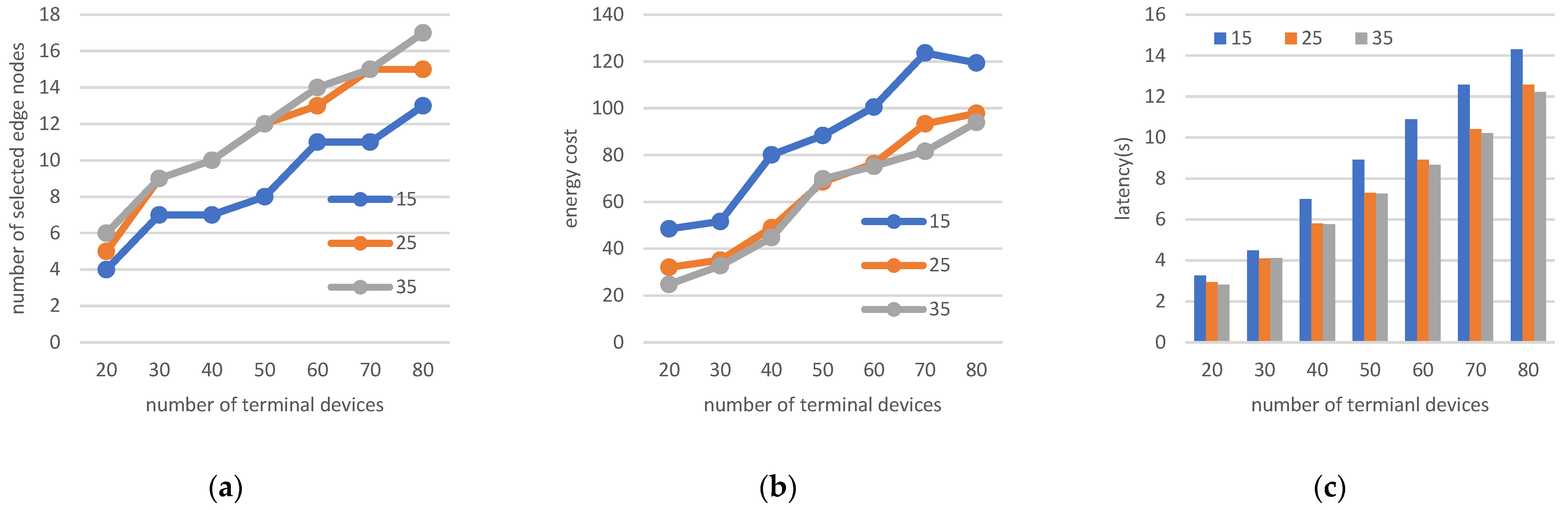
- 2.
- Changing the number of terminals and node processing capacity
- 3.
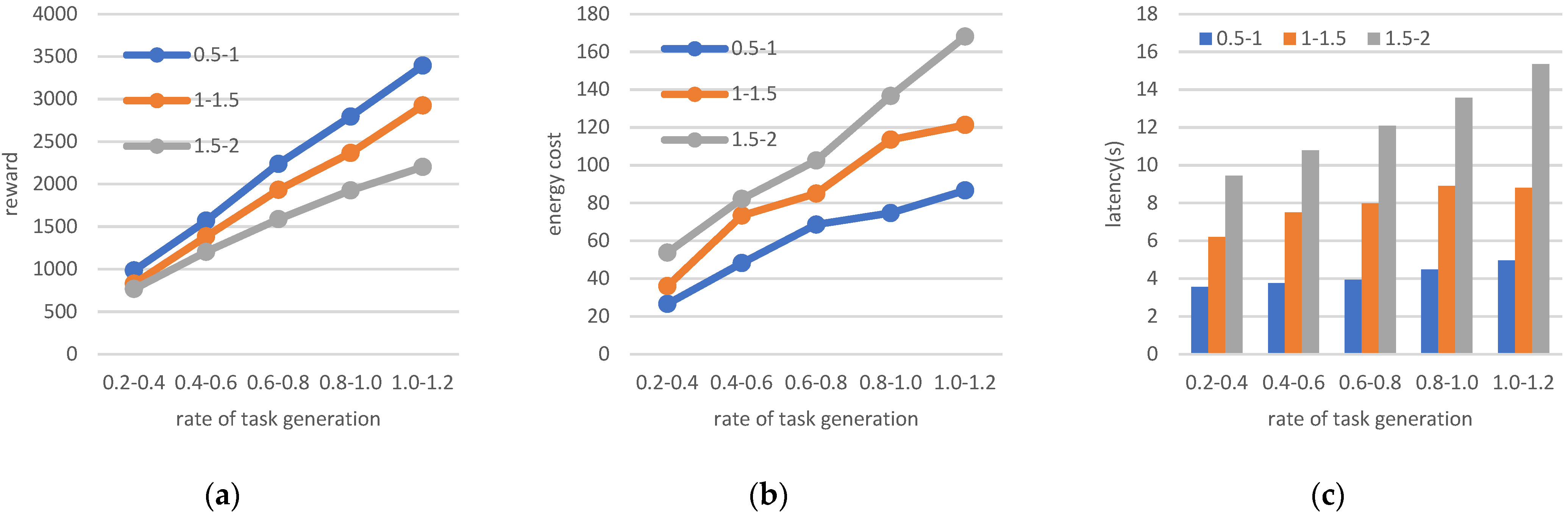
- Changing the amount of data and generated task rate
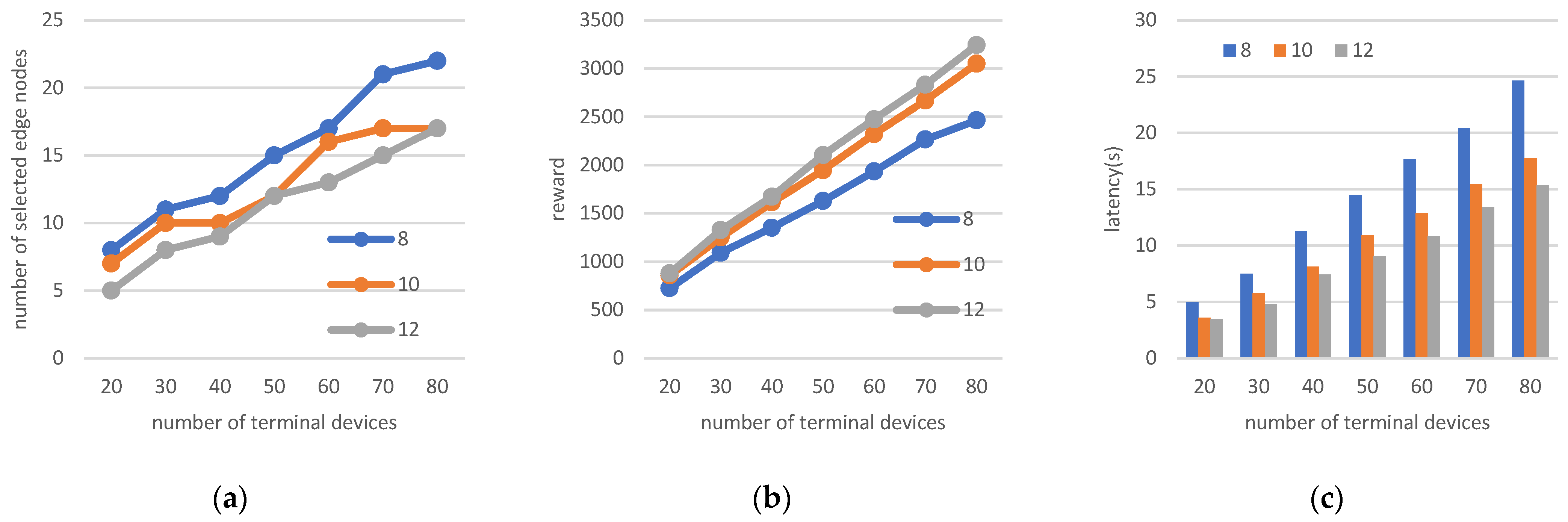
- 4.
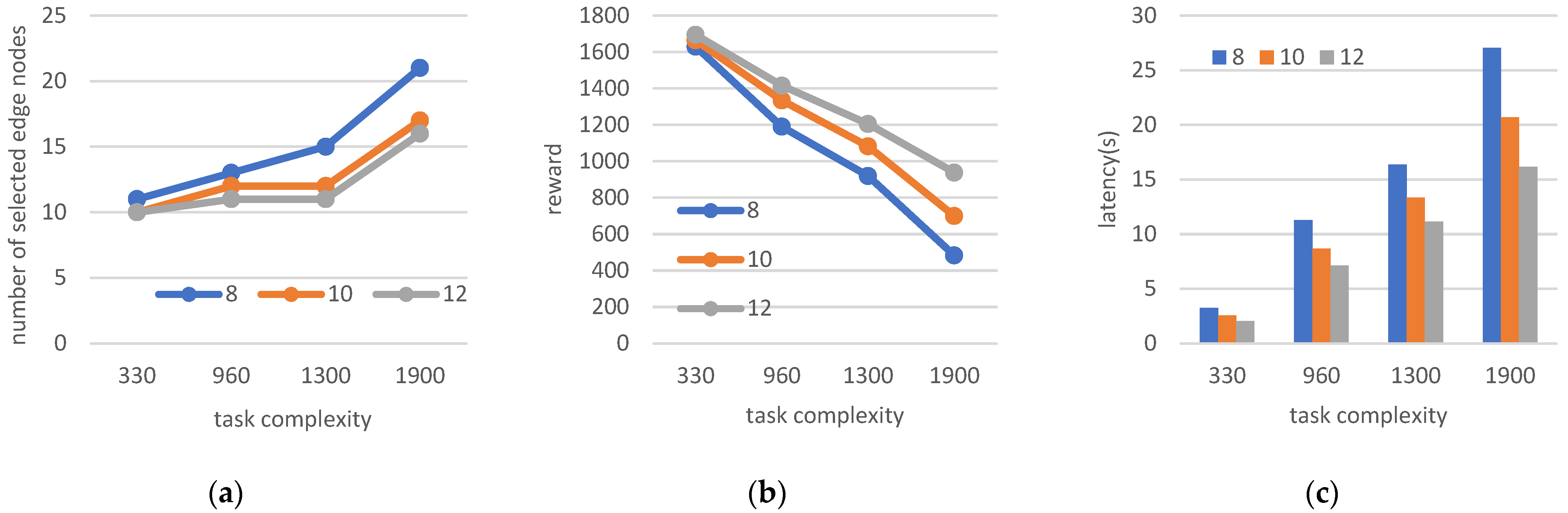
- Changing task complexity and edge node processing capability;
6. Conclusions and Future Work
- The current complex actual deployment scenario involves more requirements with respect to the service types of edge node task processing, and we hope to add planning for the services of edge nodes in conjunction with the deployment strategy in the future.
- Using a machine learning approach to strategic allocation for edge node selection can improve efficiency and simplify planning [31].
- In response to the increase in the number of terminals and the change in data, we will introduce more parameter settings that match the actual situation, fully consider the nonlinear relationship between generated task data volume and task complexity, and design a more scientific and complete system cost model.
- Due to the variety of mobile edge node applications, subsequent work should consider a dynamic edge node deployment strategy.
Author Contributions
Funding
Institutional Review Board Statement
Informed Consent Statement
Data Availability Statement
Conflicts of Interest
References
- Zhang, C.; Patras, P.; Haddadi, H. Deep learning in mobile and wireless networking: A survey.IEEE. Commun. Surv. Tutor. 2019, 21, 2224–2287. [Google Scholar] [CrossRef]
- Paśko, Ł.; Mądziel, M.; Stadnicka, D.; Dec, G.; Carreras-Coch, A.; Solé-Beteta, X.; Pappa, L.; Stylios, C.; Mazzei, D.; Atzeni, D. Plan and Develop Advanced Knowledge and Skills for Future Industrial Employees in the Field of Artificial Intelligence, Internet of Things and Edge Computing. Sustainability 2022, 14, 3312. [Google Scholar] [CrossRef]
- Dec, G.; Stadnicka, D.; Paśko, Ł.; Mądziel, M.; Figliè, R.; Mazzei, D.; Tyrovolas, M.; Stylios, C.; Navarro, J.; Solé-Beteta, X. Role of Academics in Transferring Knowledge and Skills on Artificial Intelligence, Internet of Things and Edge Computing. Sensors 2022, 22, 2496. [Google Scholar] [CrossRef] [PubMed]
- Smolka, S.; Mann, Z.Á. Evaluation of fog application placement algorithms: A survey. Computing 2022, 342, 1–27. [Google Scholar] [CrossRef]
- Mao, Y.; You, C.; Zhang, J.; Huang, K.; Letaief, K.B. A survey on mobile edge computing: The communication perspective. IEEE Commun. Surv. Tutor. 2017, 19, 2322–2358. [Google Scholar] [CrossRef]
- Sonkoly, B.; Czentye, J.; Szalay, M.; Németh, B.; Toka, L. Survey on Placement Methods in the Edge and Beyond. IEEE Commun. Surv. Tutor. 2021, 23, 2590–2629. [Google Scholar] [CrossRef]
- Salaht, F.A.; Desprez, F.; Lebre, A. An overview of service placement problem in fog and edge computing. ACM Comput. Surv. (CSUR) 2020, 53, 1–35. [Google Scholar] [CrossRef]
- Rodrigues, T.K.; Suto, K.; Nishiyama, H.; Liu, J.; Kato, N. Machine learning meets computation and communication control in evolving edge and cloud: Challenges and future perspective. IEEE Commun. Surv. Tutor. 2019, 22, 38–67. [Google Scholar] [CrossRef]
- Almajali, S.; Abou-Tair, D.e.D.I.; Salameh, H.B.; Ayyash, M.; Elgala, H. A distributed multi-layer MEC-cloud architecture for processing large scale IoT-based multimedia applications. Multimed. Tools Appl. 2019, 78, 24617–24638. [Google Scholar] [CrossRef]
- Zhang, J.; Li, M.; Zheng, X.; Hsu, C.H. A Time-Driven Cloudlet Placement Strategy for Workflow Applications in Wireless Metropolitan Area Networks. Sensors 2022, 22, 3422. [Google Scholar] [CrossRef]
- Lähderanta, T.; Leppänen, T.; Ruha, L.; Lovén, L.; Harjula, E.; Ylianttila, M.; Riekki, J.; Sillanpää, M.J. Edge computing server placement with capacitated location allocation. J. Parallel Distrib. Comput. 2021, 153, 130–149. [Google Scholar] [CrossRef]
- Gupta, D.; Kuri, J. Optimal Network Design: Edge Server Placement and Link Capacity Assignment for Delay-Constrained Services. In Proceedings of the 2021 17th International Conference on Network and Service Management (CNSM), IEEE, Izmir, Turkey, 25–29 October 2021; pp. 111–117. [Google Scholar]
- Jabri, I.; Mekki, T.; Rachedi, A.; Jemaa, M.B. Vehicular fog gateways selection on the internet of vehicles: A fuzzy logic with ant colony optimization based approach. Ad Hoc Netw. 2019, 91, 101879. [Google Scholar] [CrossRef]
- Chang, L.; Deng, X.; Pan, J.; Zhang, Y. Edge Server Placement for Vehicular Ad Hoc Networks in Metropolitans. IEEE Internet Things J. 2022, 9, 1575–1590. [Google Scholar] [CrossRef]
- Jiang, C.; Wan, J.; Abbas, H. An edge computing node deployment method based on improved k-means clustering algorithm for smart manufacturing. IEEE Syst. J. 2020, 15, 2230–2240. [Google Scholar] [CrossRef]
- Wang, Z.; Zhang, W.; Jin, X.; Huang, Y.; Lu, C. An optimal edge server placement approach for cost reduction and load balancing in intelligent manufacturing. J. Supercomput. 2022, 78, 4032–4056. [Google Scholar] [CrossRef]
- Cao, K.; Li, L.; Cui, Y.; Wei, T.; Hu, S. Exploring Placement of Heterogeneous Edge Servers for Response Time Minimization in Mobile Edge-Cloud Computing. IEEE Trans. Ind. Inform. 2021, 17, 494–503. [Google Scholar] [CrossRef]
- Lin, C.C.; Yang, J.W. Cost-efficient deployment of fog computing systems at logistics centers in industry 4.0. IEEE Trans. Ind. Inform. 2018, 14, 4603–4611. [Google Scholar] [CrossRef]
- Jia, M.; Cao, J.; Liang, W. Optimal Cloudlet Placement and User to Cloudlet Allocation in Wireless Metropolitan Area Networks. IEEE Trans. Cloud Comput. 2015, 5, 725–737. [Google Scholar] [CrossRef]
- Luo, F.; Zheng, S.; Ding, W.; Fuentes, J.; Li, Y. An Edge Server Placement Method Based on Reinforcement Learning. Entropy 2022, 24, 317. [Google Scholar] [CrossRef]
- Mann, Z.A. Decentralized application placement in fog computing. IEEE Trans. Parallel Distrib. Syst. 2022, 33, 3262–3273. [Google Scholar] [CrossRef]
- Herrera, J.L.; Galán-Jiménez, J.; Foschini, L.; Bellavista, P.; Berrocal, J.; Murillo, J.M. QoS-Aware Fog Node Placement for Intensive IoT Applications in SDN-Fog Scenarios. IEEE Internet Things J. 2022, 9, 13725–13739. [Google Scholar] [CrossRef]
- Zhao, L.; Li, B.; Tan, W.; Cui, G.; He, Q.; Xu, X.; Xu, L.; Yang, Y. Joint Coverage-Reliability for Budgeted Edge Application Deployment in Mobile Edge Computing Environment. IEEE Trans. Parallel Distrib. Syst. 2022, 33, 3760–3771. [Google Scholar] [CrossRef]
- Miettinen, A.P.; Nurminen, J.K. Energy efficiency of mobile clients in cloud computing. In Proceedings of the 2nd USENIX Workshop on Hot Topics in Cloud Computing (HotCloud 10), Boston, MA, USA, 22 June 2010; pp. 1–7. [Google Scholar]
- Heinzelman, W.B.; Chandrakasan, A.P.; Balakrishnan, H. An application-specific protocol architecture for wireless microsensor networks. IEEE Trans. Wirel. Commun. 2002, 1, 660–670. [Google Scholar] [CrossRef]
- Ei, N.N.; Kang, S.W.; Alsenwi, M.; Tun, Y.K.; Hong, C.S. Multi-UAV-Assisted MEC System: Joint Association and Resource Management Framework. In Proceedings of the 2021 International Conference on Information Networking (ICOIN), Jeju Island, Korea, 13–16 January 2021; pp. 213–218. [Google Scholar]
- Singh, P.; Dutta, M.; Aggarwal, N. A review of task scheduling based on meta-heuristics approach in cloud computing. Knowl. Inf. Syst. 2017, 52, 1–51. [Google Scholar] [CrossRef]
- Somesula, M.K.; Rout, R.R.; Somayajulu, D.V. Contact duration-aware cooperative cache placement using genetic algorithm for mobile edge networks. Comput. Netw. 2021, 193, 108062. [Google Scholar] [CrossRef]
- Huang, L.; Bi, S.; Zhang, Y.J.A. Deep reinforcement learning for online computation offloading in wireless powered mobile-edge computing networks. IEEE Trans. Mob. Comput. 2019, 19, 2581–2593. [Google Scholar] [CrossRef]
- Zhao, H.; Mao, Y.; Cheng, T. Study on the transmission path and timing scheduling for WSNs with heterogeneous nodes. Sens. Rev. 2018, 39, 51–57. [Google Scholar] [CrossRef]
- Gill, S.S.; Xu, M.; Ottaviani, C.; Patros, P.; Bahsoon, R.; Shaghaghi, A.; Golec, M.; Stankovski, V.; Wu, H.; Abraham, A.; et al. AI for next generation computing: Emerging trends and future directions. Internet Things 2022, 19, 100514. [Google Scholar] [CrossRef]


| Reference | Terminal Attributes | Evaluations | |||||
|---|---|---|---|---|---|---|---|
| Data | Task Flow Rate | Power Supply Mode | Urgency | Edge Node Number | Energy Consumption | Latency | |
| This paper | √ | √ | √ | √ | √ | √ | √ |
| [14] | √ | × | × | × | √ | × | √ |
| [18] | √ | √ | × | × | √ | × | √ |
| [16] | √ | √ | √ | × | √ | √ | √ |
| [15] | √ | √ | √ | × | × | √ | √ |
| [17] | √ | × | × | × | √ | × | √ |
| Notation | Details |
|---|---|
| [20, 80] | |
| [10, 40] | |
| 1 | |
| 0.2 | |
| [1, 2, 3] | |
| 1 | |
| [0.2–1.2] | |
| [330, 960, 1300, 1900, 2100] cycles/byte | |
| [0.5–2] MB | |
| 8 MB | |
| 500 m | |
| [8, 10, 12] GHz | |
| 1, 1, 1.3 | |
| 50, 100, 1 |
| Notation | Details |
|---|---|
| 1000 | |
| 400 | |
| 1 | |
| 0.7 | |
| 400 | |
| 0.9 | |
| 0.05 |
| Algorithm | Number of Edge Nodes | Latency | Run Time | Variance | |||
|---|---|---|---|---|---|---|---|
| k-means | 1.075 | 1834.894 | 67.494 | 12 | 5.749 | 0.883 | 0.441 |
| ACO | 1.099 | 1854.426 | 54.580 | 14 | 5.463 | 46.574 | 0.390 |
| GA | 1.156 | 1842.622 | 63.005 | 12 | 5.637 | 13.918 | 0.282 |
Publisher’s Note: MDPI stays neutral with regard to jurisdictional claims in published maps and institutional affiliations. |
© 2022 by the authors. Licensee MDPI, Basel, Switzerland. This article is an open access article distributed under the terms and conditions of the Creative Commons Attribution (CC BY) license (https://creativecommons.org/licenses/by/4.0/).
Share and Cite
Li, D.; Mao, Y.; Chen, X.; Li, J.; Liu, S. Deployment and Allocation Strategy for MEC Nodes in Complex Multi-Terminal Scenarios. Sensors 2022, 22, 6719. https://doi.org/10.3390/s22186719
Li D, Mao Y, Chen X, Li J, Liu S. Deployment and Allocation Strategy for MEC Nodes in Complex Multi-Terminal Scenarios. Sensors. 2022; 22(18):6719. https://doi.org/10.3390/s22186719
Chicago/Turabian StyleLi, Danyang, Yuxing Mao, Xueshuo Chen, Jian Li, and Siyang Liu. 2022. "Deployment and Allocation Strategy for MEC Nodes in Complex Multi-Terminal Scenarios" Sensors 22, no. 18: 6719. https://doi.org/10.3390/s22186719