
Distance- and Momentum-Based Symbolic Aggregate Approximation for Highly Imbalanced Classification

Abstract
:1. Introduction
2. Related Works
2.1. Conventional SAX
2.2. Real-World Applications of SAX
2.3. Variations of SAX
3. Proposed Method: DM-SAX
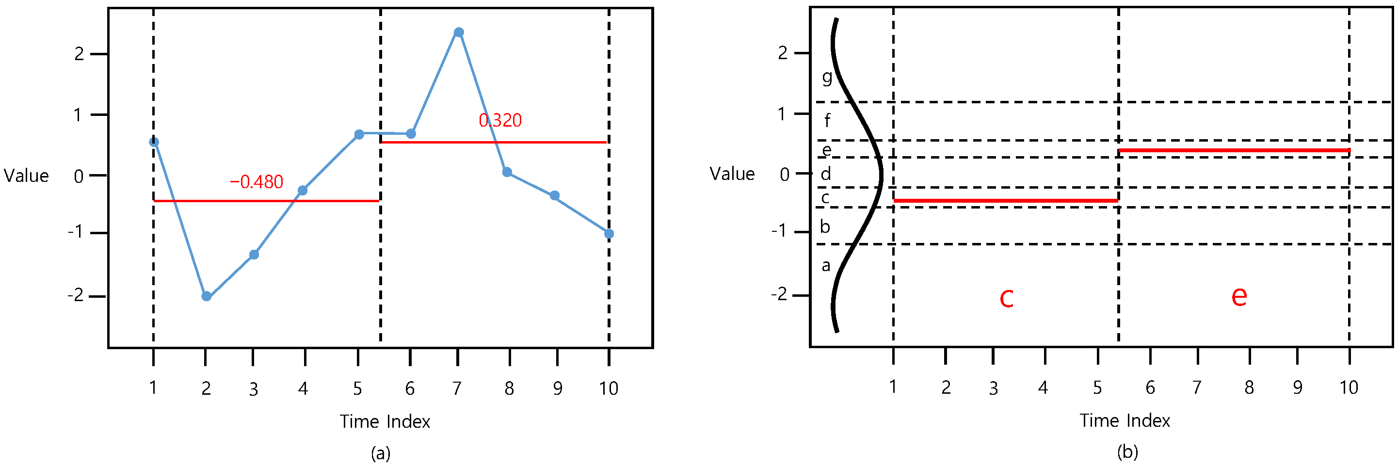
3.1. D-SAX
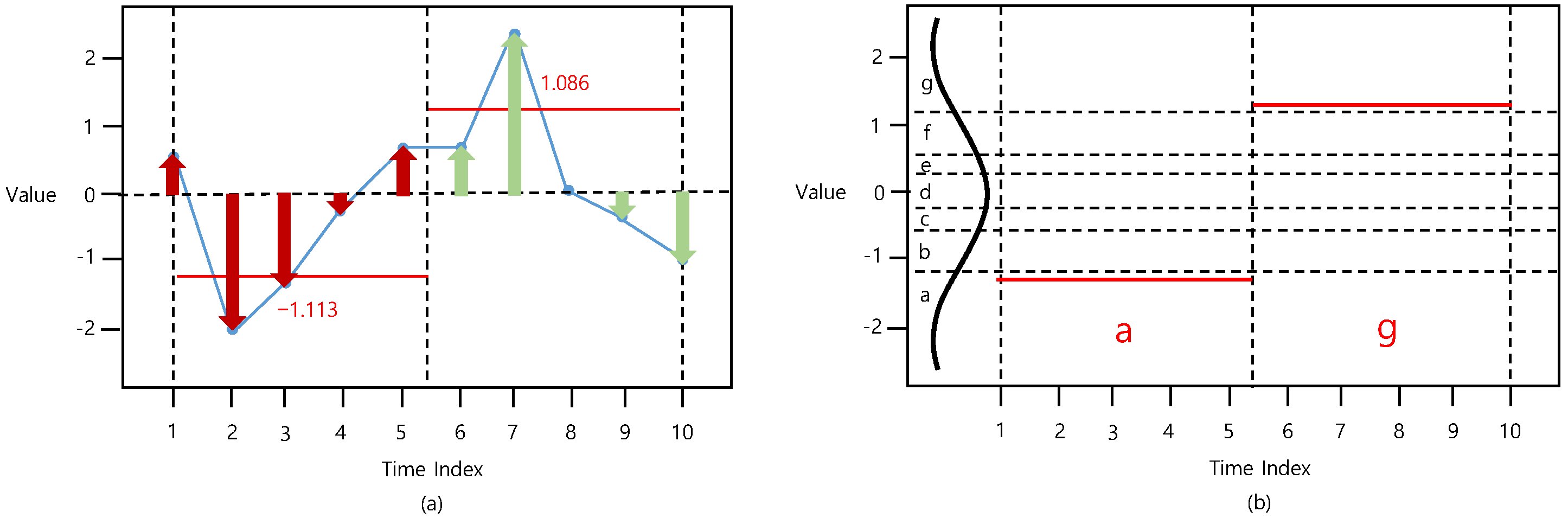
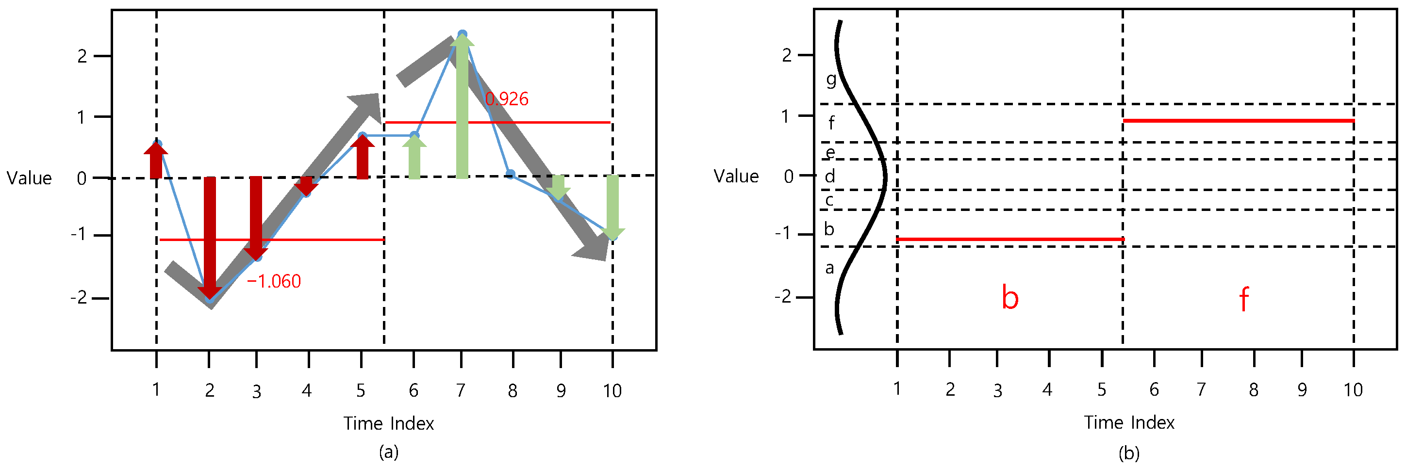
3.2. DM-SAX
4. Experimental Validation
4.1. UCR Datasets
4.1.1. Experimental Design
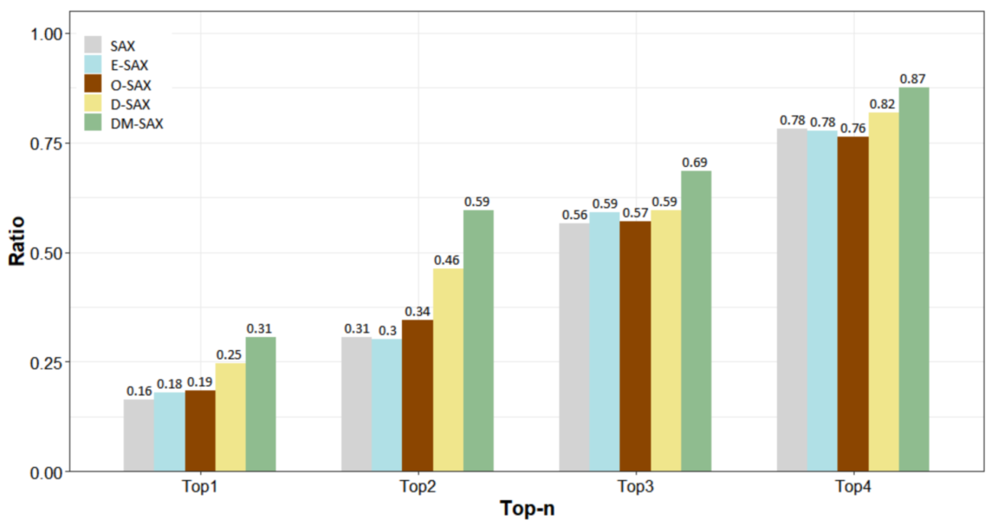
4.1.2. Experimental Results
4.2. Real-World Manufacturing Process Dataset
4.2.1. Experimental Design
4.2.2. Experimental Results
5. Conclusions
Author Contributions
Funding
Institutional Review Board Statement
Informed Consent Statement
Data Availability Statement
Conflicts of Interest
References
- Åström, K.J. On the Choice of Sampling Rates in Parametric Identification of Time Series. Inf. Sci. 1969, 1, 273–278. [Google Scholar] [CrossRef] [Green Version]
- Keogh, E.J.; Pazzani, M.J. A Simple Dimensionality Reduction Technique for Fast Similarity Search in Large Time Series Databases. In Lecture Notes in Computer Science, Proceedings of the 4th Pacific-Asia Conference on Knowledge Discovery and Data Mining, Kyoto, Japan, 18–20 April 2000; Springer: Berlin/Heidelberg, Germany, 2000; pp. 122–133. [Google Scholar] [CrossRef] [Green Version]
- Keogh, E.; Chakrabarti, K.; Pazzani, M.; Mehrotra, S. Locally Adaptive Dimensionality Reduction for Indexing Large Time Series Databases. In SIGMOD Rec, Proceedings of the 2001 ACM SIGMOD International Conference on Management of Data, Santa Barbara, CA, USA, 21–24 May 2001; Association for Computing Machinery: New York, NY, USA, 2001; Volume 30, pp. 151–162. [Google Scholar] [CrossRef] [Green Version]
- Guo, C.; Li, H.; Pan, D. An Improved Piecewise Aggregate Approximation Based on Statistical Features for Time Series Mining. In Lecture Notes in Computer Science, Proceedings of the International Conference on Knowledge Science, Engineering and Management, Belfast, UK, 1–3 September 2010; Springer: Berlin/Heidelberg, Germany, 2010; pp. 234–244. [Google Scholar] [CrossRef]
- Ren, H.; Liao, X.; Li, Z.; Ai-Ahmari, A. Anomaly Detection Using Piecewise Aggregate Approximation in the Amplitude Domain. Appl. Intell. 2018, 48, 1097–1110. [Google Scholar] [CrossRef]
- Dan, J.; Shi, W.; Dong, F.; Hirota, K. Piecewise trend approximation: A ratio-based time series representation. In Abstract and Applied Analysis; Hindawi Publishing: London, UK, 2013; Volume 2013. [Google Scholar]
- Yang, Z.; Zhao, G. Application of Symbolic Techniques in Detecting Determinism in Time Series. In Proceedings of the 20th Annual International Conference of the IEEE Engineering in Medicine and Biology Society, Hong Kong, China, 1 November 1998; Volume 20, pp. 2670–2673. [Google Scholar]
- Yang, O.; Jia, W.; Zhou, P.; Meng, X. A New Approach to Transforming Time Series into Symbolic Sequences. In Proceedings of the First Joint Conference Between the Biomedical Engineering Society and Engineers in Medicine and Biology, Atlanta, GA, USA, 13–16 October 1999; p. 974. [Google Scholar]
- Motoyoshi, M.; Miura, T.; Watanabe, K. Mining Temporal Classes from Time Series Data. In Proceedings of the 11th ACM International Conference on Information and Knowledge Management, McLean, VA, USA, 4–9 November 2002; pp. 493–498. [Google Scholar]
- Aref, W.G.; Elfeky, M.G.; Elmagarmid, A.K. Incremental, Online, and Merge Mining of Partial Periodic Patterns in Time-Series Databases. IEEE Trans. Knowl. Data Eng. 2004, 16, 335–345. [Google Scholar] [CrossRef] [Green Version]
- Lin, J.; Keogh, E.; Wei, L.; Lonardi, S. Experiencing SAX: A Novel Symbolic Representation of Time Series. Data Min. Knowl. Disc. 2007, 15, 107–144. [Google Scholar] [CrossRef] [Green Version]
- Zhao, X.; Shang, P.; Huang, J. Mutual-Information Matrix Analysis for Nonlinear Interactions of Multivariate Time Series. Nonlinear Dyn. 2017, 88, 477–487. [Google Scholar] [CrossRef]
- Park, H.; Jung, J.Y. SAX-ARM: Deviant Event Pattern Discovery from Multivariate Time Series Using Symbolic Aggregate Approximation and Association Rule Mining. Expert Syst. Appl. 2020, 141, 112950. [Google Scholar] [CrossRef]
- Ferreira, A.A.; Barbosa, I.; Rameh, M.B.; Aquino, R.R.; Manuel, H.; Natarajan, S.; Coley, D. Adaptive Piecewise and Symbolic Aggregate Approximation as an Improved Representation Method for Heat Waves Detection. In Science and Information Conference; Springer: Cham, Switzerland, 2018; pp. 658–671. [Google Scholar]
- Wu, H.W.; Lee, A.J. Mining Closed Flexible Patterns in Time-Series Databases. Expert Syst. Appl. 2010, 37, 2098–2107. [Google Scholar] [CrossRef]
- Ohsaki, M.; Sato, Y.; Yokoi, H.; Yamaguchi, T. A Rule Discovery Support System for Sequential Medical Data, in the Case Study of a Chronic Hepatitis Dataset. In Workshop Notes of the International Workshop on Active Mining, Proceedings of the IEEE International Conference on Data Mining; 2002; p. 121. Available online: https://scholar.google.com/scholar?hl=ko&as_sdt=0%2C5&q=A+Rule+Discovery+Support+System+for+Sequential+Medical+Data%2C+in+the+Case+Study+of+a+Chronic+Hepatitis+Dataset&btnG= (accessed on 30 May 2022).
- Tseng, V.S.; Chen, L.C.; Liu, J.J. Gene Relation Discovery by Mining Similar Subsequences in Time-Series Microarray Data. In IEEE Symposium on Computational Intelligence and Bioinformatics and Computational Biology; IEEE Publications: Piscataway, NJ, USA, 2007; Volume 2007, pp. 106–112. [Google Scholar]
- Ordóñez, P.; DesJardins, M.; Feltes, C.; Lehmann, C.U.; Fackler, J. Visualizing Multivariate Time Series Data to Detect Specific Medical Conditions. In AMIA Annual Symposium Proceedings; American Medical Informatics Association: Bethesda, MD, USA, 2008; Volume 2008. [Google Scholar]
- Yaik, O.B.; Yong, C.H.; Haron, F. CPU Usage Pattern Discovery Using Suffix Tree. In Proceedings of the 2nd International Conference on Distributed Frameworks for Multimedia Applications, Penang, Malaysia, 15–17 May 2006; IEEE Publications: Piscataway, NJ, USA, 2006; pp. 1–8. [Google Scholar]
- Pouget, F.; Urvoy-Keller, G.; Dacier, M. Time Signatures to Detect Multi-headed Stealthy Attack Tools. In Proceedings of the 18th Annual First Conference, Baltimore, MD, USA, 25–30 June 2006; Baltimore, M.D., Ed.; pp. 25–30. Available online: https://scholar.google.com/scholar?hl=ko&as_sdt=0%2C5&q=Time+Signatures+to+Detect+Multi-headed+Stealthy+Attack+Tools&btnG=#d=gs_cit&t=1657109401025&u=%2Fscholar%3Fq%3Dinfo%3A1whwFcShTrgJ%3Ascholar.google.com%2F%26output%3Dcite%26scirp%3D0%26hl%3Dko (accessed on 30 May 2022).
- Zoumboulakis, M.; Roussos, G. Escalation: Complex Event Detection in Wireless Sensor Networks. In Lecture Notes in Computer Science, Proceedings of the European Conference on Smart Sensing and Context, Kendal, UK, 23–25 October 2007; Springer: Berlin/Heidelberg, Germany, 2007; pp. 270–285. [Google Scholar] [CrossRef] [Green Version]
- McGovern, A.; Rosendahl, D.H.; Brown, R.A. Toward Understanding Tornado Formation Through Spatiotemporal Data Mining. In Data Mining for Geoinformatics; Springer: New York, NY, USA, 2014; pp. 29–47. [Google Scholar]
- Ciompi, F.; Pujol, O.; Balocco, S.; Carrillo, X.; Mauri-Ferré, J.; Radeva, P. Automatic Key Frames Detection in Intravascular Ultrasound Sequences. In Proceedings of the 14th Medical Image Computing and Computer Assisted Intervention Society, Toronto, ON, Canada, 18–22 September 2011; pp. 78–94. [Google Scholar]
- Shie, B.E.; Jang, F.L.; Tseng, V.S. Intelligent Panic Disorder Treatment by Using Biofeedback Analysis and Web Technologies. Int. J. Bus. Intell. Data Min. 2010, 5, 77–93. [Google Scholar] [CrossRef]
- Morgan, I.; Liu, H.; Turnbull, G.; Brown, D. Time Discretisation Applied to Anomaly Detection in a Marine Engine. In Proceedings of the International Conference on Knowledge-Based and Intelligent Information and Engineering Systems, Vietri sul Mare, Italy, 12–14 September 2007; Springer: Berlin/Heidelberg, Germany, 2007; pp. 405–412. [Google Scholar]
- He, W.; Xiang, H.; Tang, J. Analog-Circuit Fault Diagnosis Using Three-Stage Preprocessing and Time Series Data Mining. In Proceedings of the IEEE Circuits and Systems International Conference on Testing and Diagnosis, Chengdu, China, 28–29 April 2009; IEEE Publications: Piscataway, NJ, USA, 2009; Volume 2009, pp. 1–4. [Google Scholar]
- Fuad, M.; Marwan, M. Extreme-SAX: Extreme Points Based Symbolic Representation for Time Series Classification. In Proceedings of the International Conference on Big Data Analytics and Knowledge Discovery, Bratislava, Slovakia, 14–17 September 2020; Springer: Cham, Switzerland, 2020; pp. 122–130. [Google Scholar]
- Lkhagva, B.; Suzuki, Y.; Kawagoe, K. Extended SAX: Extension of Symbolic Aggregate Approximation for Financial Time Series Data Representation. DEWS2006 4A-i8, 7. Available online: https://www.ieice.org/~de/DEWS/DEWS2006/doc/4A-i8.pdf (accessed on 30 May 2022).
- Lin, J.; Li, Y. Finding Structural Similarity in Time Series Data Using Bag-of-Patterns Representation. In Lecture Notes in Computer Science, Proceedings of the International Conference on Scientific and Statistical Database Management, New Orleans, LA, USA, 2–4 June 2009; Springer: Berlin/Heidelberg, Germany, 2009; pp. 461–477. [Google Scholar] [CrossRef]
- Senin, P.; Malinchik, S. Sax-Vsm: Interpretable Time Series Classification Using Sax and Vector Space Model. In Proceedings of the 13th International Conference on Data Mining, Dallas, TX, USA, 7–10 December 2013; IEEE Publications: Piscataway, NJ, USA, 2013; Volume 2013, pp. 1175–1180. [Google Scholar]
- Fuad, M.; Marwan, M. Modifying the Symbolic Aggregate Approximation Method to Capture Segment Trend Information. In Proceedings of the International Conference on Modeling Decisions for Artificial Intelligence, Sant Cugat, Spain, 2–4 September 2020; Springer: Cham, Switzerland, 2020; pp. 230–239. [Google Scholar]
- Song, K.; Ryu, M.; Lee, K. Transitional Sax Representation for Knowledge Discovery for Time Series. Appl. Sci. 2020, 10, 6980. [Google Scholar] [CrossRef]
- Sun, Y.; Li, J.; Liu, J.; Sun, B.; Chow, C. An Improvement of Symbolic Aggregate Approximation Distance Measure for Time Series. Neurocomputing 2014, 138, 189–198. [Google Scholar] [CrossRef]
- Yin, H.; Yang, S.Q.; Zhu, X.Q.; Ma, S.D.; Zhang, L.M. Symbolic Representation Based on Trend Features for Knowledge Discovery in Long Time Series. Front. Inf. Technol. Electron. Eng. 2015, 16, 744–758. [Google Scholar] [CrossRef]
- Malinowski, S.; Guyet, T.; Quiniou, R.; Tavenard, R. 1d-Sax: A Novel Symbolic Representation for Time Series. In Lecture Notes in Computer Science, Proceedings of the International Symposium on Intelligent Data Analysis, London, UK, 17–19 October 2013; Springer: Berlin/Heidelberg, Germany, 2013; pp. 273–284. [Google Scholar] [CrossRef] [Green Version]
- Fuad, M.; Marwan, M. Genetic Algorithms-Based Symbolic Aggregate Approximation. In Proceedings of the International Conference on Data Warehousing and Knowledge Discovery, Vienna, Austria, 3–6 September 2012; Springer: Berlin/Heidelberg, Germany, 2012; pp. 105–116. [Google Scholar]
- Allani, S. SAX-BOP: Epileptic Seizure Detection Using Symbolic Aggregate Approximation and Bag of Patterns. Master’s Thesis, University of Maryland, Baltimore County, MD, USA, 2014. [Google Scholar]
- Aremu, O.O.; Hyland-Wood, D.; McAree, P.R. A Relative Entropy Weibull-Sax Framework for Health Indices Construction and Health Stage Division in Degradation Modeling of Multivariate Time Series Asset Data. Adv. Eng. Inform. 2019, 40, 121–134. [Google Scholar] [CrossRef]
- Kamath, U.; Lin, J.; De Jong, K. SAX-EFG: An Evolutionary Feature Generation Framework for Time Series Classification. In Proceedings of the 2014 Annual Conference on Genetic and Evolutionary Computation, Vancouver, BC, Canada, 12–16 July 2014; pp. 533–540. [Google Scholar]
- Mekami, H.; Benabderrahmane, S. SAX2FACE: Estimating Facial Poses with Peano-Hilbert Curves and Sax Symbolic Time Series. Procedia Comput. Sci. 2017, 109, 217–224. [Google Scholar] [CrossRef]
- Zan, C.T.; Yamana, H. An Improved Symbolic Aggregate Approximation Distance Measure Based on its Statistical Features. In Proceedings of the 18th International Conference on Information Integration and Web-Based Applications and Services, Singapore, 28–30 November 2016; pp. 72–80. [Google Scholar]
- Geng, Y.; Luo, X. Cost-Sensitive Convolution Based Neural Networks for Imbalanced Time-Series Classification. arXiv 2018, arXiv:1801.04396. [Google Scholar]
- Duque-Pintor, F.J.; Fernández-Gómez, M.J.; Troncoso, A.; Martínez-Álvarez, F. A New Methodology Based on Imbalanced Classification for Predicting Outliers in Electricity Demand Time Series. Energies 2016, 9, 752. [Google Scholar] [CrossRef] [Green Version]
- Troncoso, A.; Ribera, P.; Asencio-Cortés, G.; Vega, I.; Gallego, D. Imbalanced Classification Techniques for Monsoon Forecasting Based on a New Climatic Time Series. Environ. Modell. Softw. 2018, 106, 48–56. [Google Scholar] [CrossRef]
- He, H.; Garcia, E.A. Learning from imbalanced data. IEEE Trans. Knowl. Data Eng. 2009, 21, 1263–1284. [Google Scholar] [CrossRef]
- Dau, H.A.; Bagnall, A.; Kamgar, K.; Yeh, C.M.; Zhu, Y.; Gharghabi, S.; Ratanamahatana, C.A.; Keogh, E.; Keogh, E. The UCR Time Series Archive. IEEE CAA J. Autom. Sin. 2019, 6, 1293–1305. [Google Scholar] [CrossRef]
- Breiman, L. Random Forests. Mach. Learn. 2001, 45, 5–32. [Google Scholar] [CrossRef] [Green Version]
- Oshiro, T.M.; Perez, P.S.; Baranauskas, J.A. How Many Trees in a Random Forest? In Lecture Notes in Computer Science, Proceedings of the International Workshop on Machine Learning and Data Mining in Pattern Recognition, Berlin, Germany, 13–20 July 2012; Springer: Berlin/Heidelberg, Germany, 2012; pp. 154–168. [Google Scholar] [CrossRef]
- Biau, G.; Scornet, E. A Random Forest Guided Tour. Test 2016, 25, 197–227. [Google Scholar] [CrossRef] [Green Version]
- Svetnik, V.; Liaw, A.; Tong, C.; Culberson, J.C.; Sheridan, R.P.; Feuston, B.P. Random Forest: A Classification and Regression Tool for Compound Classification and QSAR Modeling. J. Chem. Inf. Comput. Sci. 2003, 43, 1947–1958. [Google Scholar] [CrossRef] [PubMed]
- Cao, P.; Zhao, D.; Zaiane, O. An Optimized Cost-Sensitive SVM for Imbalanced Data Learning. In Lecture Notes in Computer Science, Proceedings of the Pacific-Asia Conference on Knowledge Discovery and Data Mining, Gold Coast, Australia, 14–17 April 2013; Springer: Berlin/Heidelberg, Germany, 2013; pp. 280–292. [Google Scholar] [CrossRef] [Green Version]
- Akosa, J. Predictive Accuracy: A Misleading Performance Measure for Highly Imbalanced Data. In Proceedings of the SAS Global Forum; 2017; Volume 12, Available online: https://support.sas.com/resources/papers/proceedings17/0942-2017.pdf (accessed on 30 May 2022).
- Demšar, J. Statistical Comparisons of Classifiers over Multiple Data Sets. J. Mach. Learn. Res. 2006, 7, 1–30. [Google Scholar]
- Benavoli, A.; Corani, G.; Mangili, F. Should We Really Use Post-hoc Tests Based on Mean-Ranks? J. Mach. Learn. Res. 2016, 17, 152–161. [Google Scholar]
- Armstrong, R.A. When to Use the Bonferroni Correction. Ophthalmic Physiol. Opt. 2014, 34, 502–508. [Google Scholar] [CrossRef] [PubMed]


| n_bins | 3 | 4 | 5 | 6 | 7 | 8 | 9 | 10 | |
|---|---|---|---|---|---|---|---|---|---|
| βi | |||||||||
| −0.43 | −0.67 | −0.84 | −0.97 | −1.07 | −1.15 | −1.22 | −1.28 | ||
| 0.43 | 0.00 | −0.25 | −0.43 | −0.57 | −0.67 | −0.76 | −0.84 | ||
| 0.67 | 0.25 | 0.00 | −0.18 | −0.32 | −0.43 | −0.52 | |||
| 0.84 | 0.43 | 0.18 | 0.00 | −0.14 | −0.25 | ||||
| 0.97 | 0.57 | 0.32 | 0.14 | −0.00 | |||||
| 1.07 | 0.67 | 0.43 | 0.25 | ||||||
| 1.15 | 0.76 | 0.52 | |||||||
| 1.22 | 0.84 | ||||||||
| 1.28 | |||||||||
| Dataset | #Training Data Points | #Test Data Points | #Input Features | Imbalance Ratio |
|---|---|---|---|---|
| Adiac | 390 | 391 | 176 | 38.1 |
| CricketX | 390 | 390 | 300 | 11.0 |
| CricketY | 390 | 390 | 300 | 11.0 |
| CricketZ | 390 | 390 | 300 | 11.0 |
| Crop | 7200 | 16,800 | 46 | 23.0 |
| DistalPhalanxOutlineAgeGroup | 400 | 139 | 80 | 11.0 |
| DistalPhalanxTW | 400 | 139 | 80 | 19.7 |
| ECG5000 | 500 | 5000 | 140 | 207.3 |
| ElectricDevices | 8926 | 7711 | 96 | 12.3 |
| EOGHorizontalSignal | 362 | 362 | 1250 | 11.3 |
| EOGVerticalSignal | 362 | 362 | 1250 | 11.3 |
| FaceAll | 560 | 1690 | 131 | 45.9 |
| FacesUCR | 200 | 2050 | 131 | 45.9 |
| FiftyWords | 450 | 455 | 270 | 149.8 |
| Fungi | 18 | 186 | 201 | 24.5 |
| InsectWingbeatSound | 220 | 1980 | 256 | 10.0 |
| MedicalImages | 381 | 760 | 99 | 48.6 |
| MiddlePhalanxTW | 399 | 154 | 80 | 15.3 |
| NonInvasiveFetalECGThorax1 | 1800 | 1965 | 750 | 49.2 |
| NonInvasiveFetalECGThorax2 | 1800 | 1965 | 750 | 49.2 |
| OSULeaf | 200 | 242 | 427 | 10.6 |
| Phoneme | 214 | 1896 | 1024 | 1054.0 |
| PigAirwayPressure | 104 | 208 | 2000 | 51.0 |
| PigArtPressure | 104 | 208 | 2000 | 51.0 |
| PigCVP | 104 | 208 | 2000 | 51.0 |
| ProximalPhalanxTW | 400 | 205 | 80 | 32.6 |
| ShapesAll | 600 | 600 | 512 | 59.0 |
| SwedishLeaf | 500 | 625 | 128 | 14.0 |
| WordSynonyms | 267 | 638 | 270 | 74.4 |
| Dataset | SAX | E-SAX | O-SAX | D-SAX | DM-SAX |
|---|---|---|---|---|---|
| Adiac | 43.10 | 52.64 | 50.01 | 48.34 | 48.97 |
| CricketX | 55.78 | 58.68 | 60.93 | 61.01 | 60.23 |
| CricketY | 68.84 | 71.62 | 63.95 | 72.73 | 72.54 |
| CricketZ | 51.33 | 52.90 | 51.57 | 52.42 | 52.86 |
| Crop | 99.55 | 99.42 | 99.73 | 99.64 | 99.64 |
| DistalPhalanxOutlineAgeGroup | 89.31 | 93.06 | 83.92 | 82.48 | 81.54 |
| DistalPhalanxTW | 50.73 | 54.51 | 57.16 | 56.74 | 57.51 |
| ECG5000 | 65.72 | 58.09 | 60.87 | 66.54 | 67.04 |
| ElectricDevices | 80.55 | 78.34 | 80.56 | 84.80 | 84.02 |
| EOGHorizontalSignal | 72.34 | 76.00 | 77.95 | 73.75 | 74.37 |
| EOGVerticalSignal | 69.57 | 70.84 | 76.62 | 69.94 | 69.14 |
| FaceAll | 94.29 | 92.89 | 89.28 | 96.09 | 97.15 |
| FacesUCR | 61.33 | 55.96 | 59.05 | 65.01 | 63.88 |
| FiftyWords | 60.54 | 65.93 | 58.70 | 60.86 | 61.54 |
| Fungi | 98.12 | 86.14 | 93.89 | 97.77 | 97.89 |
| InsectWingbeatSound | 76.53 | 62.60 | 71.30 | 78.31 | 78.83 |
| MedicalImages | 77.95 | 87.85 | 90.21 | 95.24 | 95.75 |
| MiddlePhalanxTW | 63.70 | 69.12 | 68.31 | 66.15 | 71.17 |
| NonInvasiveFetalECGThorax1 | 85.80 | 87.12 | 67.86 | 92.76 | 92.31 |
| NonInvasiveFetalECGThorax2 | 82.04 | 81.11 | 67.12 | 87.23 | 87.72 |
| OSULeaf | 57.59 | 47.28 | 56.51 | 57.78 | 58.30 |
| Phoneme | 36.33 | 69.76 | 69.82 | 53.56 | 53.52 |
| PigAirwayPressure | 59.11 | 81.37 | 84.45 | 64.83 | 66.59 |
| PigArtPressure | 60.70 | 51.64 | 39.82 | 76.63 | 77.15 |
| PigCVP | 73.18 | 47.11 | 60.54 | 86.58 | 84.24 |
| ProximalPhalanxTW | 56.00 | 72.25 | 55.87 | 71.74 | 74.06 |
| ShapesAll | 82.38 | 74.49 | 89.97 | 85.76 | 84.61 |
| SwedishLeaf | 64.70 | 72.39 | 59.80 | 65.72 | 63.80 |
| WordSynonyms | 51.43 | 57.13 | 57.09 | 54.18 | 53.32 |
| Mean AUC (%) | 68.57 | 69.94 | 69.06 | 73.26 | 73.44 |
| Mean Rank | 3.86 | 3.21 | 3.24 | 2.41 | 2.24 |
| SAX | E-SAX | O-SAX | D-SAX | DM-SAX | |
|---|---|---|---|---|---|
| SAX | - | 0.9573 | 0.6517 | 0.0135 | 0.0022 |
| E-SAX | - | 0.9222 | 0.0139 | 0.0032 | |
| O-SAX | 0.0251 | 0.0043 | |||
| D-SAX | - | 0.2692 | |||
| DM-SAX | - |
| Features | Description |
|---|---|
| B/S | Bad limit overall/Specification delta conductor |
| RCFA | Results measured from crimp force analyzer |
| MPP | Maximum press power |
| Features | Min | Median | Mean | Max |
|---|---|---|---|---|
| B/S | −2052.0 | 1.0 | −1.1 | 1674.0 |
| RCFA | 1.0 | 14.0 | 17.4 | 2052.0 |
| MPP | 99.0 | 3457.0 | 3774.8 | 8758.0 |
| Elements | UCR | Real-World | |
|---|---|---|---|
| Similarities | Competing methods | SAX, E-SAX, O-SAX, D-SAX, and DM-SAX | |
| Performance measure | AUC | ||
| Base classifier | Random forest (20 iterations) | ||
| n_bins | 4, 6, 8, and 10 | ||
| a | 0.9 | ||
| 0.01 | |||
| Differences | t_size | 3, 5 | 25, 50, 75, 100, and 150 |
| Training/Test set ratio | Originally split in the archive | 0.7/0.3 | |
| t_size | n_bins | SAX | E-SAX | O-SAX | D-SAX | DM-SAX |
|---|---|---|---|---|---|---|
| 25 | 4 | 85.16 | 89.45 | 87.74 | 99.39 | 99.38 |
| 6 | 85.00 | 94.18 | 93.58 | 99.73 | 99.76 | |
| 8 | 80.30 | 93.95 | 93.69 | 99.88 | 99.88 | |
| 10 | 83.23 | 93.68 | 92.28 | 99.34 | 99.33 | |
| 50 | 4 | 85.90 | 81.48 | 86.89 | 98.95 | 98.95 |
| 6 | 82.32 | 89.86 | 89.51 | 99.02 | 99.02 | |
| 8 | 84.67 | 93.17 | 87.87 | 99.50 | 99.47 | |
| 10 | 84.72 | 93.39 | 90.14 | 99.52 | 99.52 | |
| 75 | 4 | 79.29 | 77.62 | 85.28 | 99.27 | 99.27 |
| 6 | 76.83 | 88.39 | 86.97 | 98.96 | 98.96 | |
| 8 | 78.56 | 91.91 | 86.79 | 98.57 | 98.57 | |
| 10 | 76.23 | 92.53 | 86.79 | 98.95 | 98.96 | |
| 100 | 4 | 84.58 | 76.34 | 85.81 | 98.39 | 98.40 |
| 6 | 81.79 | 89.40 | 86.52 | 98.55 | 98.56 | |
| 8 | 78.48 | 92.79 | 87.77 | 97.79 | 98.27 | |
| 10 | 76.17 | 93.57 | 86.44 | 98.44 | 98.91 | |
| 150 | 4 | 77.27 | 73.90 | 82.60 | 97.75 | 97.76 |
| 6 | 78.45 | 86.71 | 82.03 | 98.06 | 98.08 | |
| 8 | 82.87 | 91.48 | 80.41 | 98.62 | 98.66 | |
| 10 | 79.05 | 91.37 | 78.79 | 97.45 | 97.90 | |
| Mean AUC (%) | 81.04 | 88.76 | 86.90 | 98.81 | 98.88 | |
| Mean Rank | 4.70 | 3.40 | 3.90 | 1.50 | 1.15 |
Publisher’s Note: MDPI stays neutral with regard to jurisdictional claims in published maps and institutional affiliations. |
© 2022 by the authors. Licensee MDPI, Basel, Switzerland. This article is an open access article distributed under the terms and conditions of the Creative Commons Attribution (CC BY) license (https://creativecommons.org/licenses/by/4.0/).
Share and Cite
Yang, D.-H.; Kang, Y.-S. Distance- and Momentum-Based Symbolic Aggregate Approximation for Highly Imbalanced Classification. Sensors 2022, 22, 5095. https://doi.org/10.3390/s22145095
Yang D-H, Kang Y-S. Distance- and Momentum-Based Symbolic Aggregate Approximation for Highly Imbalanced Classification. Sensors. 2022; 22(14):5095. https://doi.org/10.3390/s22145095
Chicago/Turabian StyleYang, Dong-Hyuk, and Yong-Shin Kang. 2022. "Distance- and Momentum-Based Symbolic Aggregate Approximation for Highly Imbalanced Classification" Sensors 22, no. 14: 5095. https://doi.org/10.3390/s22145095