
Metal Surface Defect Detection Method Based on TE01 Mode Microwave


Abstract
:1. Introduction
2. Metal Surface Defect Identification Method
2.1. Transverse Wave (TEmn Wave) in Rectangular Waveguide
2.2. Microwave Detection Model of Metal Surface Defects
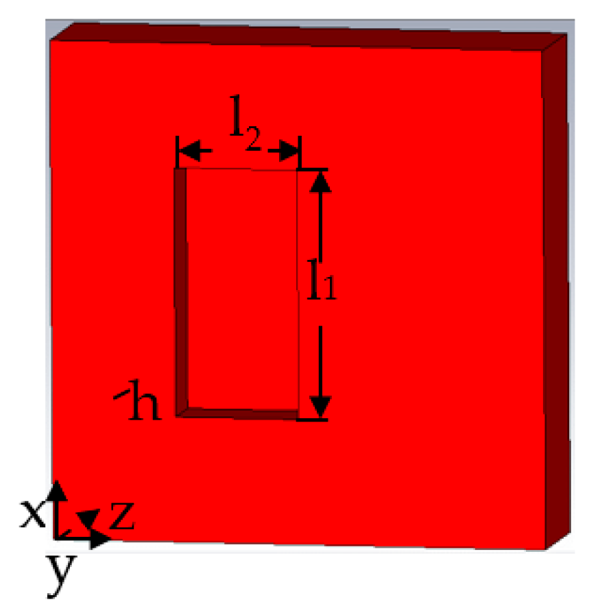
2.2.1. Metal Surface Defect Detection Model in Cartesian Coordinates
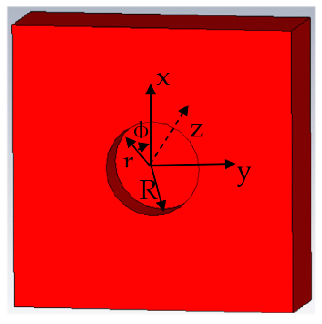
2.2.2. The Metal Surface Defect Detection Model under Cylindrical Coordinates
3. Simulation Model of Microwave Defect Detection in TE01 Mode
3.1. TE01-Mode Microwave Defect Detection Model
3.1.1. TE01-Mode Microwave Defect Detection Model at Crack Defects
3.1.2. TE01-Mode Microwave Defect Detection Model at Corrosion Defects
3.2. Microwave Detection Signal of TEO1 Mode Metal Surface Defect
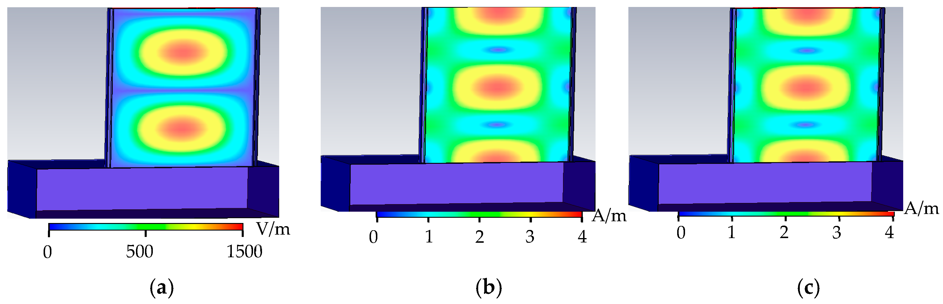
3.2.1. Rectangular Defect
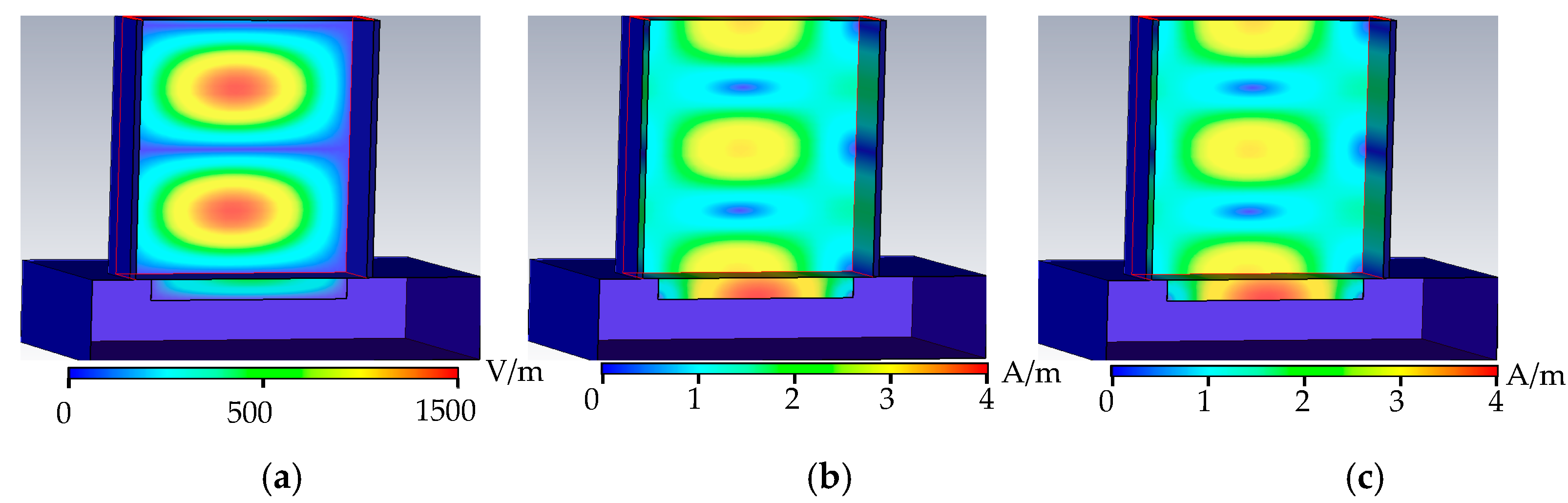
3.2.2. Cylindrical Defect
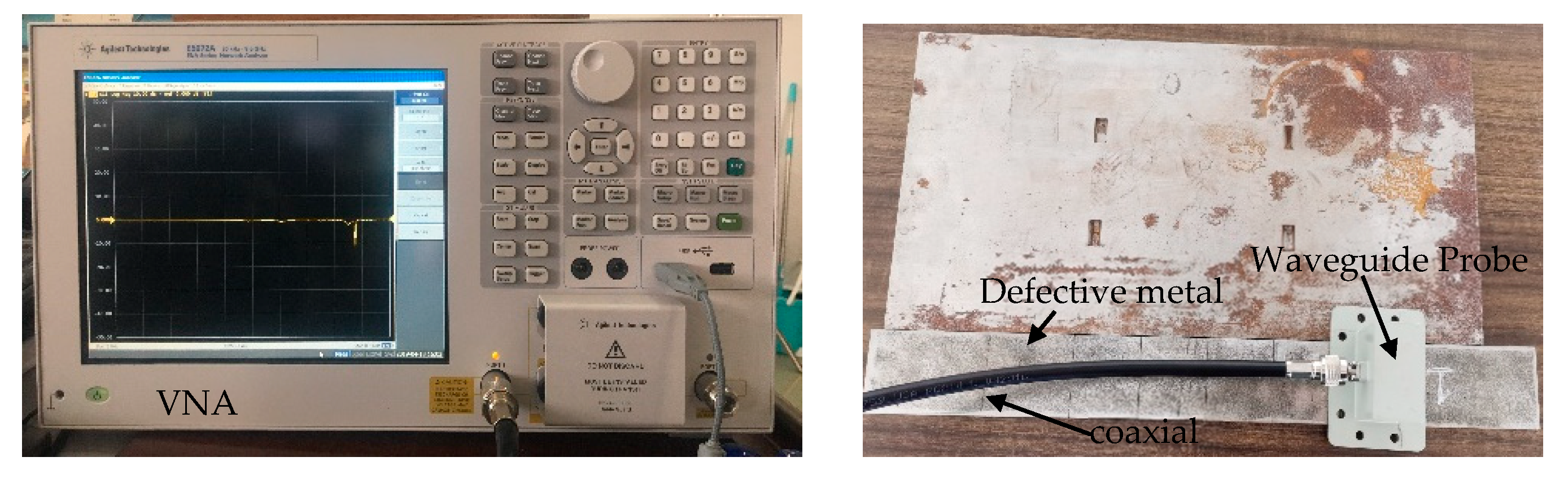
4. Experimental and Result Analysis
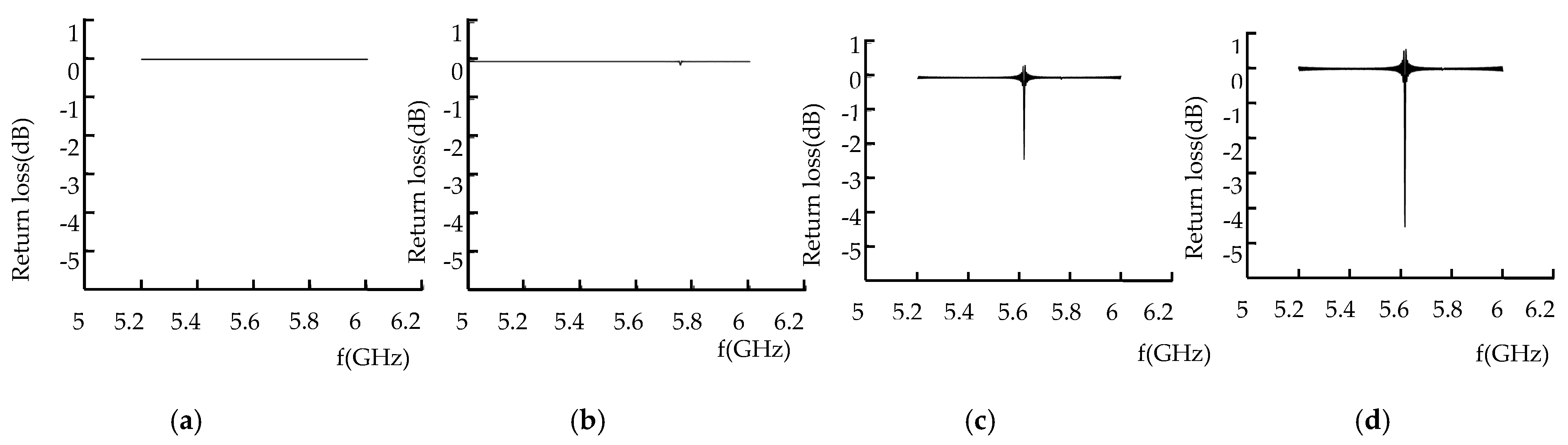
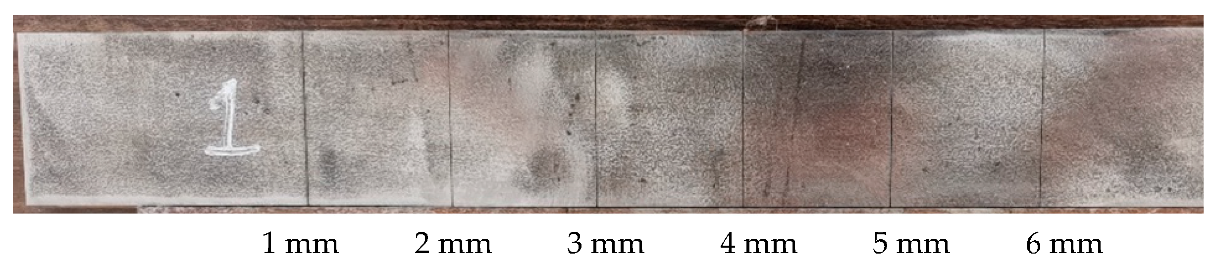
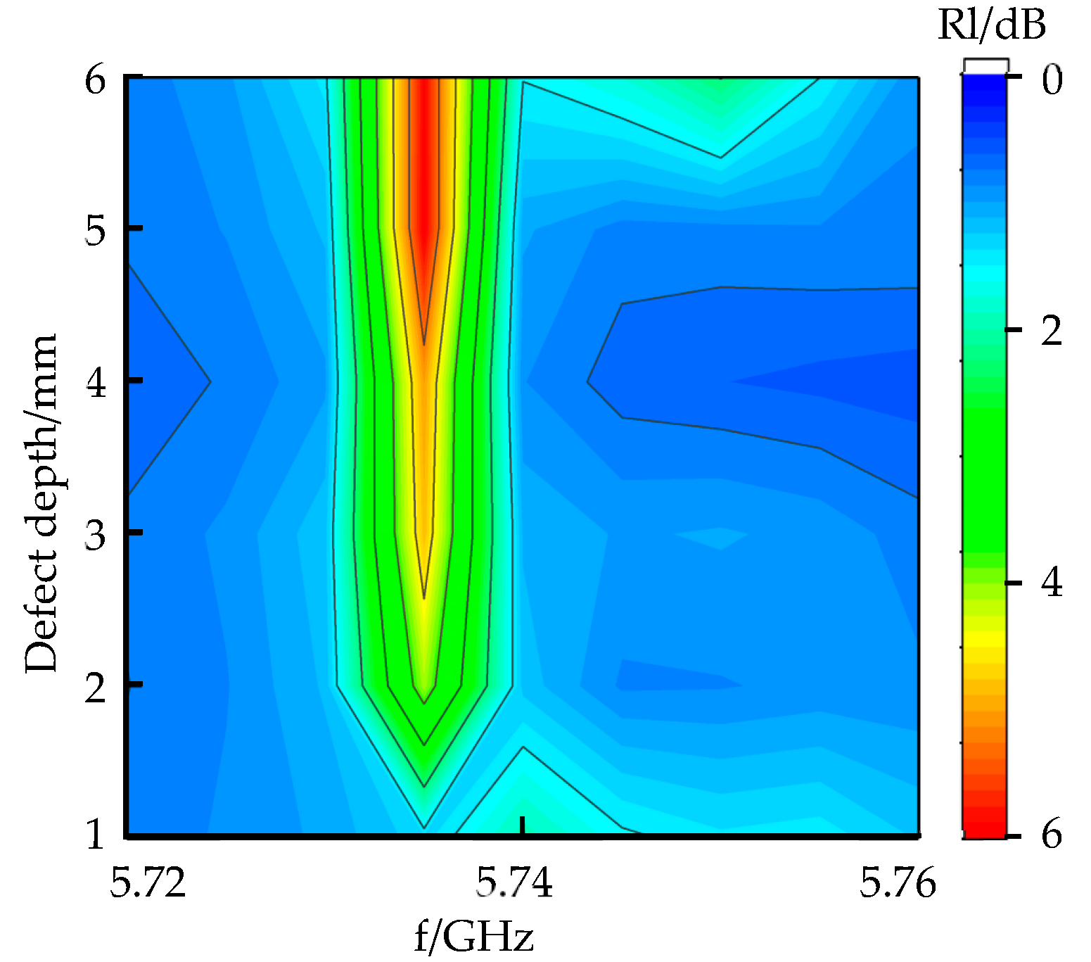
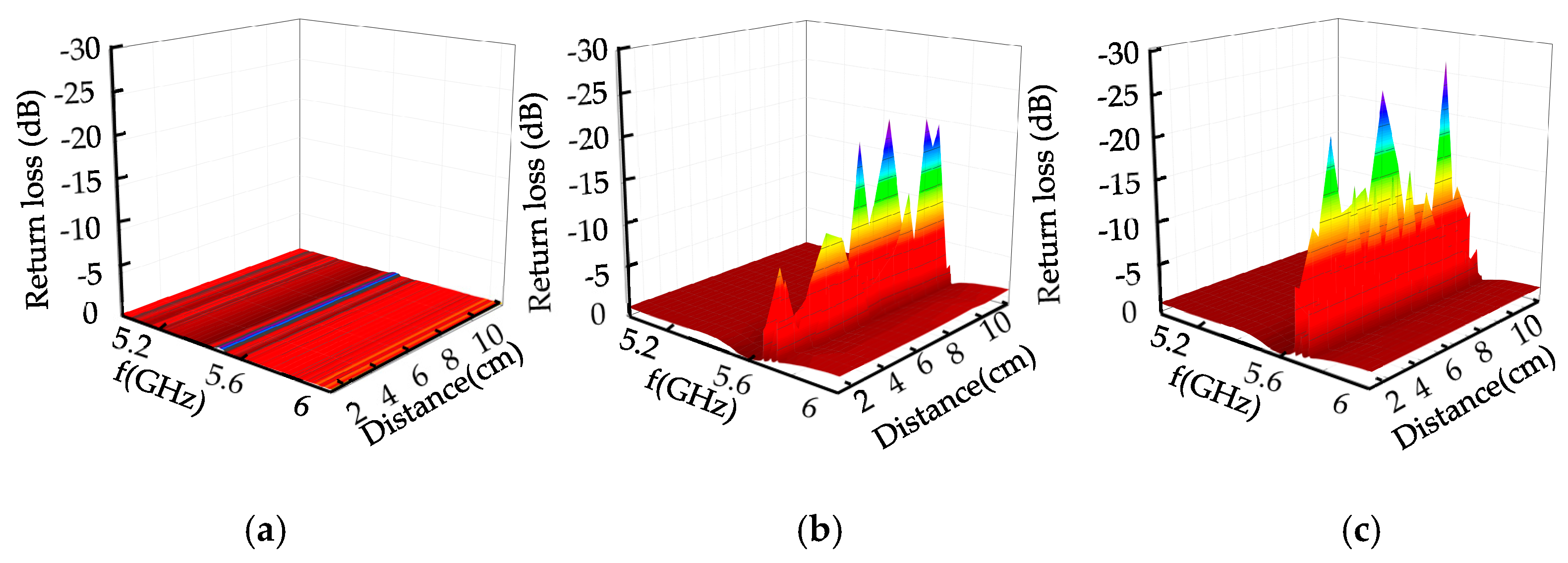
4.1. Microwave Inspection of TE01 Mode for Crack Defects with Different Depths
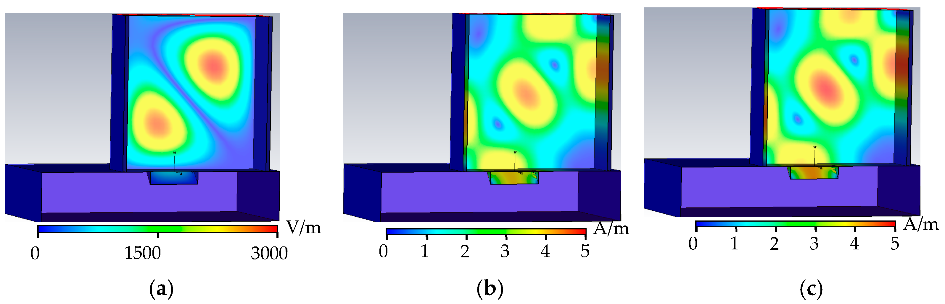
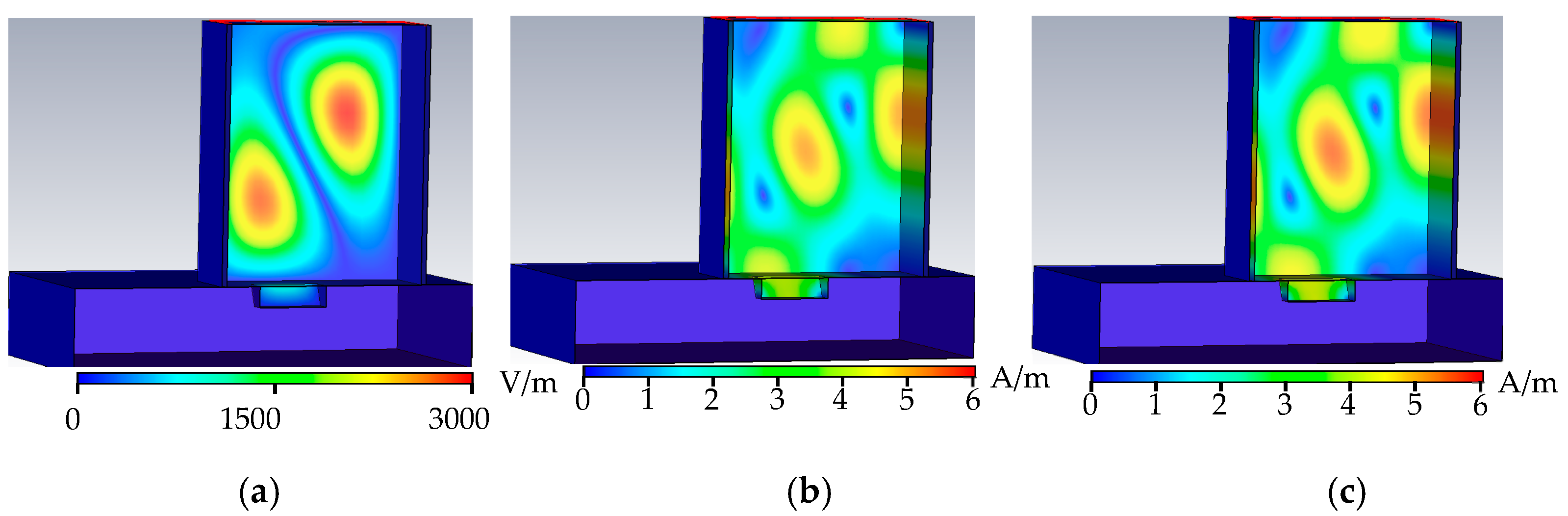
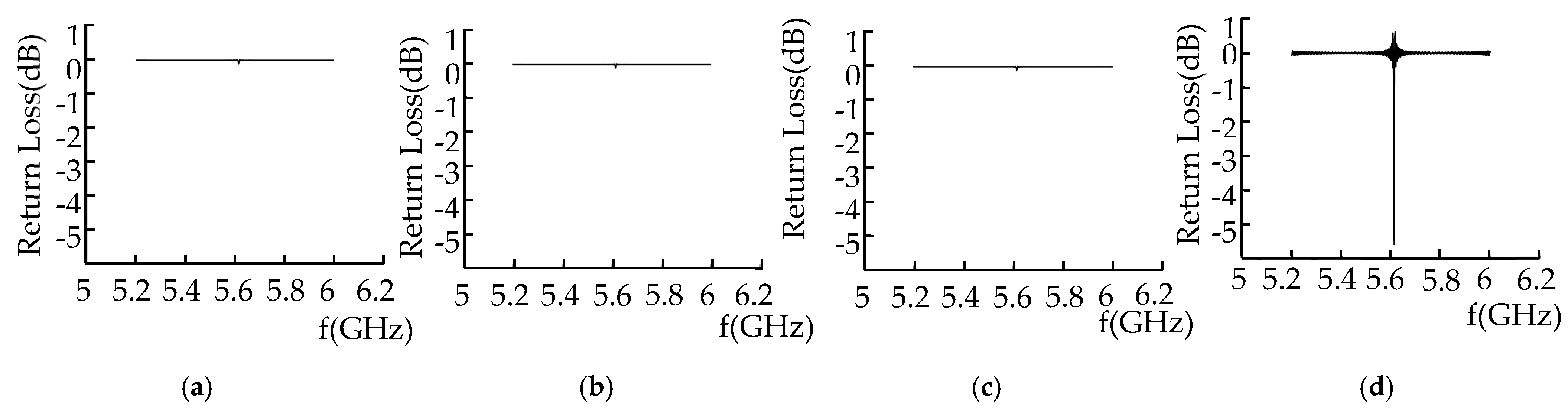
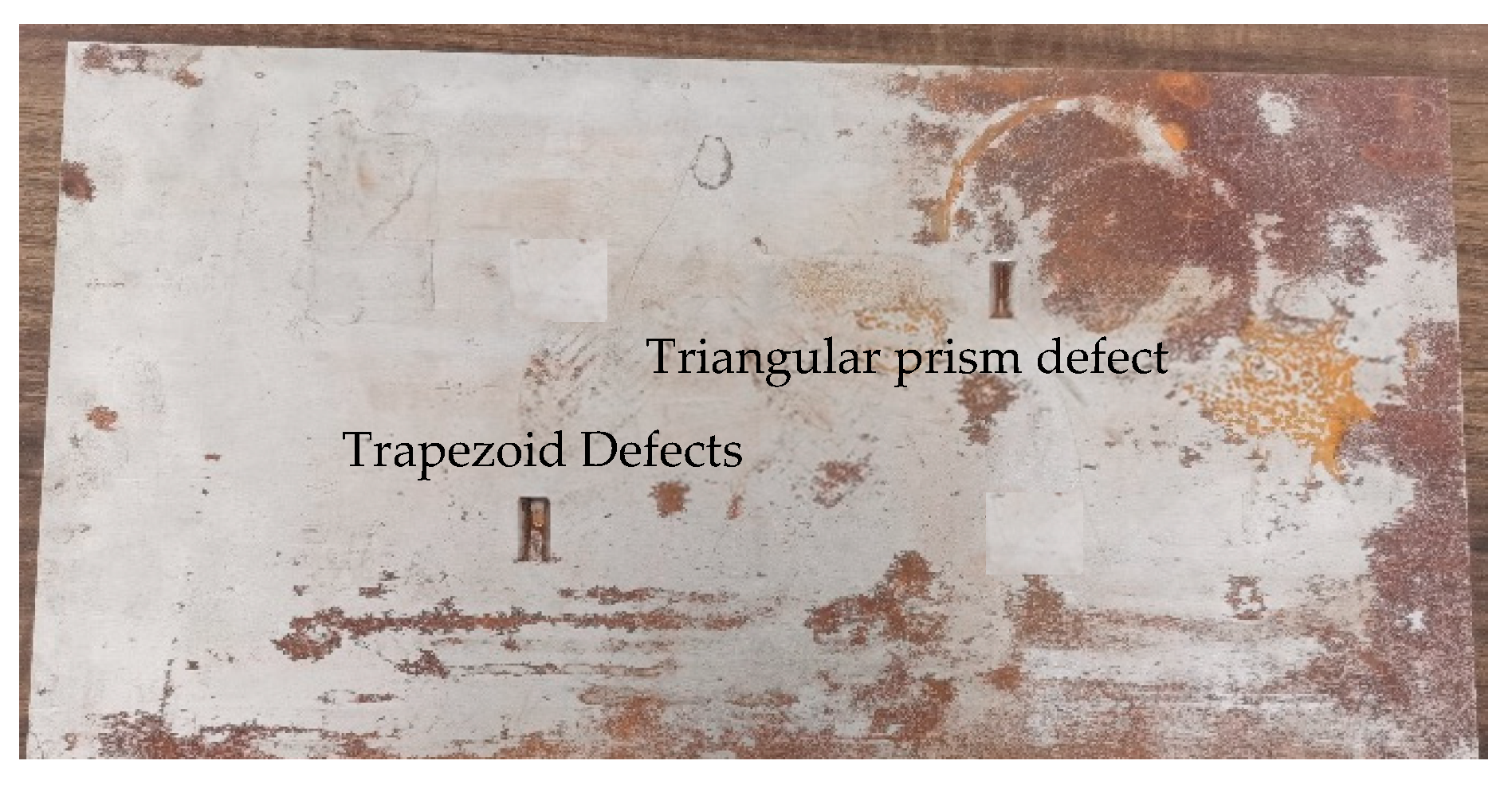
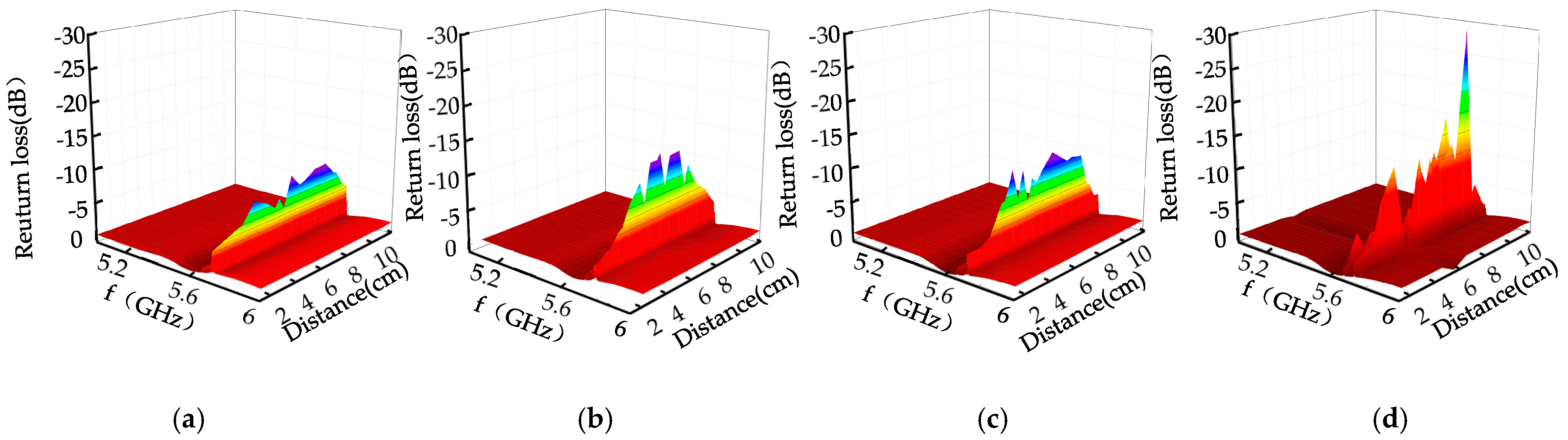
4.2. TE01-Mode Microwave Detection of Different Types of Rectangular Defects
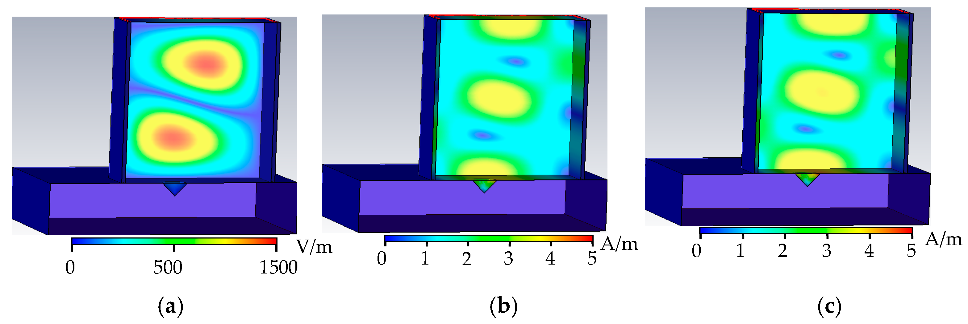
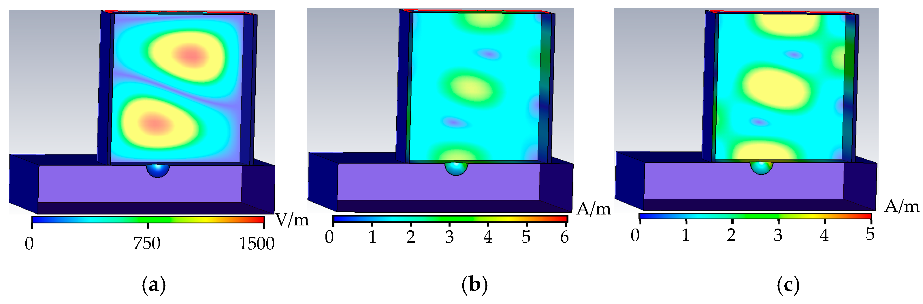
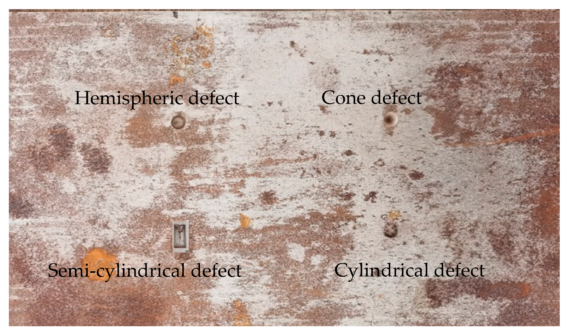
4.3. Detection of Cylindrical Defects of Different Sizes by TE01-Mode Microwave
5. Conclusions
- (1)
- In our study, we established a microwave detection model based on TE01-mode microwave in order to detect metal surface defects, established a relationship model between defect size and microwave reflection coefficient, and obtained a relationship model between microwave reflection coefficient and defect size;
- (2)
- Due to the existence of defects in the electric field, magnetic field, and tube wall current of the microwave propagation in the rectangular waveguide, the phase of the microwave propagation cycle is shifted, and the microwave energy is concentrated at the defect, resulting in energy loss and an increase in the return loss value.
- (3)
- The TE01-mode microwave can effectively detect 0.3 mm wide crack defects at 5.73 GHz, and the return loss value increases with the increase in defect depth; at 5.6 GHz, it can effectively detect 20 mm–wide trapezoid and triangular prism defects. The defect width increases, and the microwave detection frequency decreases; microwaves are more sensitive to crack defects with rectangular surfaces and more sensitive to defects with arc-shaped inner walls. The microwave has better detection ability for discontinuous surfaces.
Author Contributions
Funding
Institutional Review Board Statement
Informed Consent Statement
Data Availability Statement
Conflicts of Interest
References
- Yang, L.J.; Geng, H.; Gao, S.W. Magnetic flux leakage internal detection technology of the long distance oil pipeline. Chin. J. Sci. Instrum. 2016, 37, 1736–1746. [Google Scholar]
- Yang, L.J.; Liang, C.Z.; Gao, S.W. Analytical model of magnetic flux leakage field of pipe wall defects based on magnetic flux leakage internal detection. J. Electron. Meas. Instrum. 2021, 35, 106–114. [Google Scholar]
- Yang, L.J.; Zhang, X.D.; Gao, S.W. Research on the Propagation characteristics of ultrasonic wave in detection of pipeline coating. J. Electron. Meas. Instrum. 2018, 32, 9–18. [Google Scholar]
- Yang, L.J.; Xing, Y.H.; Zhang, J.; Gao, S. Crack defect detection of aluminum plate based on electromagnetic ultrasonic guided wave. Chin. J. Sci. Instrum. 2018, 39, 150–160. [Google Scholar]
- Olisa, S.; Khan, M.; Starr, A. Review of Current Guided Wave Ultrasonic Testing (GWUT) Limitations and Future Directions. Sensors 2021, 21, 811. [Google Scholar] [CrossRef]
- Zhang, N.; Peng, L.; Wu, Y. ECT probe based on magnetic field imaging with a high resolution TMR sensor array. Chin. J. Sci. Instrum. 2020, 41, 45–53. [Google Scholar]
- Li, W.; Duan, S.Y.; Song, Y. A pulse eddy current thickness measurement method of stainless steel plate based on Laplace wavelet’s characteristic frequency. Chin. J. Sci. Instrum. 2020, 41, 166–172. [Google Scholar]
- AbdAlla, A.N.; Faraj, M.A.; Samsuri, F.; Rifai, D.; Ali, K.; Al-Douri, Y. Challenges in improving the performance of eddy current testing: Review. Meas. Control. 2019, 52, 46–64. [Google Scholar] [CrossRef] [Green Version]
- Shaloo, M.; Schnall, M.; Klein, T.; Huber, N.; Reitinger, B. A Review of Non-Destructive Testing (NDT) Techniques for Defect Detection: Application to Fusion Welding and Future Wire Arc Additive Manufacturing Processes. Materials 2022, 15, 3697. [Google Scholar] [CrossRef]
- Geng, C.; Shi, W.; Liu, Z.; Xie, H.; He, W. Nondestructive Surface Crack Detection of Laser-Repaired Components by Laser Scanning Thermography. Appl. Sci. 2022, 12, 5665. [Google Scholar] [CrossRef]
- Arun, M.; Sumathi, P. Crack detection using image processing: A critical review and analysis. Alex. Eng. J. 2018, 57, 787–798. [Google Scholar]
- Müller, A.; Karathanasopoulos, N.; Roth, C.C.; Mohr, D. Machine Learning Classifiers for Surface Crack Detection in Fracture Experiments. Int. J. Mech. Sci. 2021, 209, 106698. [Google Scholar] [CrossRef]
- Wu, B.; He, L. Multilayered Circular Dielectric Structure SAR Imaging Based on Compressed Sensing for FOD Detection in NDT. IEEE Trans. Instrum. Meas. 2020, 29, 7588–7593. [Google Scholar] [CrossRef]
- Liu, L.; Yang, J.; Chen, M. Optimizing the frequency range of microwaves for high-resolution evaluation of wall thinning locations in a long-distance metal pipe. NDT E Int. 2013, 57, 52–57. [Google Scholar] [CrossRef]
- Lu, Y.; Liu, L.S.; Ishikawa, M. Quantitative Evaluation of Wall Thinning of Metal Pipes by Microwaves. Mater. Sci. Forum 2009, 614, 111–116. [Google Scholar] [CrossRef]
- Katagiri, T.; Sasaki, K.; Song, H.; Yusa, N.; Hashizume, H. Proposal of a TEM to TE01 mode converter for a microwave nondestructive inspection of axial flaws appearing on the inner surface of a pipe with an arbitrary diameter. Int. J. Appl. Electromagn. Mech. 2019, 59, 1527–1534. [Google Scholar] [CrossRef]
- Katagiri, T.; Chen, G.; Yusa, N.; Hashizume, H. Demonstration of detection of the multiple pipe wall thinning defects using microwaves. Measurement 2021, 175, 109074. [Google Scholar] [CrossRef]
- Sasaki, K.; Katagiri, T.; Yusa, N.; Hashizume, H. Experimental verification of long-range microwave pipe inspection using straight pipes with lengths of 19–26.5m. NDT E Int. 2018, 96, 47–57. [Google Scholar] [CrossRef]
- Chen, G.; Katagiri, T.; Yusa, N.; Hashizume, H. Design of a dual-port, side-incident microwave probe for detection of in-pipe damage. Meas. Sci. Technol. 2020, 31, 125001. [Google Scholar] [CrossRef]
- Chen, G.; Katagiri, T.; Song, H.; Hashizume, H. Detection of cracks with arbitrary orientations in a metal pipe using linearly-polarized circular TE11 mode microwaves. NDT E Int. 2019, 107, 102125. [Google Scholar] [CrossRef]
- Chen, G.; Katagiri, T.; Yusa, N.; Hashizume, H. Experimental investigation on bend-region crack detection using TE11 mode microwaves. Nondestruct. Test. Eval. 2022, 37, 71–80. [Google Scholar] [CrossRef]
- Chen, G.; Katagiri, T.; Song, H.; Hashizume, H. Investigation of the effect of a bend on pipe inspection using microwave NDT. NDT E Int. 2020, 110, 102208. [Google Scholar] [CrossRef]
- Yu, Y.; Li, Y.; Qin, H.; Cheng, X. Microwave measurement and imaging for multiple corrosion cracks in planar metals. Mater. Des. 2020, 196, 109151. [Google Scholar] [CrossRef]


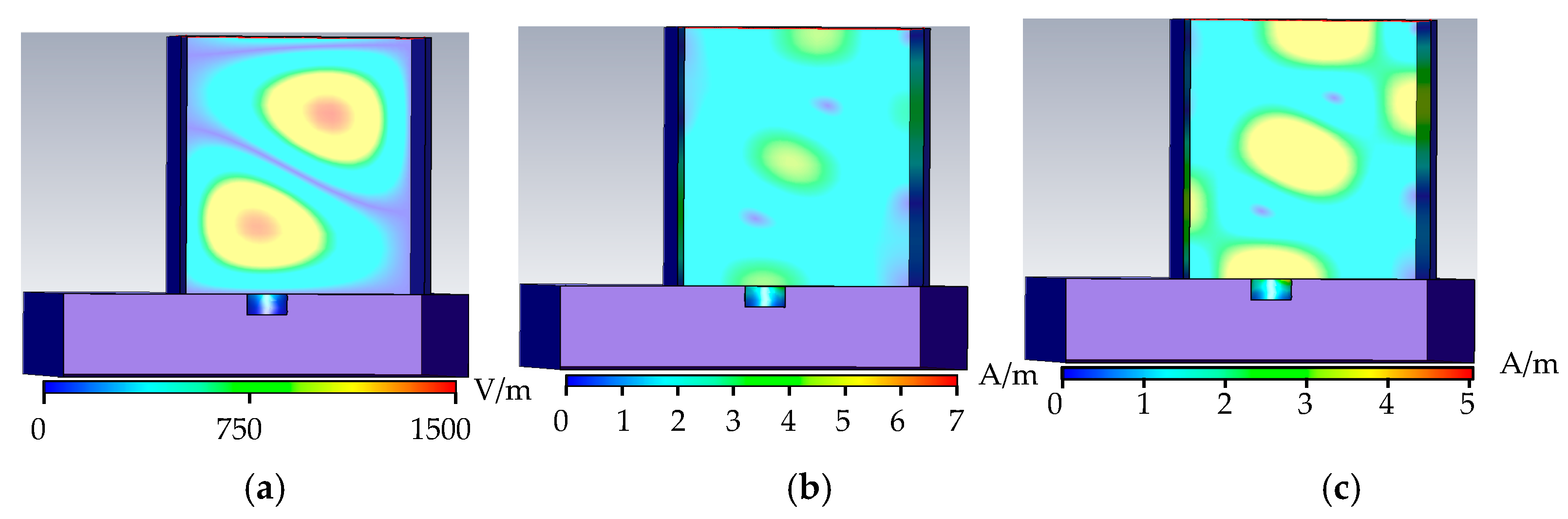
| No Defect | Crack | Triangular Prism | Trapezoid | |
|---|---|---|---|---|
| E (V/m) | 1396.51 | 1401.97 | 2289.77 | 2594.5 |
| H (A/m) | 3.31 | 3.98 | 5.24 | 6.27 |
| J (A/m) | 3.31 | 3.97 | 4.86 | 5.86 |
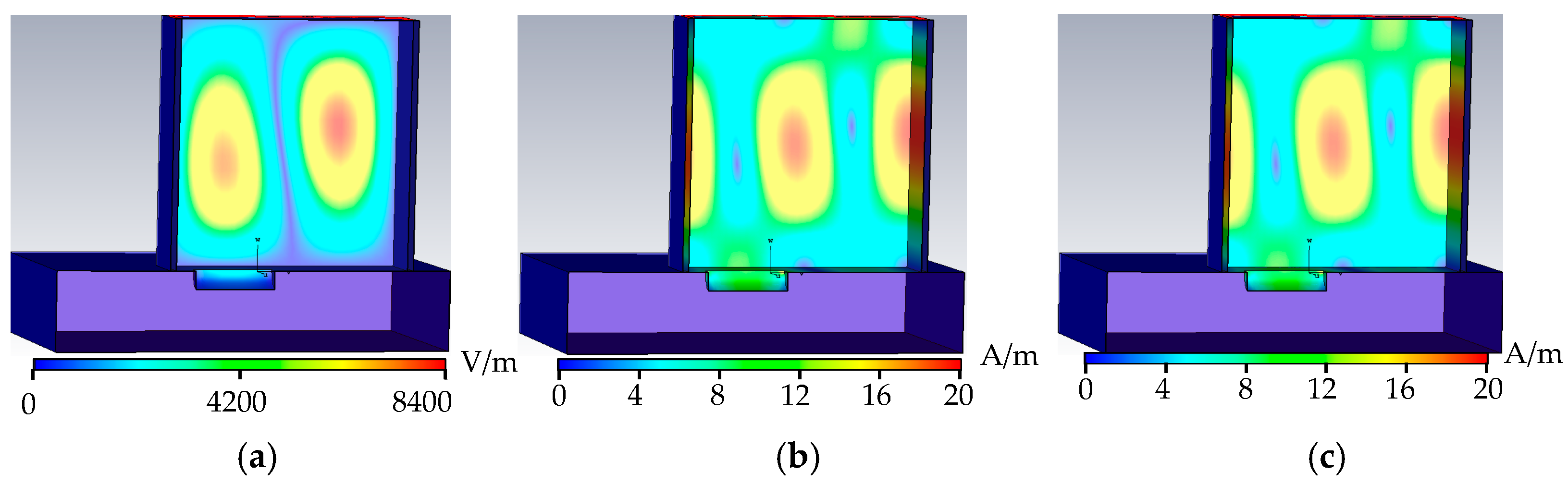
| Cone | Hemisphere | Cylindrical | Semi-Cylindrical | |
|---|---|---|---|---|
| E (V/m) | 1512.09 | 1553.4 | 1696.05 | 8389.74 |
| H (A/m) | 4.63 | 5.89 | 6.58 | 19.73 |
| J (A/m) | 4.12 | 4.43 | 4.67 | 19.67 |
Publisher’s Note: MDPI stays neutral with regard to jurisdictional claims in published maps and institutional affiliations. |
© 2022 by the authors. Licensee MDPI, Basel, Switzerland. This article is an open access article distributed under the terms and conditions of the Creative Commons Attribution (CC BY) license (https://creativecommons.org/licenses/by/4.0/).
Share and Cite
Shi, M.; Yang, L.; Gao, S.; Wang, G. Metal Surface Defect Detection Method Based on TE01 Mode Microwave. Sensors 2022, 22, 4848. https://doi.org/10.3390/s22134848
Shi M, Yang L, Gao S, Wang G. Metal Surface Defect Detection Method Based on TE01 Mode Microwave. Sensors. 2022; 22(13):4848. https://doi.org/10.3390/s22134848
Chicago/Turabian StyleShi, Meng, Lijian Yang, Songwei Gao, and Guoqing Wang. 2022. "Metal Surface Defect Detection Method Based on TE01 Mode Microwave" Sensors 22, no. 13: 4848. https://doi.org/10.3390/s22134848