
Prediction of Lower Extremity Multi-Joint Angles during Overground Walking by Using a Single IMU with a Low Frequency Based on an LSTM Recurrent Neural Network

 , , and
Abstract
:1. Introduction
2. Materials and Methods
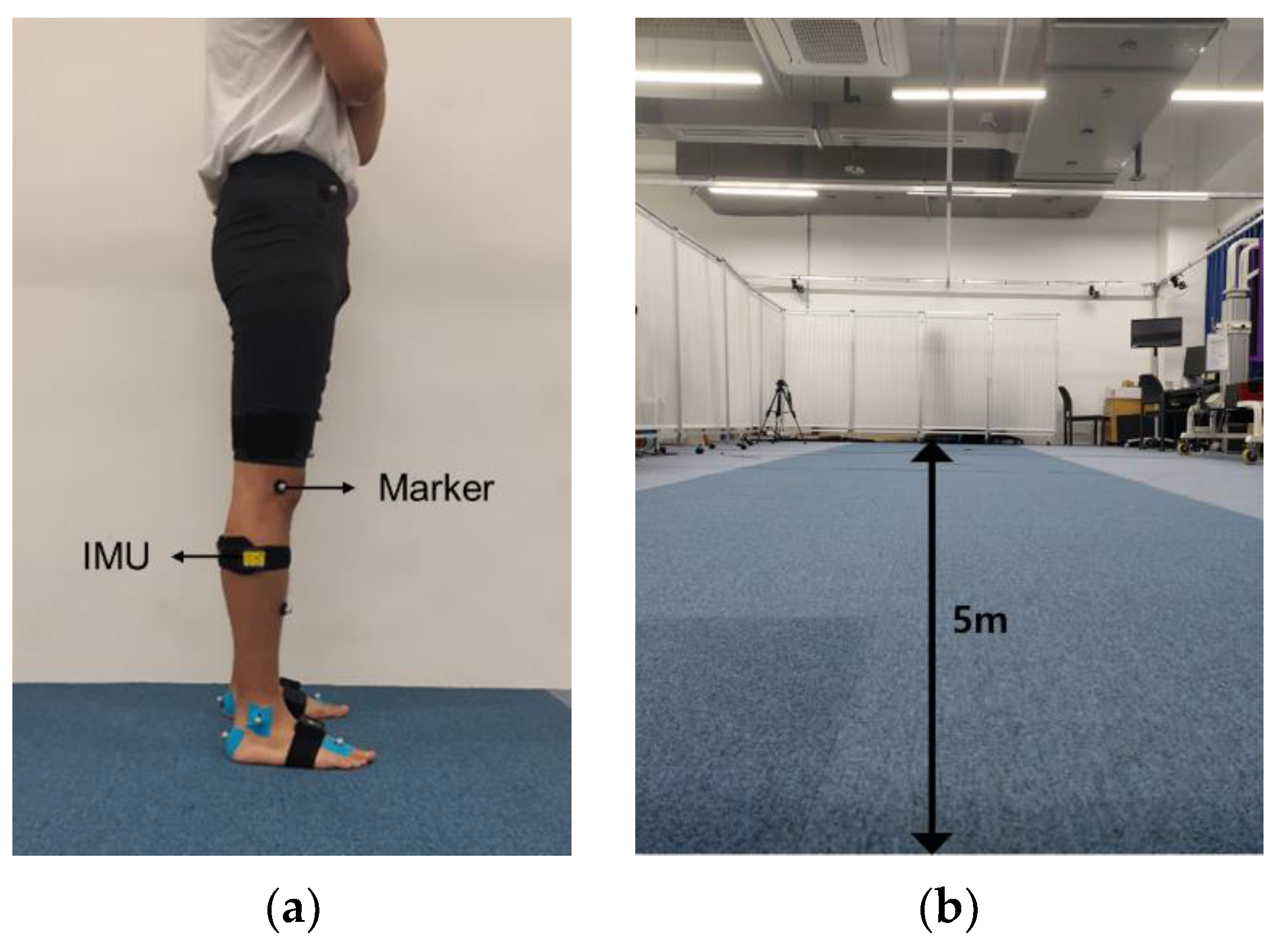
2.1. Experimental Equipment and Protocol
2.2. Data Preprocessing
2.2.1. Data Resampling and Filtering
2.2.2. Feature Extraction
2.3. Deep Learning Model
2.3.1. Background
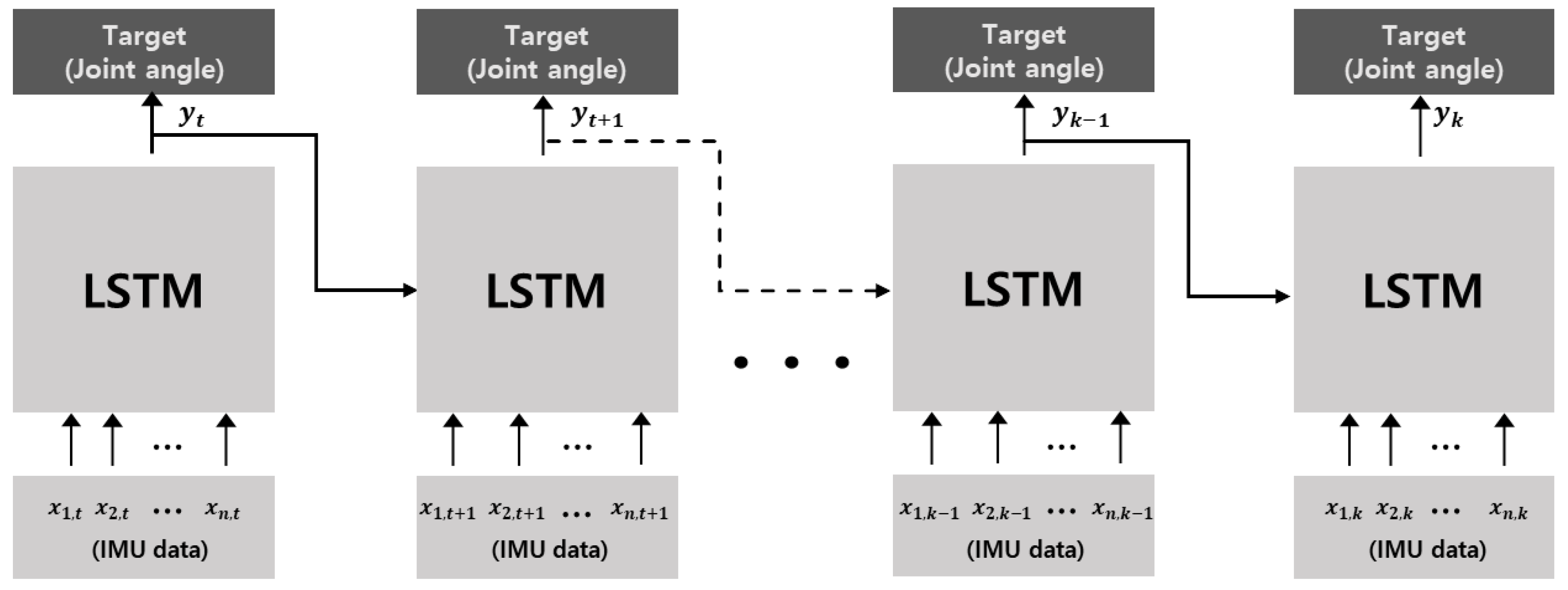
2.3.2. Model Design
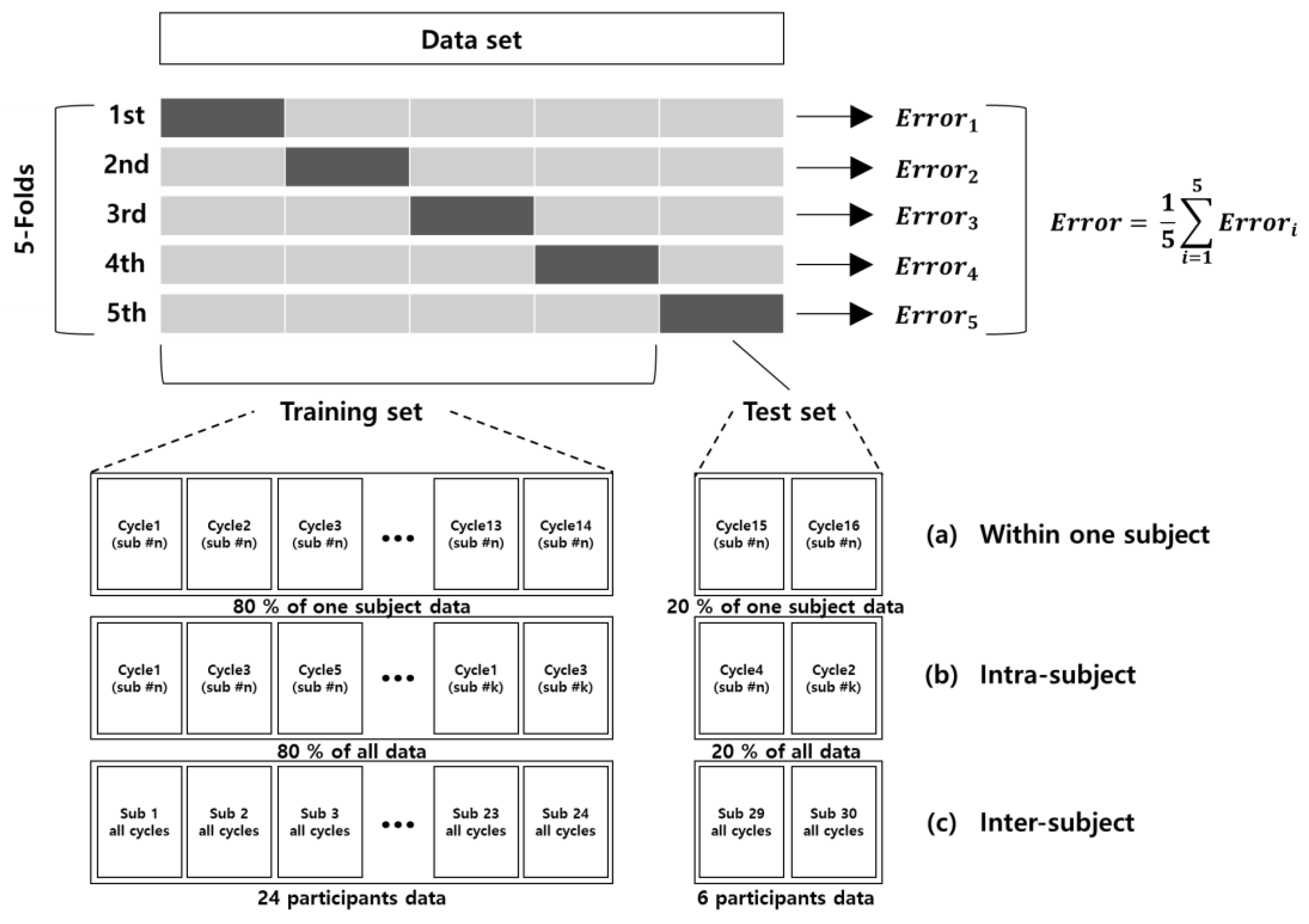
2.4. Data Analysis
3. Results
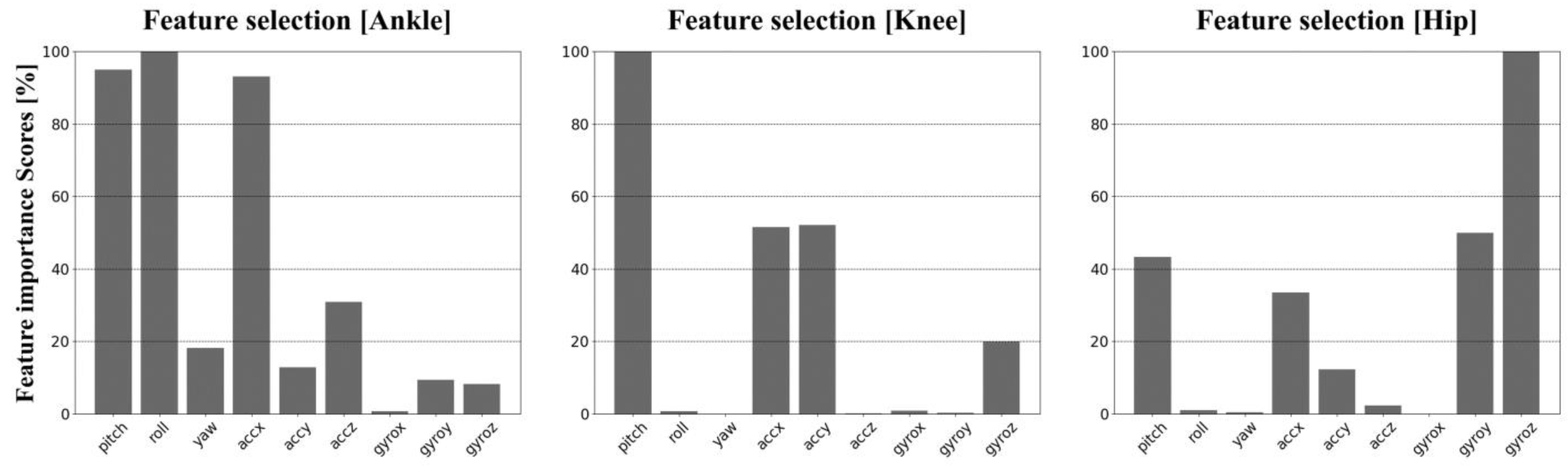
3.1. Feature Extraction
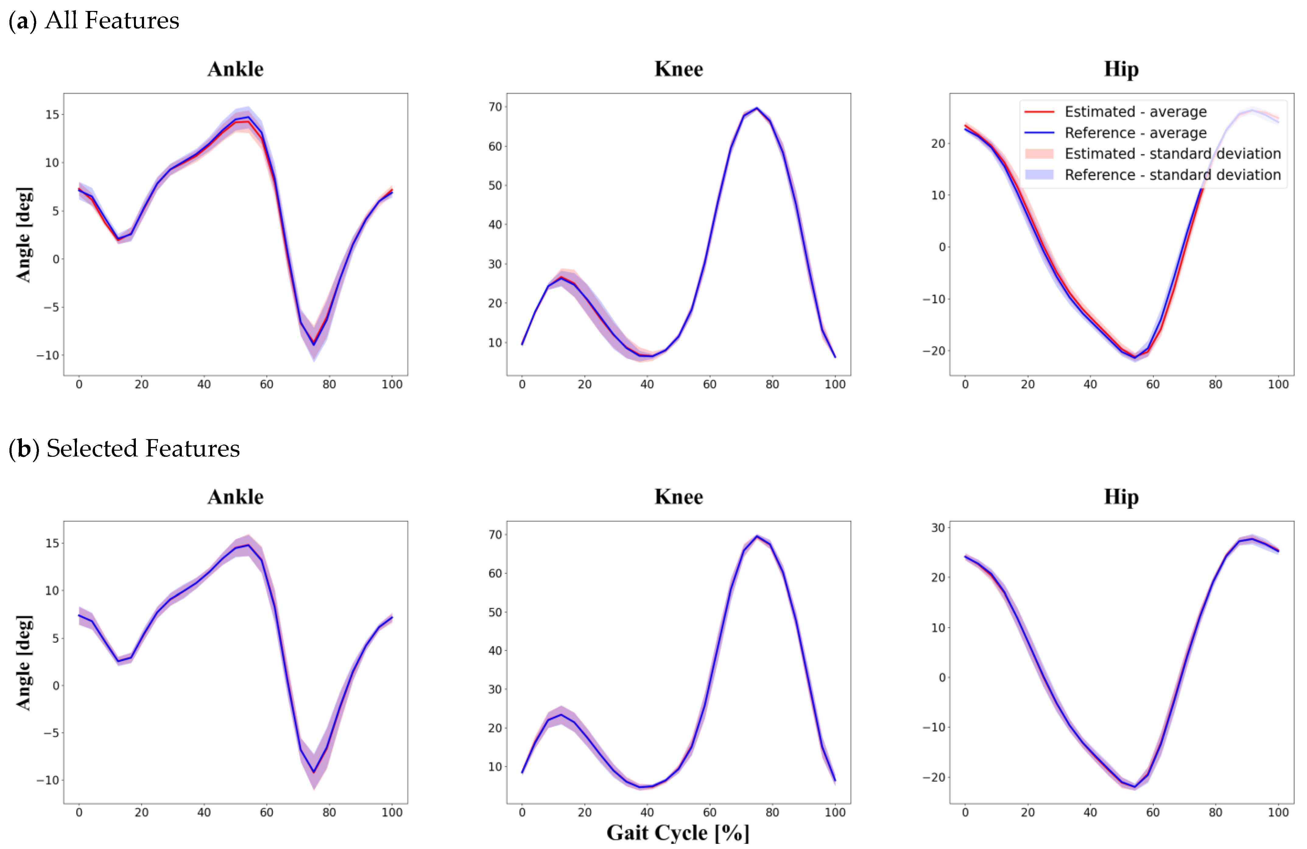
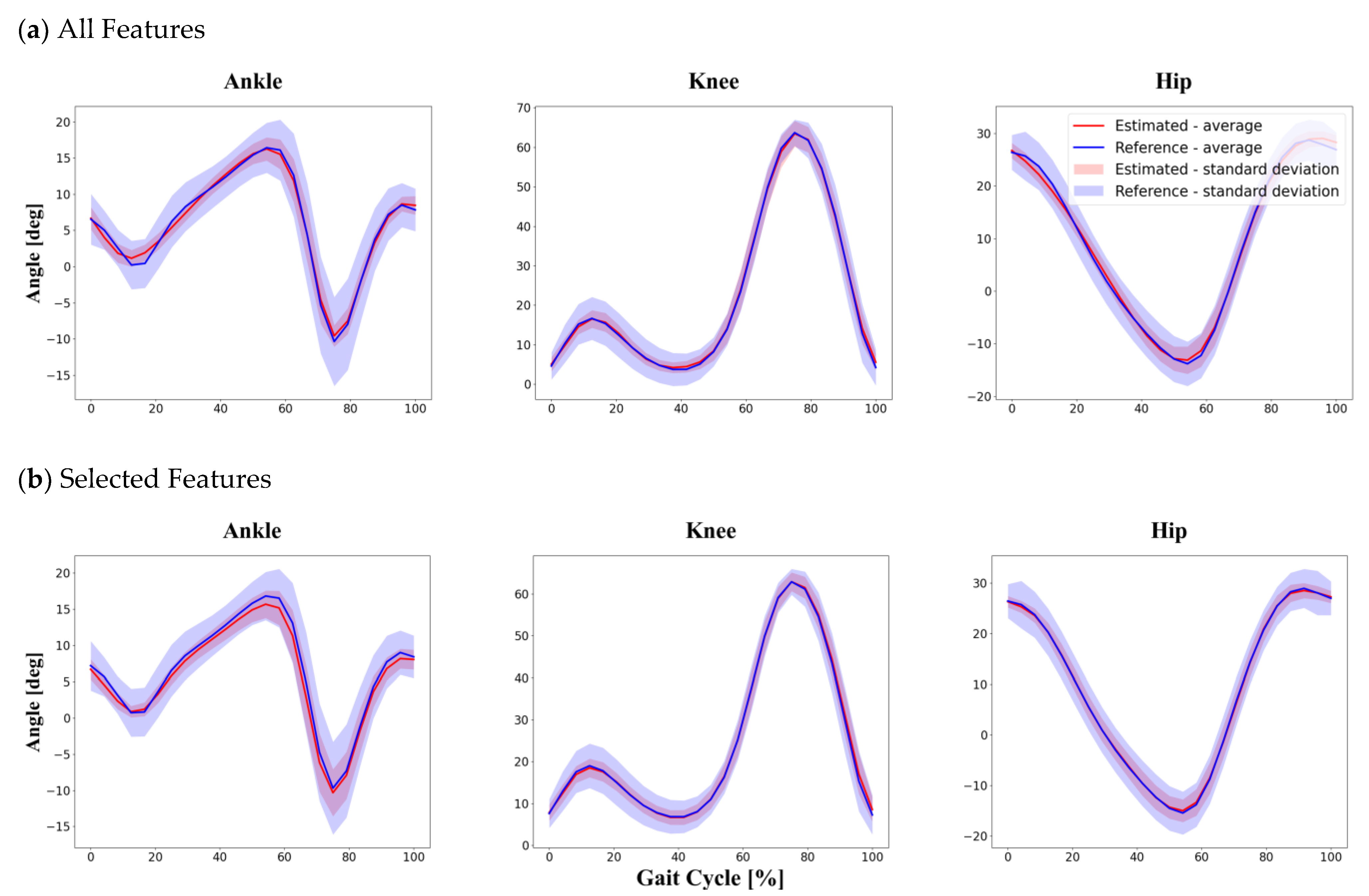
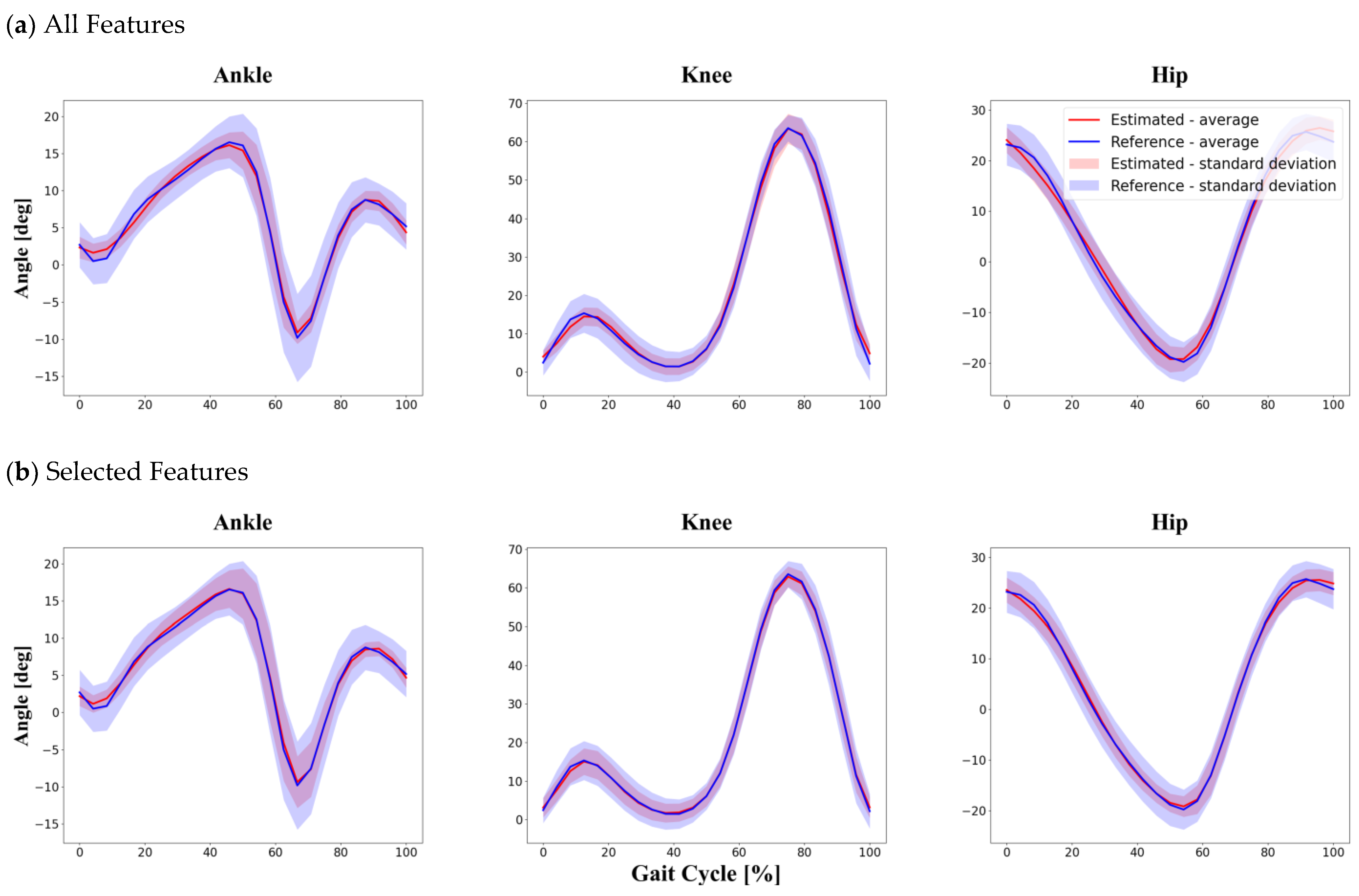
3.2. Estimation of Joint Angles
4. Discussion
5. Conclusions
Author Contributions
Funding
Institutional Review Board Statement
Informed Consent Statement
Data Availability Statement
Conflicts of Interest
References
- Baldwin, R.; Bobovych, S.; Robucci, R.; Patel, C.; Banerjee, N. Gait analysis for fall prediction using hierarchical textile-based capacitive sensor arrays. In Proceedings of the 2015 Design, Automation & Test in Europe Conference & Exhibition (DATE), Grenoble, France, 9–13 March 2015; pp. 1293–1298. [Google Scholar]
- Schache, A.G.; Blanch, P.D.; Rath, D.A.; Wrigley, T.V.; Bennell, K.L. Are anthropometric and kinematic parameters of the lumbo-pelvic-hip complex related to running injuries? Res. Sports Med. 2005, 13, 127–147. [Google Scholar] [CrossRef] [PubMed]
- Messier, S.P.; Legault, C.; Schoenlank, C.R.; Newman, J.J.; Martin, D.F.; De Vita, P. Risk factors and mechanisms of knee injury in runners. Med. Sci. Sports Exerc. 2008, 40, 1873–1879. [Google Scholar] [CrossRef]
- McClelland, J.A.; Webster, K.E.; Feller, J.A. Gait analysis of patients following total knee replacement: A systematic review. Knee 2007, 14, 253–263. [Google Scholar] [CrossRef]
- Anouchi, Y.S.; McShane, M.; Kelly, F., Jr.; Elting, J.; Stiehl, J. Range of motion in total knee replacement. Clin. Orthop Relat Res. 1996, 331, 87–92. [Google Scholar] [CrossRef] [PubMed] [Green Version]
- Dicharry, J. Kinematics and kinetics of gait: From lab to clinic. Clin. Sports Med. 2010, 29, 347–364. [Google Scholar] [CrossRef] [PubMed]
- Folland, J.P.; Allen, S.J.; Black, M.I.; Handsaker, J.C.; Forrester, S.E. Running Technique is an Important Component of Running Economy and Performance. Med. Sci. Ence Sports Exerc. 2017, 49, 1412–1423. [Google Scholar] [CrossRef] [PubMed] [Green Version]
- Wahid, F.; Begg, R.K.; Hass, C.J.; Halgamuge, S.; Ackland, D.C. Classification of Parkinson’s Disease Gait Using Spatial-Temporal Gait Features. IEEE J. Biomed. Health Inform. 2015, 19, 1794–1802. [Google Scholar] [CrossRef] [PubMed]
- Panero, E.; Digo, E.; Agostini, V.; Gastaldi, L. Comparison of different motion capture setups for gait analysis: Validation of spatio-temporal parameters estimation. In Proceedings of the 2018 IEEE International Symposium on Medical Measurements and Applications (MeMeA), Rome, Italy, 11–13 June 2018; pp. 1–6. [Google Scholar]
- Mundt, M.; Thomsen, W.; Witter, T.; Koeppe, A.; David, S.; Bamer, F.; Potthast, W.; Markert, B. Prediction of lower limb joint angles and moments during gait using artificial neural networks. Med. Biol. Eng. Comput. 2020, 58, 211–225. [Google Scholar] [CrossRef]
- Ho, S.; Mohtadi, A.; Daud, K.; Leonards, U.; Handy, T.C. Using smartphone accelerometry to assess the relationship between cognitive load and gait dynamics during outdoor walking. Sci. Rep. 2019, 9, 3119. [Google Scholar] [CrossRef] [Green Version]
- Zhao, H.; Wang, Z.; Qiu, S.; Shen, Y.; Wang, J. IMU-based gait analysis for rehabilitation assessment of patients with gait disorders. In Proceedings of the 2017 4th International Conference on Systems and Informatics (ICSAI), Hangzhou, China, 11–13 November 2017; pp. 622–626. [Google Scholar]
- Fusca, M.; Negrini, F.; Perego, P.; Magoni, L.; Molteni, F.; Andreoni, G. Validation of a Wearable IMU System for Gait Analysis: Protocol and Application to a New System. Appl. Sci.-Basel 2018, 8, 1167. [Google Scholar] [CrossRef] [Green Version]
- Zhou, L.; Tunca, C.; Fischer, E.; Brahms, C.M.; Ersoy, C.; Granacher, U.; Arnrich, B. Validation of an IMU gait analysis algorithm for gait monitoring in daily life situations. In Proceedings of the 2020 42nd Annual International Conference of the IEEE Engineering in Medicine & Biology Society (EMBC), Montreal, QC, Canada, 20–24 July 2020; pp. 4229–4232. [Google Scholar]
- Vargas-Valencia, L.S.; Elias, A.; Rocon, E.; Bastos-Filho, T.; Frizera, A. An IMU-to-Body Alignment Method Applied to Human Gait Analysis. Sensors 2016, 16, 2090. [Google Scholar] [CrossRef] [Green Version]
- Seel, T.; Raisch, J.; Schauer, T. IMU-based joint angle measurement for gait analysis. Sensors 2014, 14, 6891–6909. [Google Scholar] [CrossRef] [Green Version]
- Lim, H.; Kim, B.; Park, S. Prediction of Lower Limb Kinetics and Kinematics during Walking by a Single IMU on the Lower Back Using Machine Learning. Sensors 2020, 20, 130. [Google Scholar] [CrossRef] [Green Version]
- Gholami, M.; Napier, C.; Menon, C. Estimating Lower Extremity Running Gait Kinematics with a Single Accelerometer: A Deep Learning Approach. Sensors 2020, 20, 2939. [Google Scholar] [CrossRef]
- Alton, F.; Baldey, L.; Caplan, S.; Morrissey, M.C. A kinematic comparison of overground and treadmill walking. Clin. Biomech 1998, 13, 434–440. [Google Scholar] [CrossRef]
- Riley, P.O.; Paolini, G.; Della Croce, U.; Paylo, K.W.; Kerrigan, D.C. A kinematic and kinetic comparison of overground and treadmill walking in healthy subjects. Gait Posture 2007, 26, 17–24. [Google Scholar] [CrossRef]
- Lee, S.J.; Hidler, J. Biomechanics of overground vs. treadmill walking in healthy individuals. J. Appl. Physiol. (1985) 2008, 104, 747–755. [Google Scholar] [CrossRef]
- Tobola, A.; Streit, F.J.; Espig, C.; Korpok, O.; Sauter, C.; Lang, N.; Schmitz, B.; Hofmann, C.; Struck, M.; Weigand, C. Sampling rate impact on energy consumption of biomedical signal processing systems. In Proceedings of the 2015 IEEE 12th International Conference on Wearable and Implantable Body Sensor Networks (BSN), Cambridge, MA, USA, 9–12 June 2015; pp. 1–6. [Google Scholar]
- Krause, A.; Ihmig, M.; Rankin, E.; Leong, D.; Gupta, S.; Siewiorek, D.; Smailagic, A.; Deisher, M.; Sengupta, U. Trading off prediction accuracy and power consumption for context-aware wearable computing. In Proceedings of the Ninth IEEE International Symposium on Wearable Computers (ISWC’05), Osaka, Japan, 18–21 October 2005; pp. 20–26. [Google Scholar]
- Allseits, E.K.; Agrawal, V.; Prasad, A.; Bennett, C.; Kim, K.J. Characterizing the Impact of Sampling Rate and Filter Design on the Morphology of Lower Limb Angular Velocities. IEEE Sens. J. 2019, 19, 4115–4122. [Google Scholar] [CrossRef]
- de Vries, A.; Zwerver, J.; Diercks, R.; Tak, I.; van Berkel, S.; van Cingel, R.; van der Worp, H.; van den Akker-Scheek, I. Effect of patellar strap and sports tape on pain in patellar tendinopathy: A randomized controlled trial. Scand. J. Med. Sci. Sports 2016, 26, 1217–1224. [Google Scholar] [CrossRef]
- de Vries, A.J.; van den Akker-Scheek, I.; Diercks, R.L.; Zwerver, J.; van der Worp, H. The effect of a patellar strap on knee joint proprioception in healthy participants and athletes with patellar tendinopathy. J. Sci. Med. Sport 2016, 19, 278–282. [Google Scholar] [CrossRef]
- Collins, T.D.; Ghoussayni, S.N.; Ewins, D.J.; Kent, J.A. A six degrees-of-freedom marker set for gait analysis: Repeatability and comparison with a modified Helen Hayes set. Gait Posture 2009, 30, 173–180. [Google Scholar] [CrossRef]
- Kadaba, M.P.; Ramakrishnan, H.K.; Wootten, M.E.; Gainey, J.; Gorton, G.; Cochran, G.V. Repeatability of kinematic, kinetic, and electromyographic data in normal adult gait. J. Orthop Res. 1989, 7, 849–860. [Google Scholar] [CrossRef]
- Erdem, N.S.; Ersoy, C.; Tunca, C. Gait analysis using smartwatches. In Proceedings of the 2019 IEEE 30th International Symposium on Personal, Indoor and Mobile Radio Communications (PIMRC Workshops), Istanbul, Turkey, 8–11 September 2019; pp. 1–6. [Google Scholar]
- Kuhn, M.; Johnson, K. Applied Predictive Modeling; Springer: Berlin/Heidelberg, Germany, 2013; Volume 26. [Google Scholar]
- Liu, P.; Qiu, X.; Huang, X. Recurrent neural network for text classification with multi-task learning. arXiv 2016, arXiv:1605.05101. [Google Scholar]
- Parascandolo, G.; Huttunen, H.; Virtanen, T. Recurrent neural networks for polyphonic sound event detection in real life recordings. In Proceedings of the 2016 IEEE international Conference on Acoustics, Speech and Signal Processing (ICASSP), Shanghai, China, 20–25 March 2016; pp. 6440–6444. [Google Scholar]
- Sutskever, I.; Martens, J.; Hinton, G.E. Generating text with recurrent neural networks. In Proceedings of the ICML, Washington, DC, USA, 28 June–2 July 2011. [Google Scholar]
- Valentini-Botinhao, C.; Wang, X.; Takaki, S.; Yamagishi, J. Investigating RNN-based speech enhancement methods for noise-robust Text-to-Speech. In Proceedings of the SSW, Sunnyvale, CA, USA, 13–15 September 2016; pp. 146–152. [Google Scholar]
- Hochreiter, S. The vanishing gradient problem during learning recurrent neural nets and problem solutions. Int. J. Uncertain. Fuzziness Knowl. -Based Syst. 1998, 6, 107–116. [Google Scholar] [CrossRef] [Green Version]
- Hochreiter, S.; Schmidhuber, J. Long short-term memory. Neural Comput 1997, 9, 1735–1780. [Google Scholar] [CrossRef]
- Gers, F.A.; Schraudolph, N.N.; Schmidhuber, J. Learning precise timing with LSTM recurrent networks. J. Mach. Learn. Res. 2002, 3, 115–143. [Google Scholar]
- Kingma, D.P.; Ba, J. Adam: A method for stochastic optimization. arXiv 2014, arXiv:1412.6980. [Google Scholar]
- Alexander, D.L.; Tropsha, A.; Winkler, D.A. Beware of R(2): Simple, Unambiguous Assessment of the Prediction Accuracy of QSAR and QSPR Models. J. Chem. Inf. Model. 2015, 55, 1316–1322. [Google Scholar] [CrossRef] [PubMed] [Green Version]
- Dorschky, E.; Nitschke, M.; Seifer, A.K.; van den Bogert, A.J.; Eskofier, B.M. Estimation of gait kinematics and kinetics from inertial sensor data using optimal control of musculoskeletal models. J. Biomech. 2019, 95, 109278. [Google Scholar] [CrossRef] [PubMed]
- Gholami, M.; Rezaei, A.; Cuthbert, T.J.; Napier, C.; Menon, C. Lower Body Kinematics Monitoring in Running Using Fabric-Based Wearable Sensors and Deep Convolutional Neural Networks. Sensors 2019, 19, 5325. [Google Scholar] [CrossRef] [PubMed] [Green Version]
- Hollander, K.; Petersen, E.; Zech, A.; Hamacher, D. Effects of barefoot vs. shod walking during indoor and outdoor conditions in younger and older adults. Gait Posture, 2021; In Press. [Google Scholar] [CrossRef]
- Schmitt, A.C.; Baudendistel, S.T.; Lipat, A.L.; White, T.A.; Raffegeau, T.E.; Hass, C.J. Walking indoors, outdoors, and on a treadmill: Gait differences in healthy young and older adults. Gait Posture 2021, 90, 468–474. [Google Scholar] [CrossRef]
- Cho, S.H.; Park, J.M.; Kwon, O.Y. Gender differences in three dimensional gait analysis data from 98 healthy Korean adults. Clin. Biomech 2004, 19, 145–152. [Google Scholar] [CrossRef]
- Schloemer, S.A.; Thompson, J.A.; Silder, A.; Thelen, D.G.; Siston, R.A. Age-Related Differences in Gait Kinematics, Kinetics, and Muscle Function: A Principal Component Analysis. Ann. Biomed. Eng. 2017, 45, 695–710. [Google Scholar] [CrossRef]
- McClelland, J.A.; Webster, K.E.; Feller, J.A.; Menz, H.B. Knee kinematics during walking at different speeds in people who have undergone total knee replacement. Knee 2011, 18, 151–155. [Google Scholar] [CrossRef]
- Chen, G.; Patten, C.; Kothari, D.H.; Zajac, F.E. Gait differences between individuals with post-stroke hemiparesis and non-disabled controls at matched speeds. Gait Posture 2005, 22, 51–56. [Google Scholar] [CrossRef]


| Hyperparameters | Values |
|---|---|
| Number of layers | 1 |
| Batch size | 256 |
| Hidden size | 50 |
| Optimizer | Adam |
| Learning rate | 0.001 |
| Sequence length | 5 |
| Number of epochs | 500 |
| Activation function | Tanh |
| Ankle Joint | Knee Joint | Hip Joint | ||
|---|---|---|---|---|
| All Features | 0.96 | 0.99 | 0.97 | |
| RMSE () | 0.42 | 0.36 | 0.83 | |
| NRMSE (%) | 1.43 | 0.57 | 1.59 | |
| Selected Features | 0.98 | 0.99 | 0.98 | |
| RMSE () | 0.14 | 0.15 | 0.47 | |
| NRMSE (%) | 0.54 | 0.24 | 0.91 | |
| Ankle Joint | Knee Joint | Hip Joint | ||
|---|---|---|---|---|
| All Features | 0.73 | 0.89 | 0.90 | |
| RMSE () | 3.96 | 6.34 | 5.47 | |
| NRMSE (%) | 8.52 | 9.30 | 9.01 | |
| Selected Features | 0.83 | 0.92 | 0.90 | |
| RMSE () | 3.06 | 5.76 | 4.80 | |
| NRMSE (%) | 7.21 | 6.70 | 8.66 | |
| Ankle Joint | Knee Joint | Hip Joint | ||
|---|---|---|---|---|
| All Features | 0.62 | 0.87 | 0.84 | |
| RMSE () | 5.15 | 8.14 | 7.49 | |
| NRMSE (%) | 12.2 | 11.01 | 10.97 | |
| Selected Features | 0.74 | 0.89 | 0.86 | |
| RMSE () | 4.35 | 7.00 | 6.19 | |
| NRMSE (%) | 9.87 | 9.10 | 9.74 | |
Publisher’s Note: MDPI stays neutral with regard to jurisdictional claims in published maps and institutional affiliations. |
© 2021 by the authors. Licensee MDPI, Basel, Switzerland. This article is an open access article distributed under the terms and conditions of the Creative Commons Attribution (CC BY) license (https://creativecommons.org/licenses/by/4.0/).
Share and Cite
Sung, J.; Han, S.; Park, H.; Cho, H.-M.; Hwang, S.; Park, J.W.; Youn, I. Prediction of Lower Extremity Multi-Joint Angles during Overground Walking by Using a Single IMU with a Low Frequency Based on an LSTM Recurrent Neural Network. Sensors 2022, 22, 53. https://doi.org/10.3390/s22010053
Sung J, Han S, Park H, Cho H-M, Hwang S, Park JW, Youn I. Prediction of Lower Extremity Multi-Joint Angles during Overground Walking by Using a Single IMU with a Low Frequency Based on an LSTM Recurrent Neural Network. Sensors. 2022; 22(1):53. https://doi.org/10.3390/s22010053
Chicago/Turabian StyleSung, Joohwan, Sungmin Han, Heesu Park, Hyun-Myung Cho, Soree Hwang, Jong Woong Park, and Inchan Youn. 2022. "Prediction of Lower Extremity Multi-Joint Angles during Overground Walking by Using a Single IMU with a Low Frequency Based on an LSTM Recurrent Neural Network" Sensors 22, no. 1: 53. https://doi.org/10.3390/s22010053