Author Contributions
Formal analysis, visualization and writing—original draft preparation, J.P.V.; writing—review and editing, A.W. and K.I.W.; data curation, A.W.; investigation, J.P.V., A.W. and K.I.W.; conceptualization and methodology, J.P.V., A.W., K.I.W., P.K., K.I. and D.F.; software, J.P.V., K.I. and T.S.; validation, A.W. and D.F.; resources, K.I. and D.F.; review P.K., K.I., T.S., F.W. and D.F.; supervision, P.K., T.S., F.W. and D.F.; project administration, K.I., K.I.W., P.K. and D.F.; funding acquisition, K.I., K.I.W., P.K., D.F. and F.W. All authors have read and agreed to the published version of the manuscript.
Figure 1.
An avatar which performs movements at a virtual workplace. An exemplary representation of the relevant joint positions for the determination of the joint angle of the elbow flexion.
Figure 1.
An avatar which performs movements at a virtual workplace. An exemplary representation of the relevant joint positions for the determination of the joint angle of the elbow flexion.
Figure 2.
The HTC Vive measurement setup with four base stations and a centrally placed test person with an HMD, two controllers and six trackers.
Figure 2.
The HTC Vive measurement setup with four base stations and a centrally placed test person with an HMD, two controllers and six trackers.
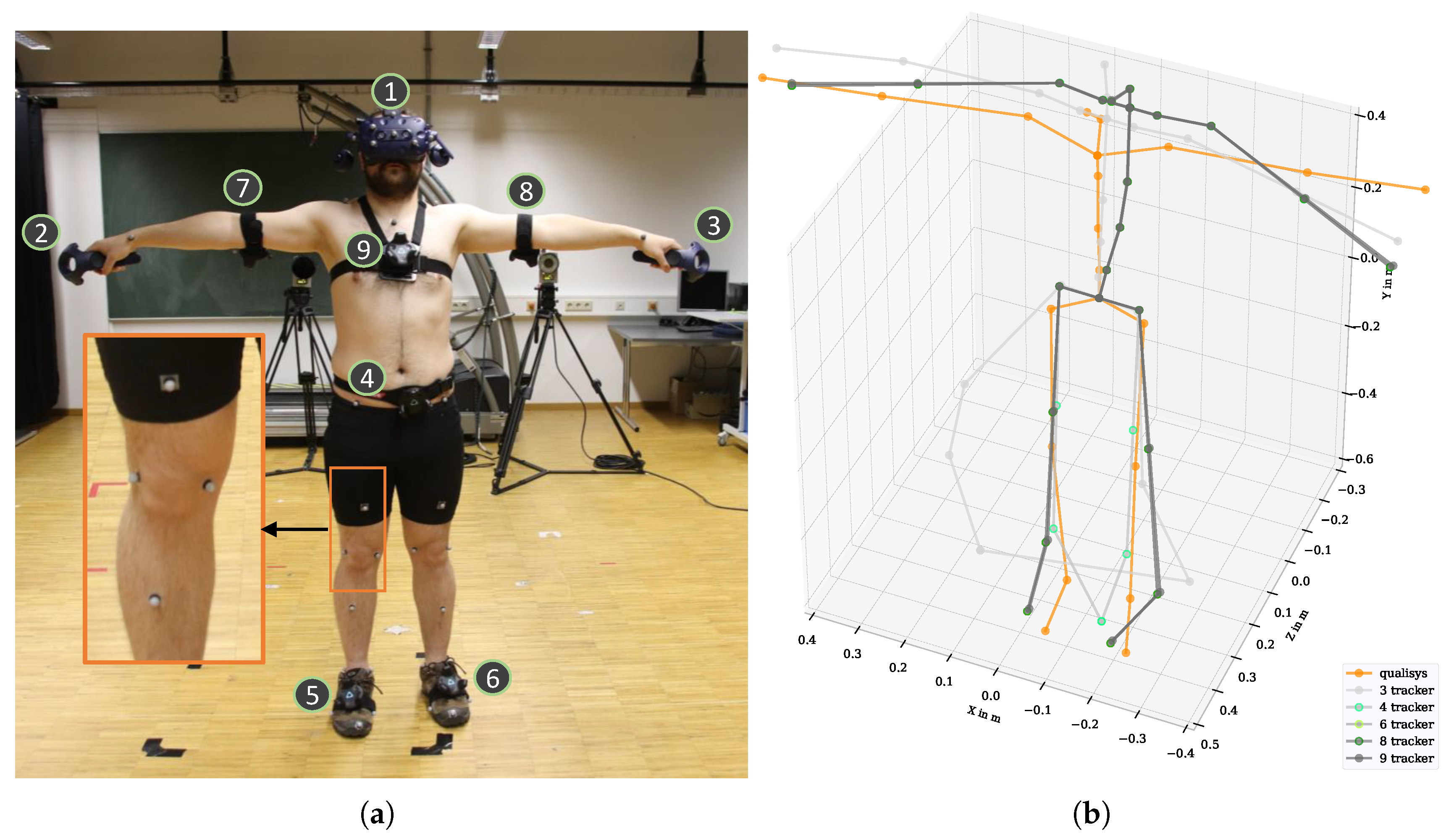
Figure 3.
Setup of simultaneous motion measurements with the Qualisys system and the Vive system with different tracker configurations. (a) A participant in T-position with attached markers for the Qualisys system and Vive trackers, specified with the numbers 1–9. (b) A body skeleton based on the Qualisys system and on different Vive tracker configurations.
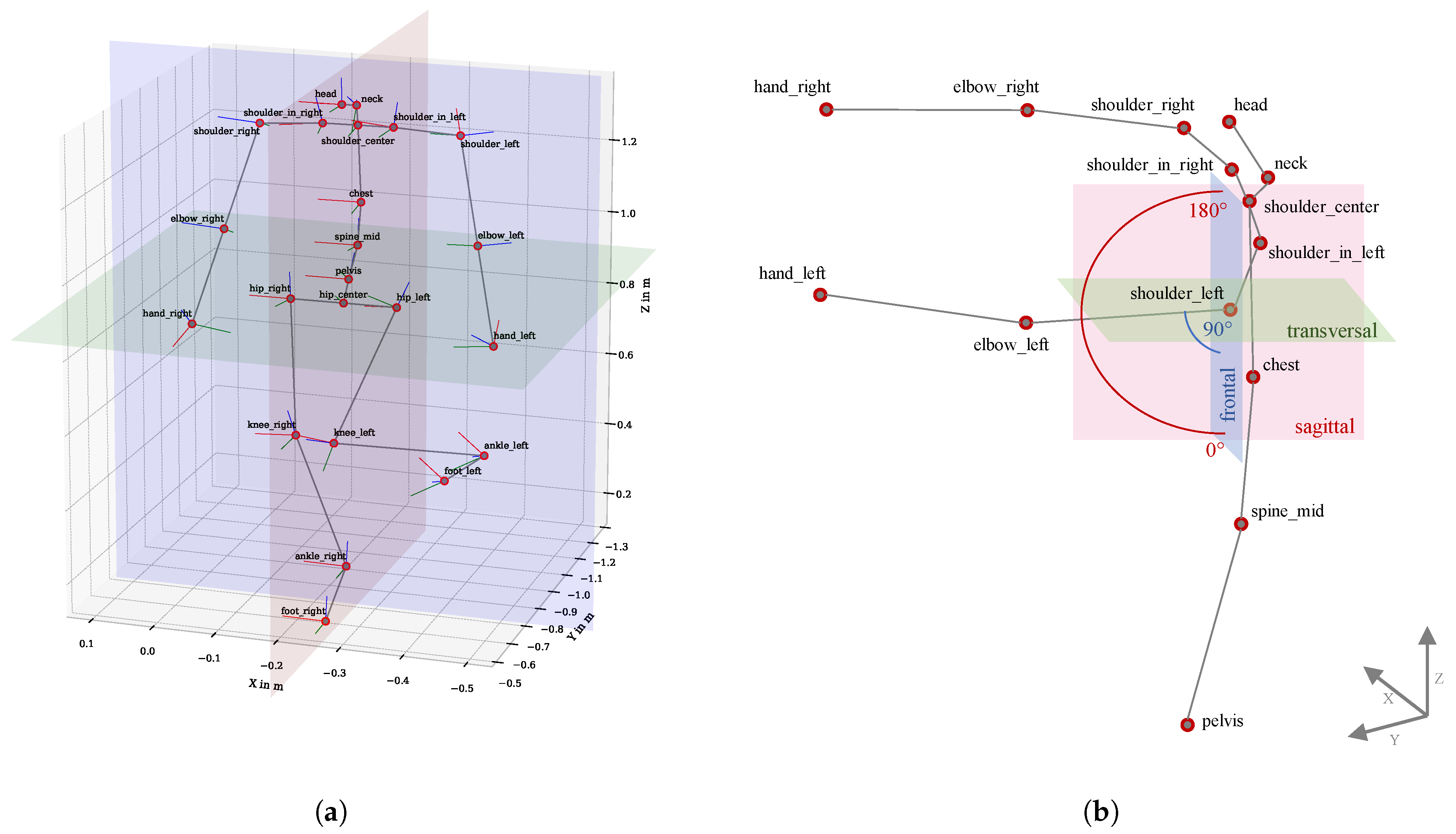
Figure 4.
Method for calculating joint angles. (a) Kinematic data (positions and local coordinate systems based on quaternions) from body posture when standing on one leg while the right hand rotates. Globally plotted body planes: frontal in blue, sagittal in red and transversal in green. (b) An example of the calculation of the left shoulder’s elevation (shoulder_left_elev). The body planes are set locally to the shoulder_left position and orientated using shoulder_center and chest. The elevation angle is calculated with the frontal plane and moves in the sagittal plane.
Figure 5.
Calculation of flexion angles based on three Cartesian joint positions (x, y, z) using the example of left knee flexion.
Figure 5.
Calculation of flexion angles based on three Cartesian joint positions (x, y, z) using the example of left knee flexion.
Figure 6.
Time series of some exemplary selected joint angles. Time segments of the examined movements (01–20) are marked as vertical lines. Start of a movement in blue; end of the movement in red.
Figure 6.
Time series of some exemplary selected joint angles. Time segments of the examined movements (01–20) are marked as vertical lines. Start of a movement in blue; end of the movement in red.
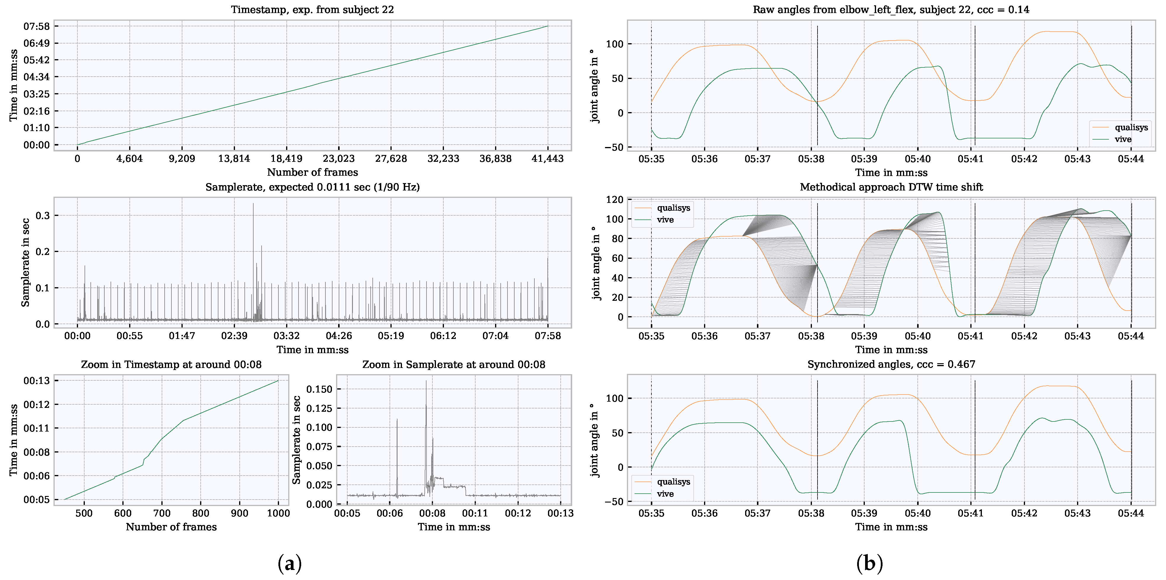
Figure 7.
Cause of the occurring time shifts and demonstration of resynchronization. (a) Sample rate irregularities when recording kinematic data with Vive over an entire measurement per subject for a longer times series and zoomed in. (b) Representation of a time shift between Vive and Qualisys, and the synchronization approach based on DTW; black dotted vertical lines show the segment boundaries of a movement.
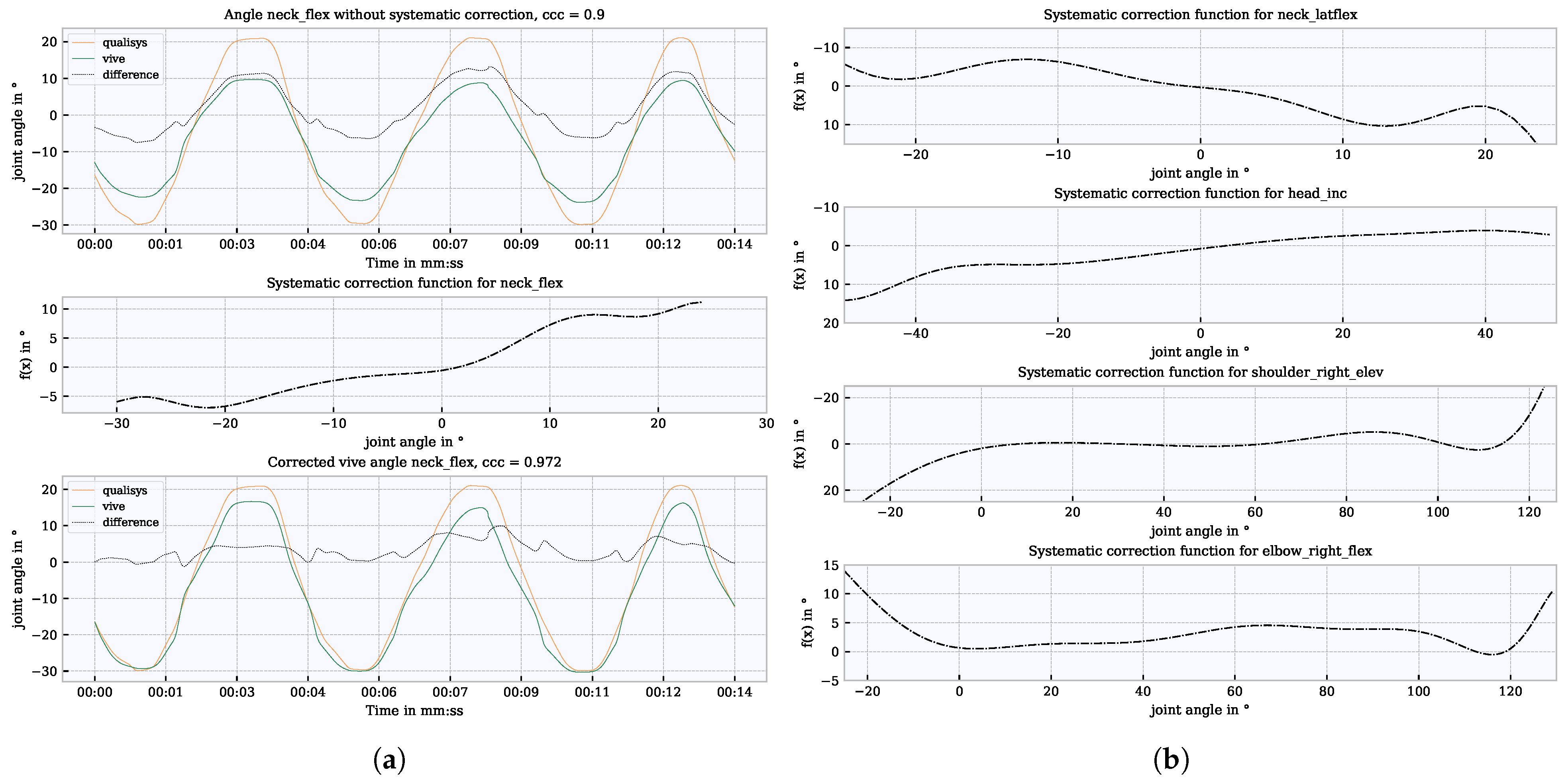
Figure 8.
Systematic correction by polynomial regression function. (a) Systematic differences using the example of neck flexion (upper graph); correction function (middle graph); corrected joint angle (lower graph); (b) further correction functions using the 3 tracker configuration as an example.
Figure 8.
Systematic correction by polynomial regression function. (a) Systematic differences using the example of neck flexion (upper graph); correction function (middle graph); corrected joint angle (lower graph); (b) further correction functions using the 3 tracker configuration as an example.
Figure 9.
Violin representation of the examined joint angles of the Vive tracker configurations 3, 4, 6, 8 and 9 (left violin, green) in comparison to Qualisys (right violin, orange). The quartiles (25%, 50% and 75%) are shown as dotted lines.
Figure 9.
Violin representation of the examined joint angles of the Vive tracker configurations 3, 4, 6, 8 and 9 (left violin, green) in comparison to Qualisys (right violin, orange). The quartiles (25%, 50% and 75%) are shown as dotted lines.
Figure 10.
Comparison of the frequency of occurring angle differences and a comparison of the tracker configurations.
Figure 10.
Comparison of the frequency of occurring angle differences and a comparison of the tracker configurations.
Figure 11.
Concordance correlation coefficient for all studied joint angles and tracker configurations.
Figure 11.
Concordance correlation coefficient for all studied joint angles and tracker configurations.
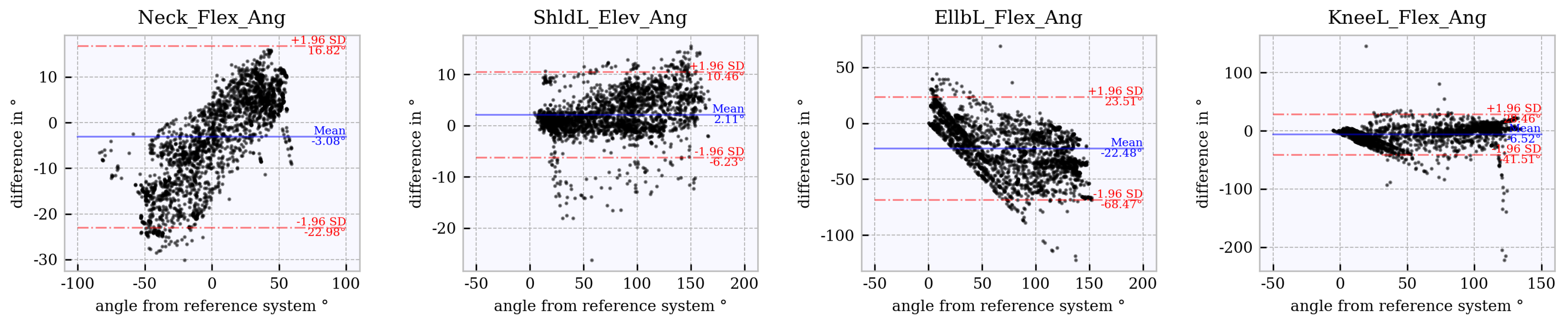
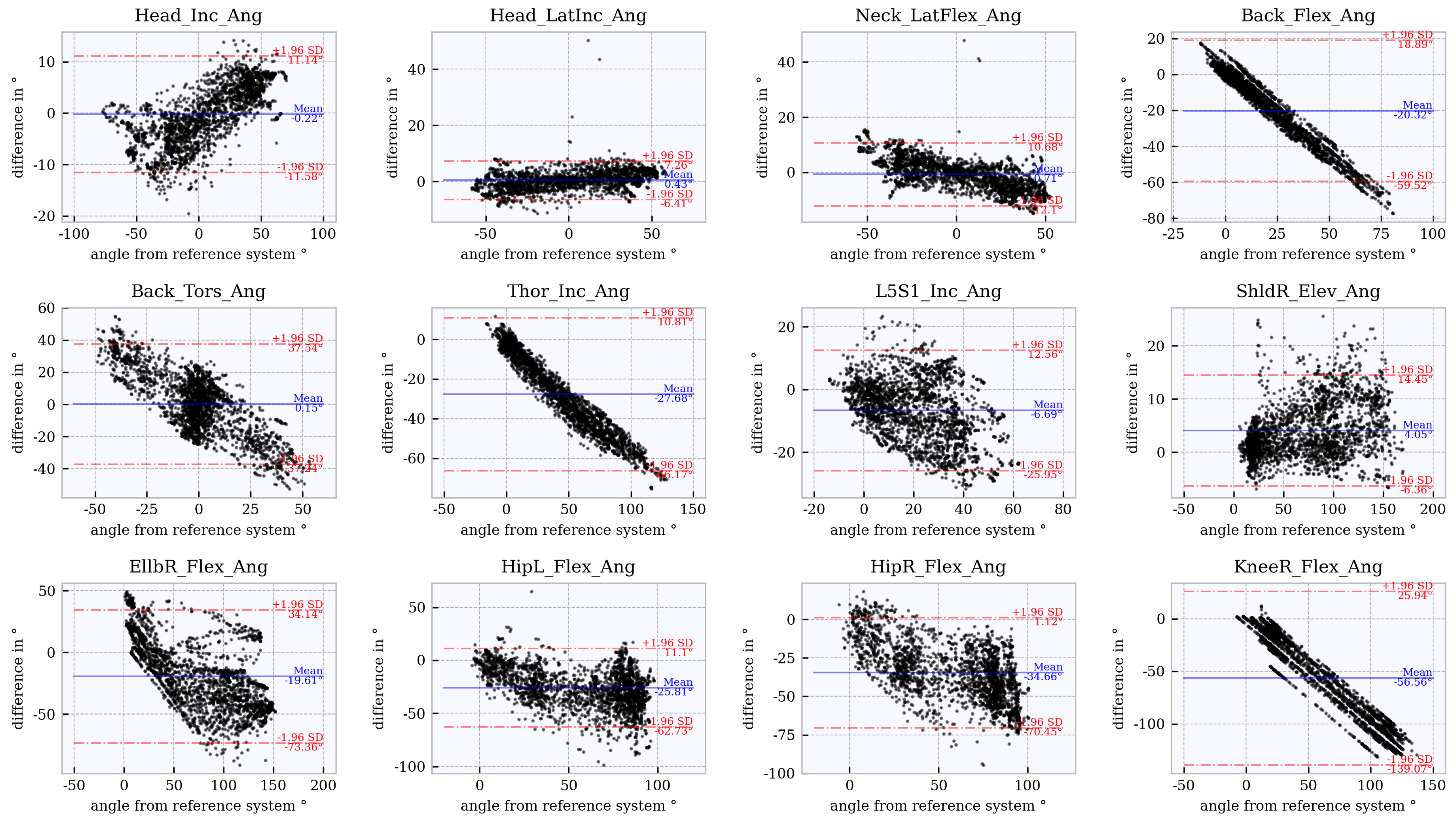
Figure 12.
Bland–Altman plot for tracker configuration 3; x does not show the average of both systems but the joint angles of the reference system, Qualisys.
Figure 12.
Bland–Altman plot for tracker configuration 3; x does not show the average of both systems but the joint angles of the reference system, Qualisys.
Figure 13.
Bland–Altman plot for tracker configuration 4; x does not show the average of both systems but the joint angles of the reference system, Qualisys.
Figure 13.
Bland–Altman plot for tracker configuration 4; x does not show the average of both systems but the joint angles of the reference system, Qualisys.
Figure 14.
Bland–Altman plot for tracker configuration 6; x does not show the average of both systems but the joint angles of the reference system, Qualisys.
Figure 14.
Bland–Altman plot for tracker configuration 6; x does not show the average of both systems but the joint angles of the reference system, Qualisys.
Figure 15.
Bland–Altman plot for tracker configuration 8; x does not show the average of both systems but the joint angles of the reference system, Qualisys.
Figure 15.
Bland–Altman plot for tracker configuration 8; x does not show the average of both systems but the joint angles of the reference system, Qualisys.
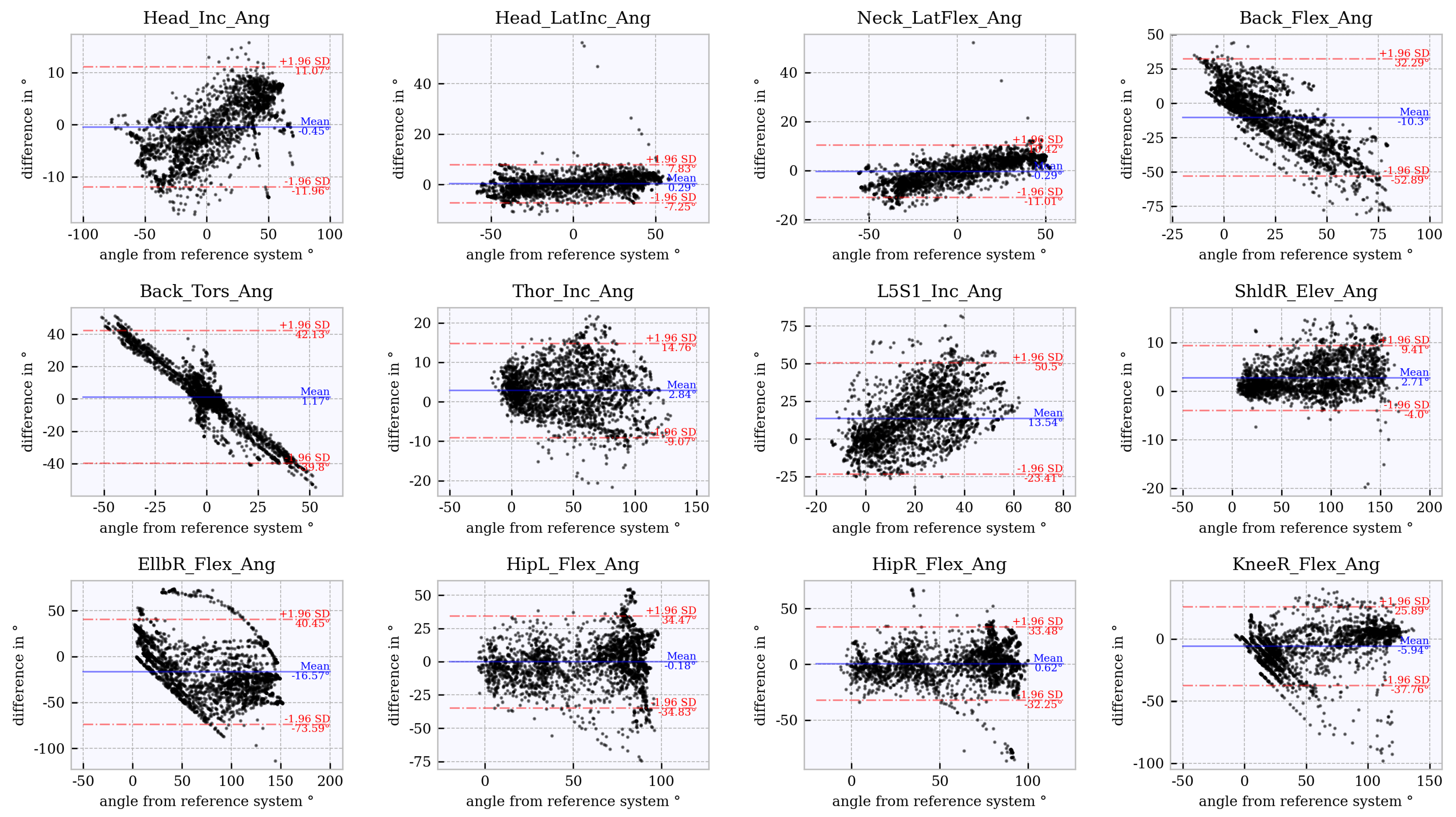
Figure 16.
Bland–Altman plot for tracker configuration 9; x does not show the average of both systems but the joint angles of the reference system, Qualisys.
Figure 16.
Bland–Altman plot for tracker configuration 9; x does not show the average of both systems but the joint angles of the reference system, Qualisys.
Figure 17.
Bland–Altman plot for tracker configuration 3 from WIDAAN; x does not show the average of both systems but the joint angles of the reference system, Qualisys.
Figure 17.
Bland–Altman plot for tracker configuration 3 from WIDAAN; x does not show the average of both systems but the joint angles of the reference system, Qualisys.
Figure 18.
Bland–Altman plot for tracker configuration 9 from WIDAAN; x does not show the average of both systems but the joint angles of the reference system, Qualisys.
Figure 18.
Bland–Altman plot for tracker configuration 9 from WIDAAN; x does not show the average of both systems but the joint angles of the reference system, Qualisys.
Figure 19.
Tracking problems identified by comparing the kinematic data between Qualisys and Vive in tracker configurations 3 and 9. (a) Kinematic differences with a focus on the elbow between tracker and Qualisys (red box). Error based on a rigid knee in trackers (blue box). (b) Illustration of an implausible representation of kinematic data by tracker data.
Figure 20.
Differences caused by time shifts (red box). Differences which are relevant for the accuracy (blue box).
Figure 20.
Differences caused by time shifts (red box). Differences which are relevant for the accuracy (blue box).
Figure 21.
Elbow flexion from to in increments measured with a goniometer. (a) ; (b) ; (c) ; (d) .
Figure 21.
Elbow flexion from to in increments measured with a goniometer. (a) ; (b) ; (c) ; (d) .
Table 1.
Description of the movement segments and associated joint angles.
Table 1.
Description of the movement segments and associated joint angles.
| No. | Description of Movement | Used for Angle |
|---|
|
01 |
head inclination |
head_inc, neck_flex |
|
02 |
head lateral inclination |
head_latinc, neck_latflex |
|
03 |
neck torsion with fixed points approx. at each side | |
|
04 |
bending the torso forward (straight back) |
chest_flex, pelvis_flex |
|
05 |
bending the torso forward (curved back) |
chest_flex, pelvis_flex |
|
06 |
back lateral inclination | |
|
07 |
back torsion with fixed points, approx. | |
|
08–13 |
lifting both arms lateral, frontal |
shoulder_(left, right)_elev |
|
14 |
T-pose with upper arm rotation (drawing circles with hands) | |
|
15 |
elbow flexion (curls) |
elbow_left, right)_flex, elbow_(left, right)_azim |
|
16 |
knee flexion: standing on one leg (right), other lower leg in the air, bent backwards at a angle |
knee_left_flex |
|
17 |
knee flexion: standing on one leg (left), other lower leg in the air, bent backwards at a angle |
knee_right_flex |
|
18 |
squats with outstretched arms, back straight | |
|
19 |
lunge, left leg front, knee flexion , elbow flexion , back torsion to the right, left |
hip_right_flex |
|
20 |
lunge, right leg front, knee flexion , elbow flexion , back torsion to the left, right |
hip_left_flex |
Table 2.
Joint angles with reference to body planes and positions to which the local body planes are orientated.
Table 2.
Joint angles with reference to body planes and positions to which the local body planes are orientated.
|
Joint Angle |
Joint to Body Plane |
Angle in Body Plane |
Positions to which the Body Planes Are Orientated |
|---|
|
neck_flex |
frontal |
saggital |
neck, shoulder_center |
|
neck_latflex |
saggital |
frontal |
shoulder_left, shoulder_right |
|
chest_flex |
frontal |
saggital |
chest, shoulder_center |
|
pelvis_flex |
frontal |
saggital |
hip_center, spine_mid |
|
shoulder_(left, right)_elev |
frontal |
saggital |
shoulder_center, chest |
|
elbow_(left, right)_azim |
saggital |
transversal |
shoulder_center, shoulder_(left, right) |
|
hip_left, right)_flex |
frontal |
saggital |
hip_center, spine_mid |
Table 3.
Differences between the approach used in this paper and WIDAAN.
Table 3.
Differences between the approach used in this paper and WIDAAN.
|
Property |
Approach Paper |
Approach WIDAAN |
|---|
|
Body Model |
individual body dimensions |
body dimensions of “the Dortmunder” |
|
Range of Motion |
dynamic adaptation through systematic correction, outliers possible |
limitation to plausible value ranges, no outliers |
|
Systematic Correction |
systematic offsets are corrected using correction function |
no correction |
Table 4.
Naming of the joint angles, examined using the approach in this paper, and the corresponding joint angles calculated by WIDAAN.
Table 4.
Naming of the joint angles, examined using the approach in this paper, and the corresponding joint angles calculated by WIDAAN.
|
Approach Paper |
Approach WIDAAN |
Description |
|---|
|
head_inc |
Head_Inc_Ang |
back and forward tilt of the head |
|
head_latinc |
Head_LatInc_Ang |
lateral tilt of the head |
|
neck_flex |
Neck_Flex_Ang |
back and forward tilt of the neck |
|
neck_latflex |
Neck_LatFlex_Ang |
lateral tilt of the neck |
|
chest_flex | |
flexion of the spine at chest level |
|
pelvis_flex | |
flexion of the upper body at pelvis level |
|
shoulder_(left, right)_elev |
Shld(L,R)_Elev_Ang |
angle between upper arm and upper body |
|
elbow_left, right)_flex |
Ellb(L,R)_Flex_Ang |
flexion of the elbow |
|
elbow_(left, right)_azim | |
pointing direction of the forearm to the upper arm |
|
hip_left, right)_flex |
Hip(L,R)_Flex_Ang |
flexion in the hip to frontal plane |
|
knee_(left, right)_flex |
Knee(L,R)_Flex_Ang |
flexion in the knee joint |
| |
Thor_Inc_Ang |
thorax inclination |
| |
Back_Flex_Ang |
back flexion |
| |
Back_Tors_Ang |
back torsion |
| |
L5S1_Inc_Ang |
angle in the 5th lumbar vertebra and 1st sacral vertebra |
Table 5.
Comparison of our results with WIDAAN results for tracker configuration 3.
Table 5.
Comparison of our results with WIDAAN results for tracker configuration 3.
| |
Paper | |
WIDAAN | |
|---|
| Joint Angle | Mean | Limits of Agreement | Mean | Limits of Agreement |
|
neck flexion | | and | | and |
|
left shoulder elevation | | and | | and |
|
left elbow flexion | | and | | and |
|
left knee flexion | | and | | and |
Table 6.
Comparison of paper results with WIDAAN results for tracker configuration 9.
Table 6.
Comparison of paper results with WIDAAN results for tracker configuration 9.
| |
Paper | |
WIDAAN | |
|---|
| Joint Angle | Mean | Limits of Agreement | Mean | Limits of Agreement |
|
neck flexion | | and | | and |
|
left shoulder elevation | | and | | and |
|
left elbow flexion | | and | | and |
|
left knee flexion | | and | | and |


 ,
, 


