Author Contributions
Conceptualization, Y.C. and D.L.; Data curation, Y.C.; Formal analysis, Y.C.; Funding acquisition, D.L.; Investigation, Y.C.; Methodology, Y.C.; Project administration, Y.C.; Resources, Y.C.; Software, Y.C.; Supervision, Y.C.; Validation, Y.C.; Visualization, Y.C.; Writing and original draft, Y.C.; Writing, review and editing, Y.C., M.L., D.L., K.M. and H.X. All authors have read and agreed to the published version of the manuscript.
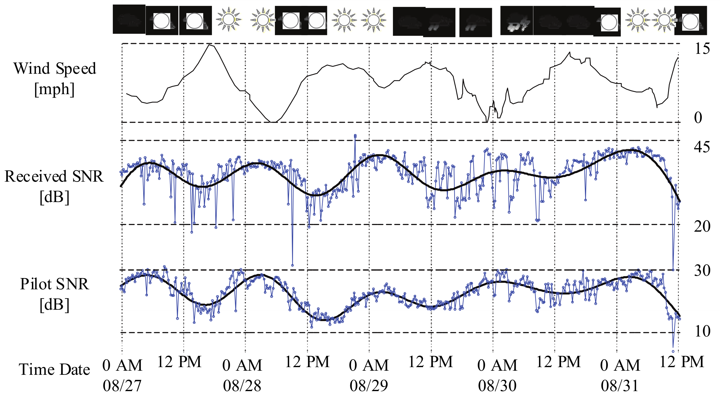
Figure 1.
Keweenaw Waterway experiment: Average signal-to-noise rates (SNR) at the receiver.
Figure 1.
Keweenaw Waterway experiment: Average signal-to-noise rates (SNR) at the receiver.
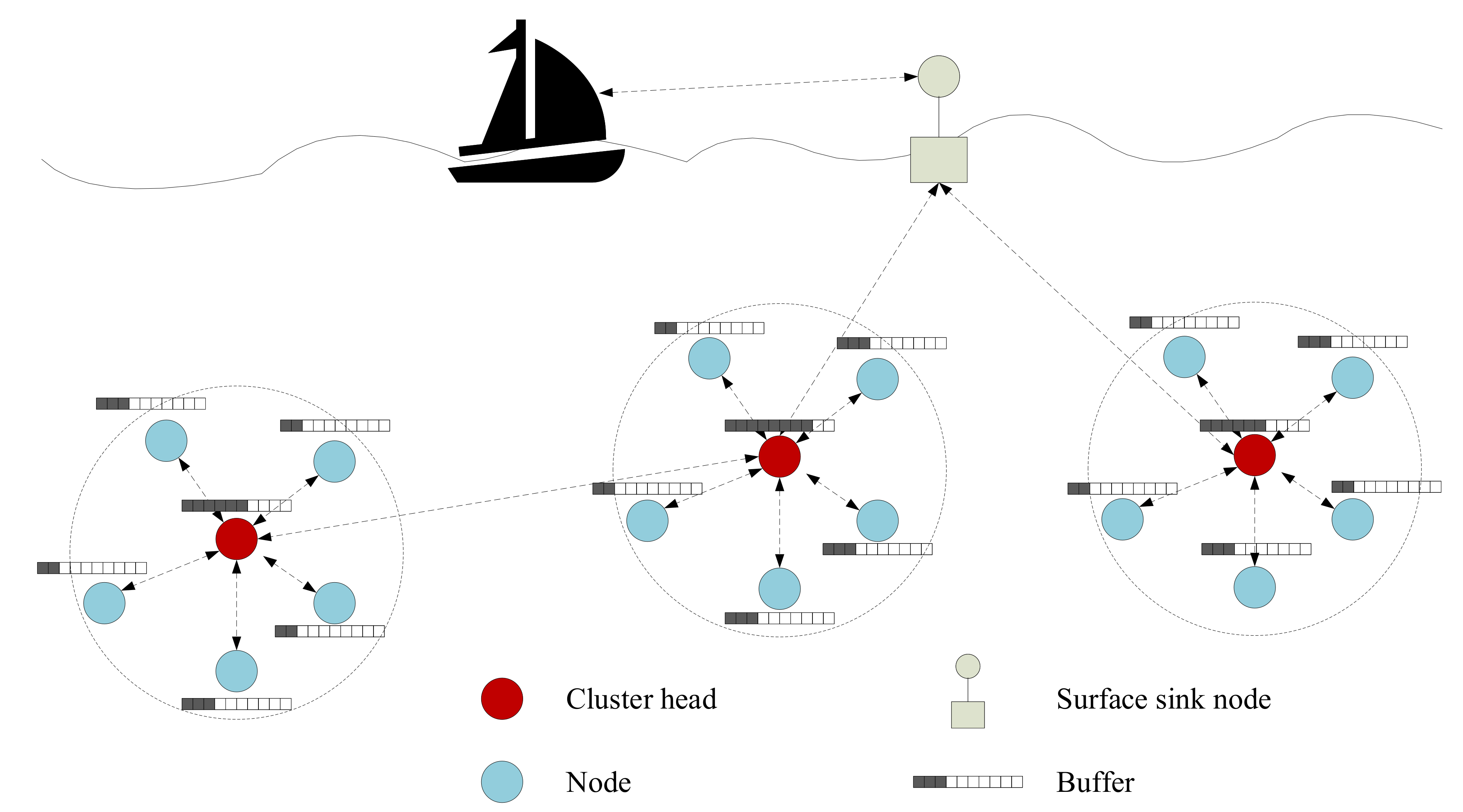
Figure 2.
Multi-hop clustered underwater acoustic sensor network.
Figure 2.
Multi-hop clustered underwater acoustic sensor network.
Figure 3.
Double-scale adaptive transmission mechanism.
Figure 3.
Double-scale adaptive transmission mechanism.
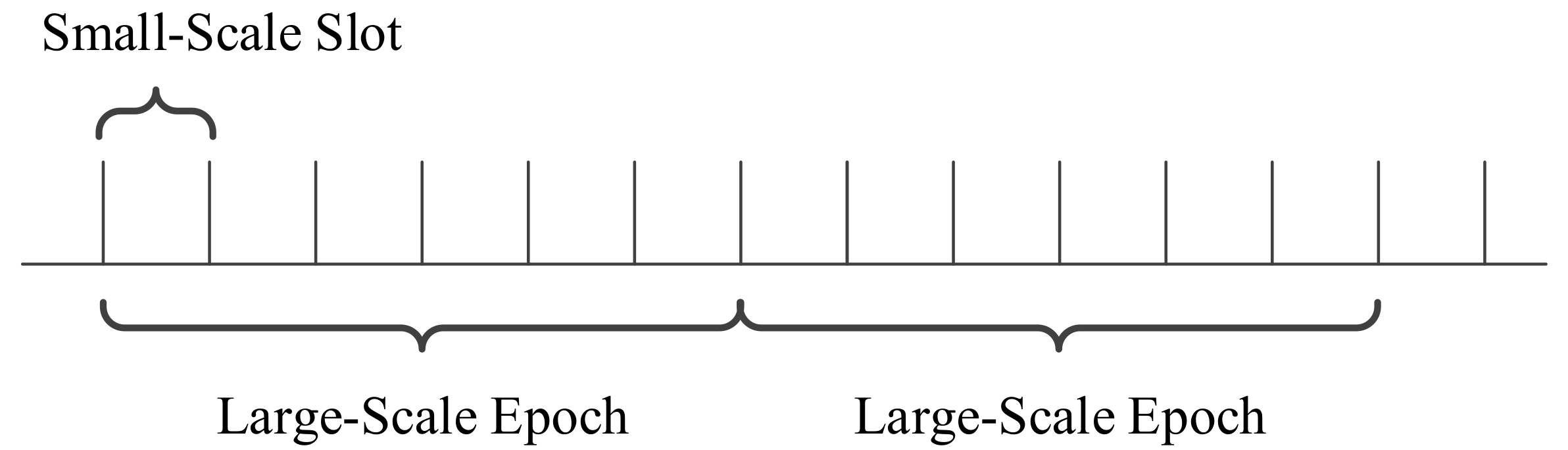
Figure 4.
Large-scale epoch and small-scale slot.
Figure 4.
Large-scale epoch and small-scale slot.
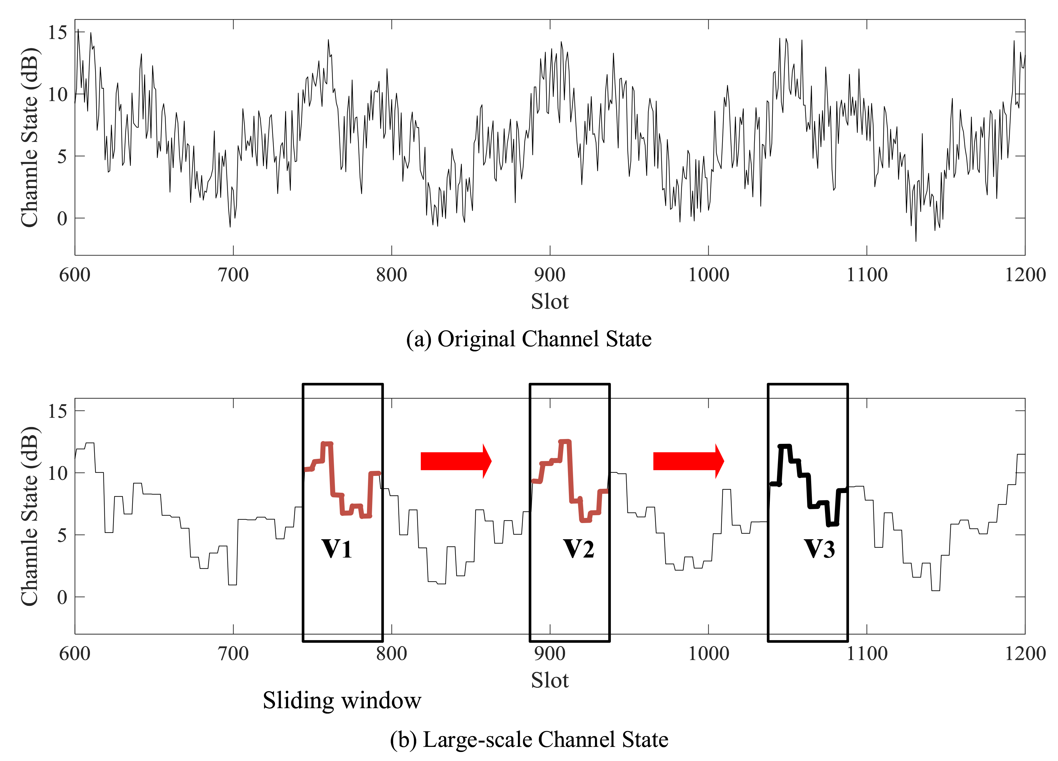
Figure 5.
Channel state and large-scale channel state prediction method. (a) Original channel state. (b) Large-scale channel state and diagram of k-nearest neighbor algorithm with sliding window. is the test vector. and are nearest neighbors chosen from training vectors.
Figure 5.
Channel state and large-scale channel state prediction method. (a) Original channel state. (b) Large-scale channel state and diagram of k-nearest neighbor algorithm with sliding window. is the test vector. and are nearest neighbors chosen from training vectors.
Figure 6.
Channel state series decomposition.
Figure 6.
Channel state series decomposition.
Figure 7.
Rearrangement process for a transmission modes chromosome.
Figure 7.
Rearrangement process for a transmission modes chromosome.
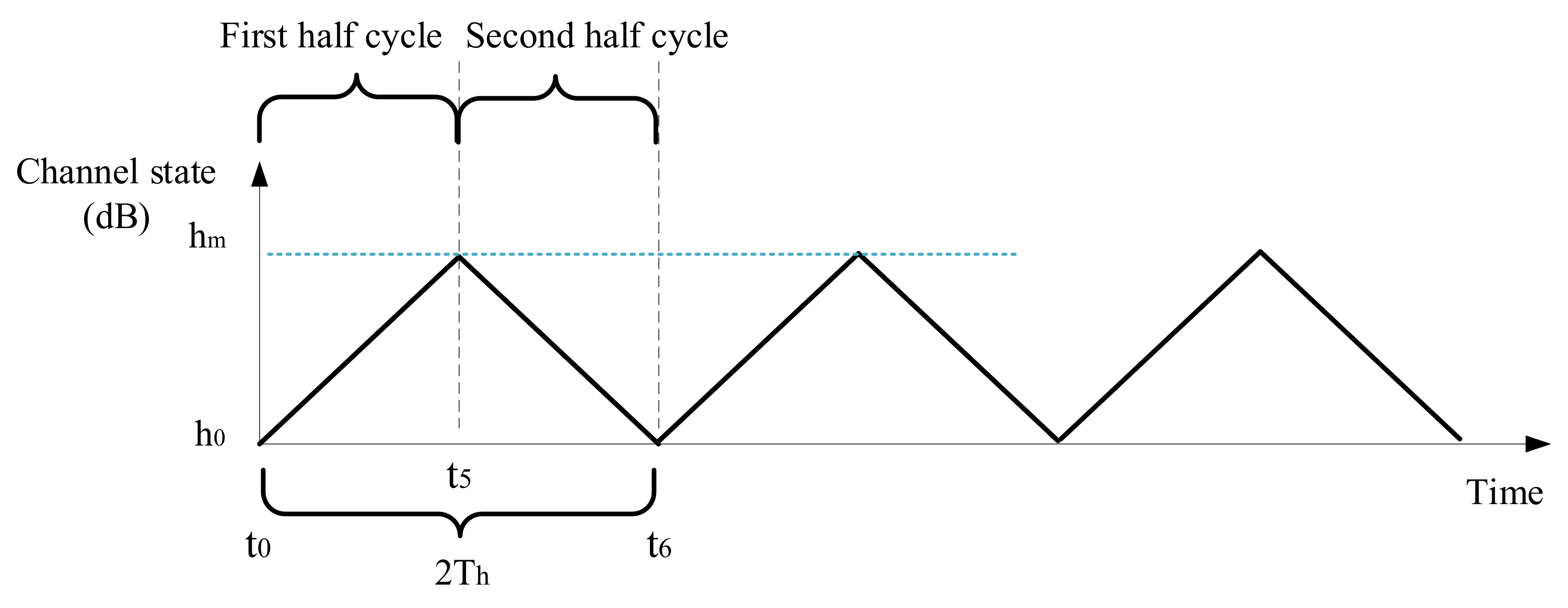
Figure 8.
A linearly varying channel state series.
Figure 8.
A linearly varying channel state series.
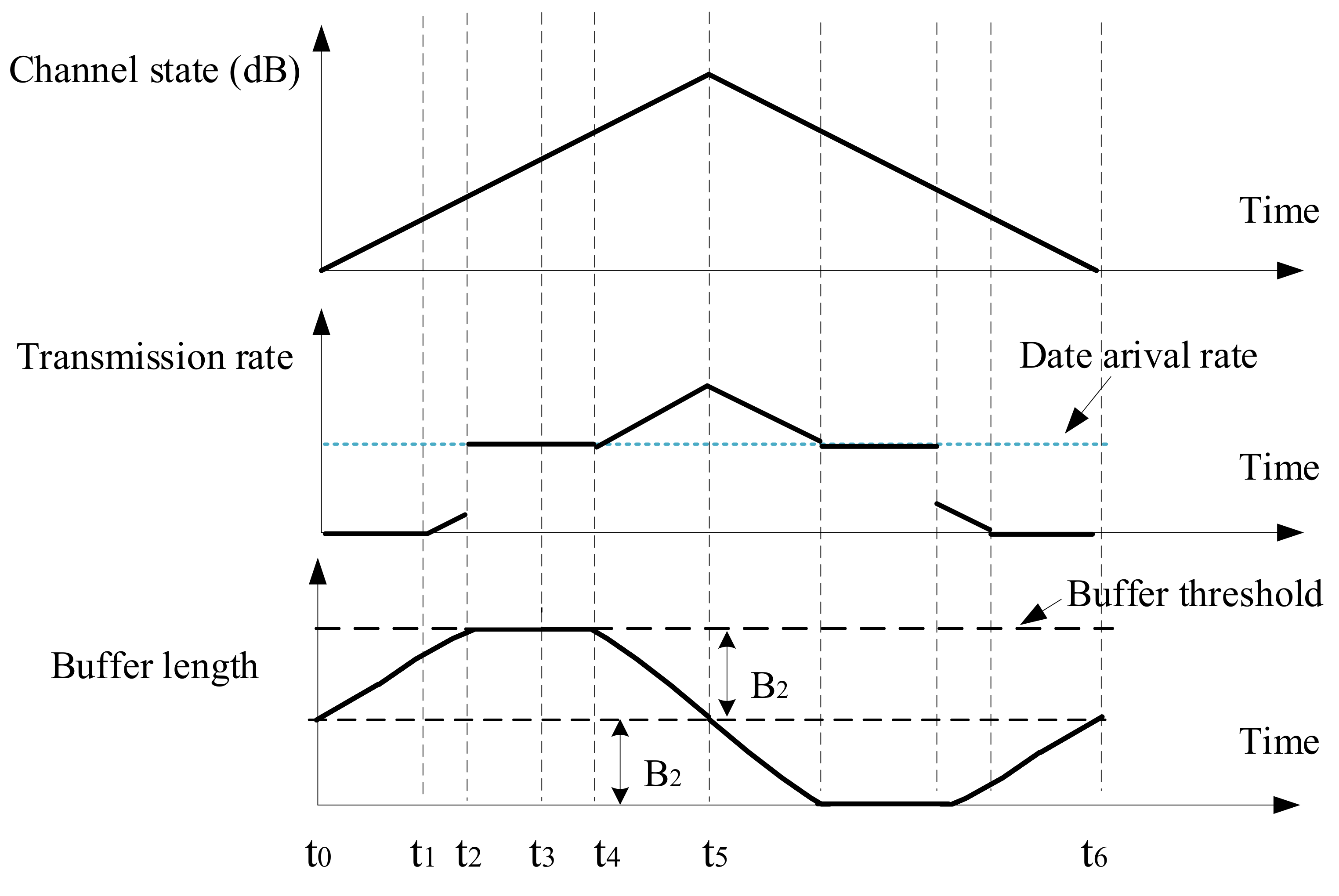
Figure 9.
Transmission action when buffer threshold is long enough (), for case 1.
Figure 9.
Transmission action when buffer threshold is long enough (), for case 1.
Figure 10.
Transmission action when , for case 2.
Figure 10.
Transmission action when , for case 2.
Figure 11.
Transmission action when , for case 3.
Figure 11.
Transmission action when , for case 3.
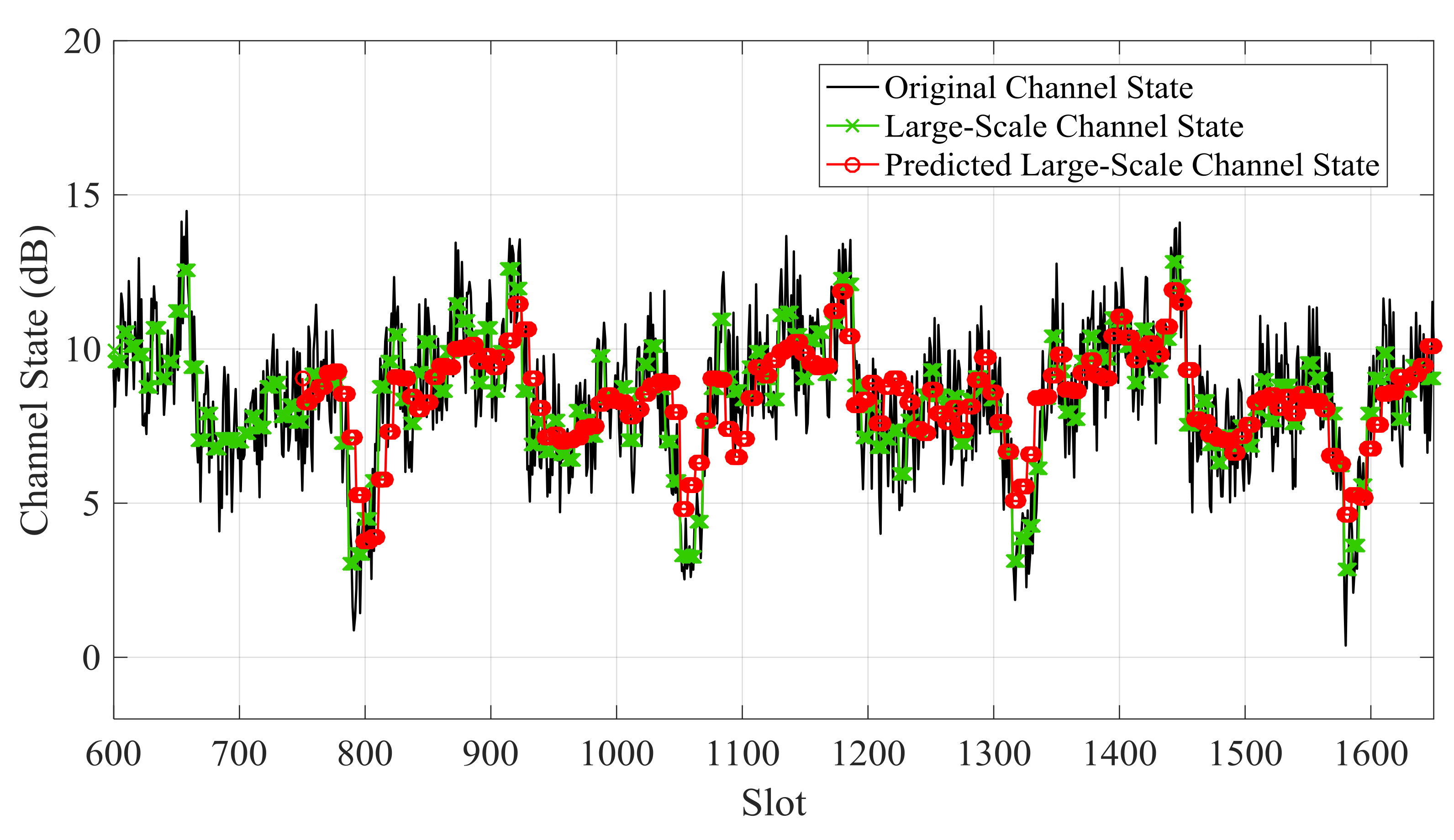
Figure 12.
Predicted large-scale channel state and real large-scale channel state of Data 1.
Figure 12.
Predicted large-scale channel state and real large-scale channel state of Data 1.
Figure 13.
Predicted large-scale channel state and real large-scale channel state of Data 2.
Figure 13.
Predicted large-scale channel state and real large-scale channel state of Data 2.
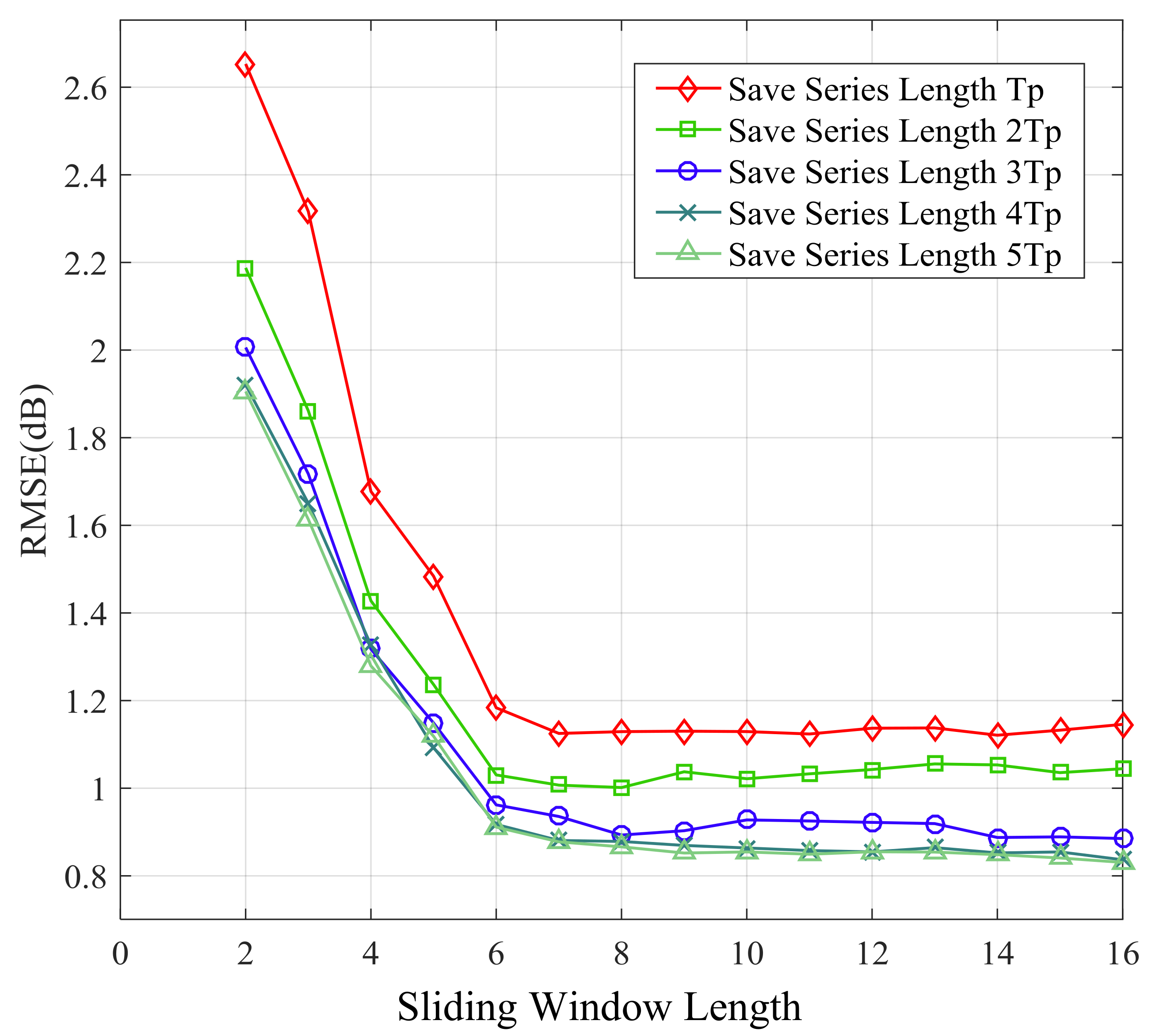
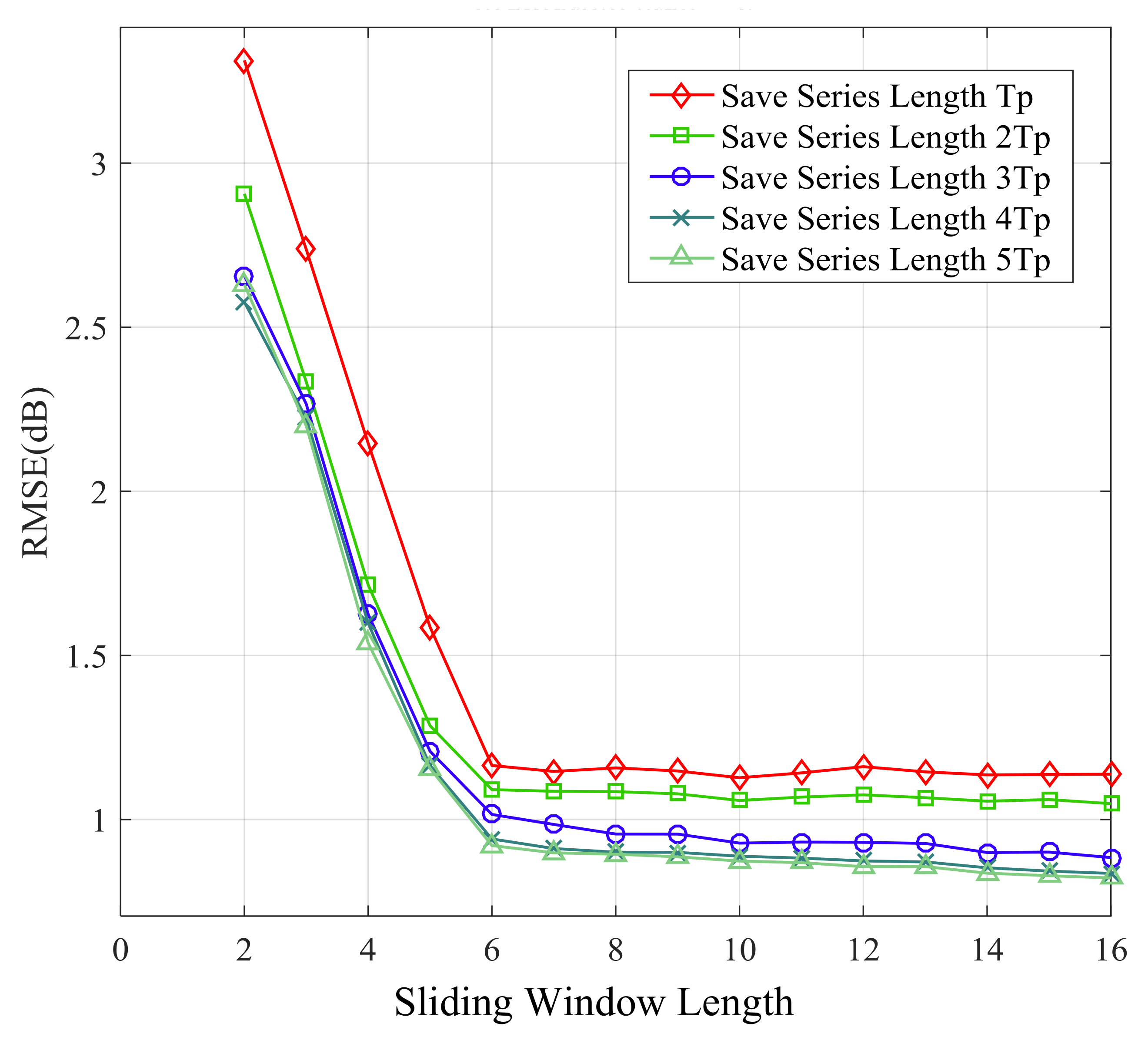
Figure 14.
Root mean square error (RMSE) of 1-step ahead prediction with different length of sliding window and stored series.
Figure 14.
Root mean square error (RMSE) of 1-step ahead prediction with different length of sliding window and stored series.
Figure 15.
RMSE of 5-step ahead prediction with different length of sliding window and stored series.
Figure 15.
RMSE of 5-step ahead prediction with different length of sliding window and stored series.
Figure 16.
RMSE of 15-step ahead prediction with different length of sliding window and stored series.
Figure 16.
RMSE of 15-step ahead prediction with different length of sliding window and stored series.
Figure 17.
RMSE of 25-step ahead prediction with different length of sliding window and stored series.
Figure 17.
RMSE of 25-step ahead prediction with different length of sliding window and stored series.
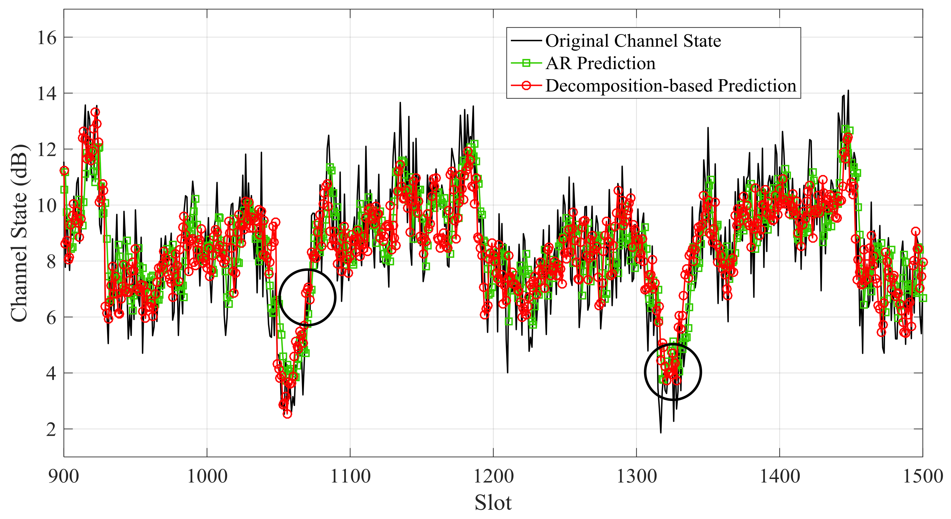
Figure 18.
Predicted small-scale channel state of Data 1 by the decomposition-based prediction model and auto-regressive (AR) prediction.
Figure 18.
Predicted small-scale channel state of Data 1 by the decomposition-based prediction model and auto-regressive (AR) prediction.
Figure 19.
Predicted small-scale channel state of Data 2 by the decomposition-based prediction model and AR prediction.
Figure 19.
Predicted small-scale channel state of Data 2 by the decomposition-based prediction model and AR prediction.
Figure 20.
RMSE of small-scale channel state prediction with different input vector length.
Figure 20.
RMSE of small-scale channel state prediction with different input vector length.
Figure 21.
Scheduled transmission mode according to predicted large-scale channel state for Data 1.
Figure 21.
Scheduled transmission mode according to predicted large-scale channel state for Data 1.
Figure 22.
Scheduled transmission mode according to predicted large-scale channel state for Data 2.
Figure 22.
Scheduled transmission mode according to predicted large-scale channel state for Data 2.
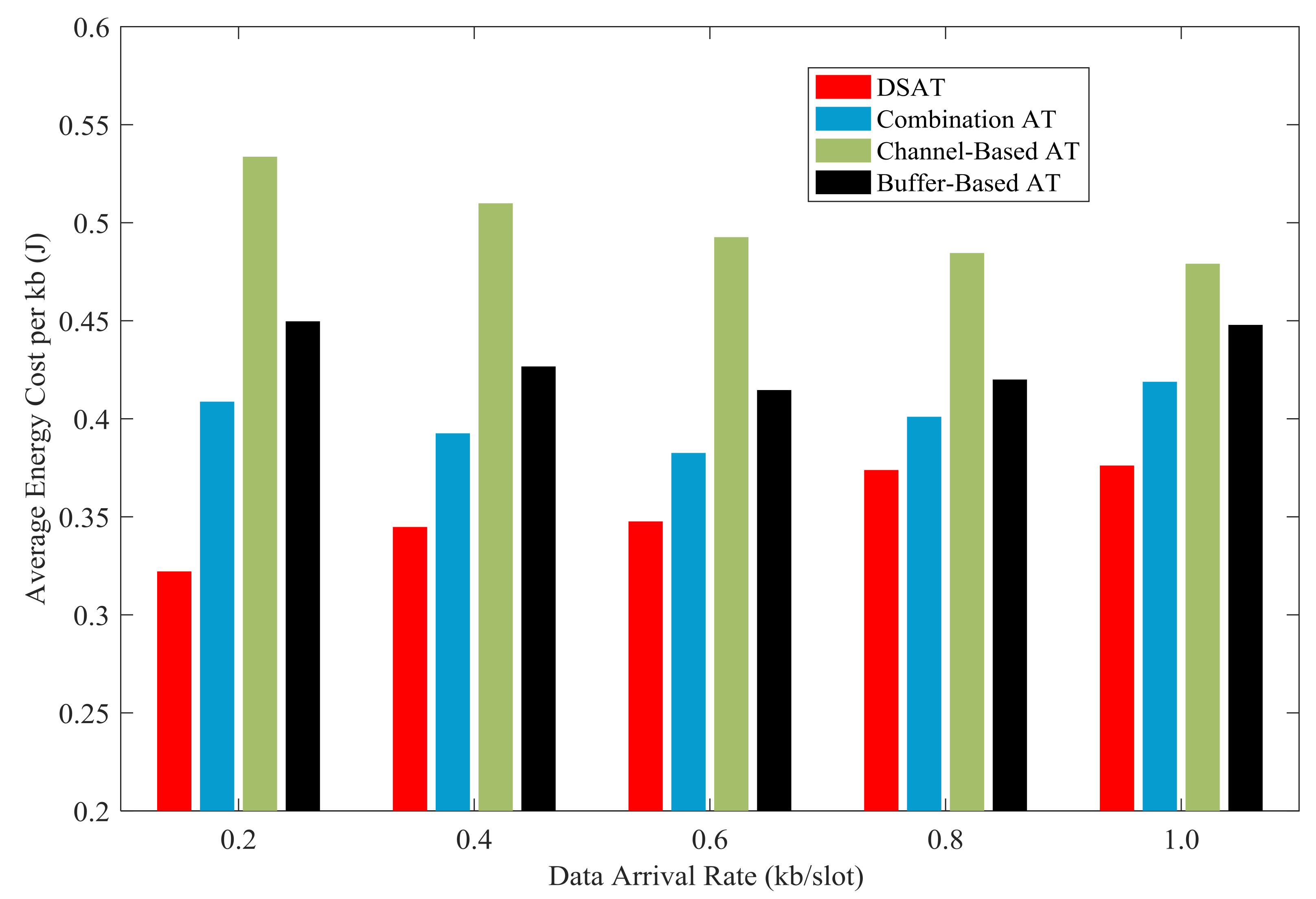
Figure 23.
Average energy cost per kb of for comparative strategies (Data 1).
Figure 23.
Average energy cost per kb of for comparative strategies (Data 1).
Figure 24.
Average energy cost per kb for comparative strategies (Data 2).
Figure 24.
Average energy cost per kb for comparative strategies (Data 2).
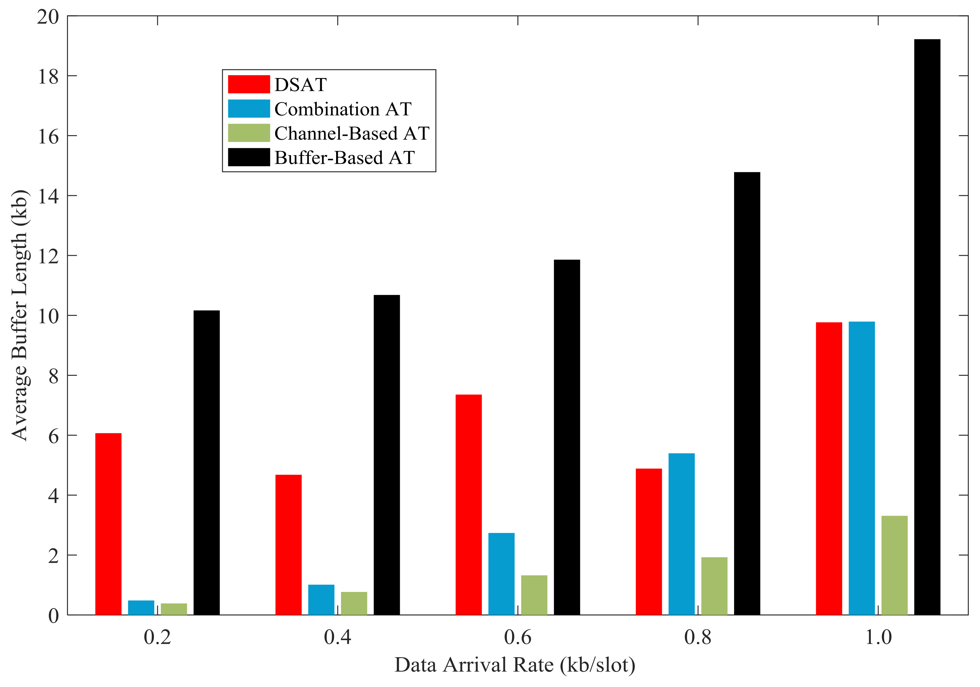
Figure 25.
Average buffer length for comparative strategies (Data 1).
Figure 25.
Average buffer length for comparative strategies (Data 1).
Figure 26.
Average buffer length for comparative strategies (Data 2).
Figure 26.
Average buffer length for comparative strategies (Data 2).
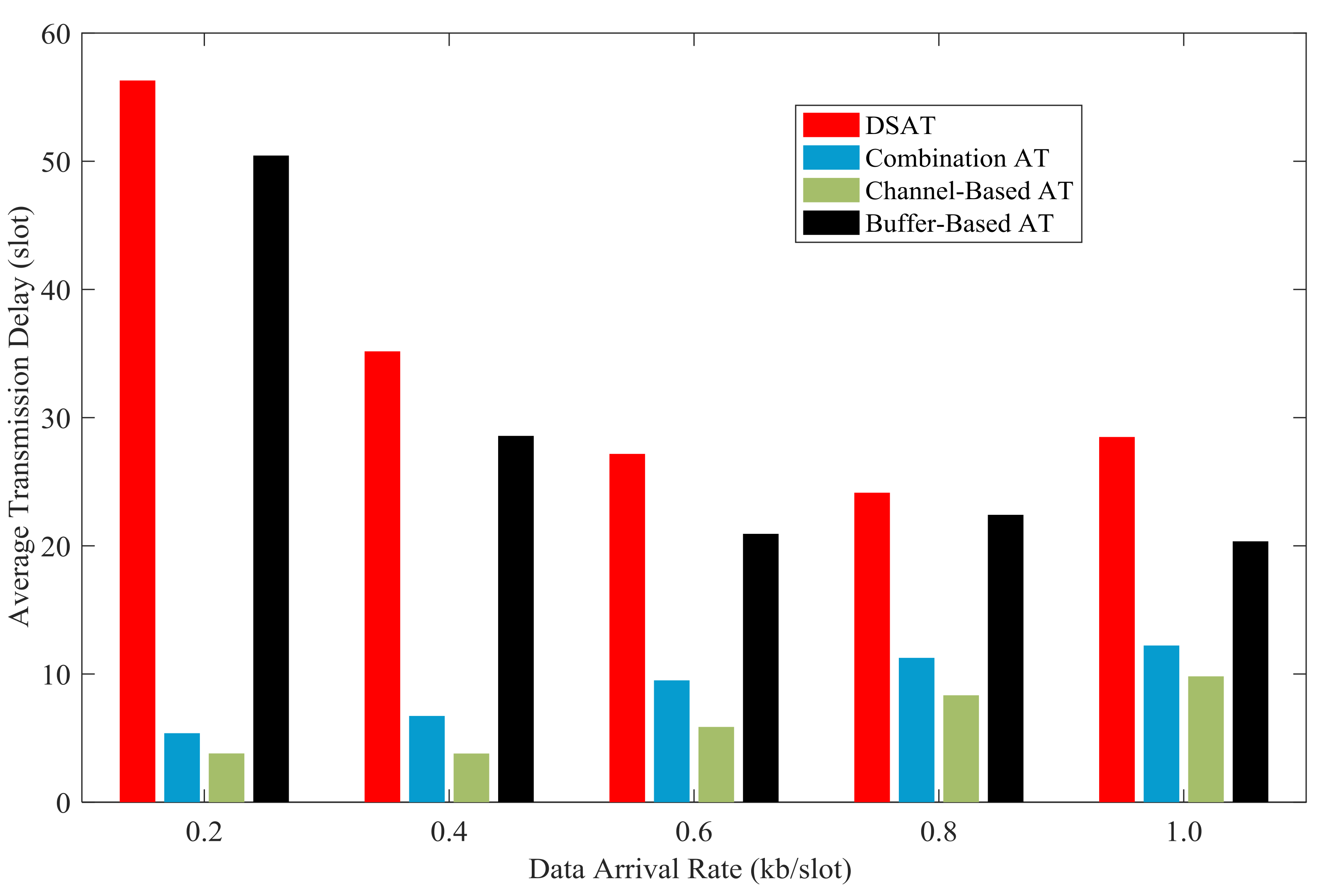
Figure 27.
Average transmission delay for comparative strategies (Data 1).
Figure 27.
Average transmission delay for comparative strategies (Data 1).
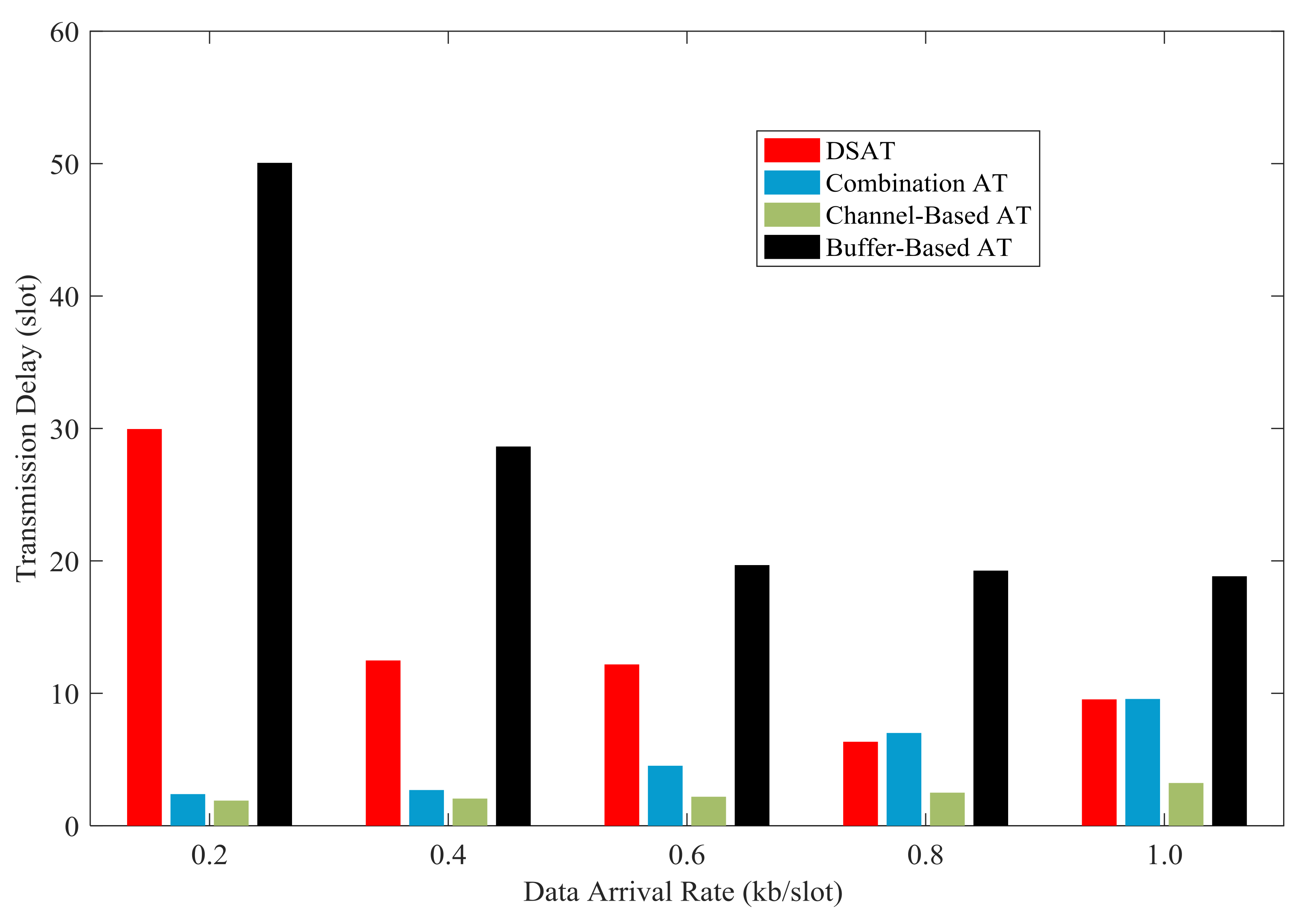
Figure 28.
Average transmission delay for comparative strategies (Data 2).
Figure 28.
Average transmission delay for comparative strategies (Data 2).
Figure 29.
Simulation results of the impact of buffer threshold and data arrival rate on the average energy cost.
Figure 29.
Simulation results of the impact of buffer threshold and data arrival rate on the average energy cost.
Figure 30.
Theoretical results of the impact of buffer threshold and data arrival rate on the average energy cost.
Figure 30.
Theoretical results of the impact of buffer threshold and data arrival rate on the average energy cost.
Figure 31.
Simulation results of the impact of buffer threshold and data arrival rate on the average buffer length.
Figure 31.
Simulation results of the impact of buffer threshold and data arrival rate on the average buffer length.
Figure 32.
Theoretical results of the impact of buffer threshold and data arrival rate on the average buffer length.
Figure 32.
Theoretical results of the impact of buffer threshold and data arrival rate on the average buffer length.
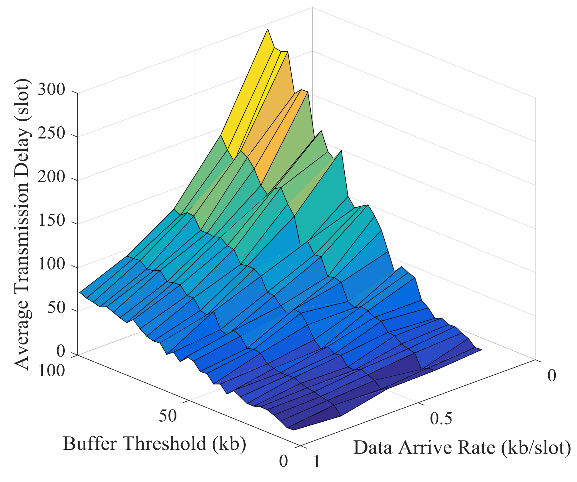
Figure 33.
Simulation results of the impact of buffer threshold and data arrival rate on the average transmission delay.
Figure 33.
Simulation results of the impact of buffer threshold and data arrival rate on the average transmission delay.
Figure 34.
Theoretical results of the impact of buffer threshold and data arrival rate on the average transmission delay.
Figure 34.
Theoretical results of the impact of buffer threshold and data arrival rate on the average transmission delay.
Table 1.
Simulation parameters.
Table 1.
Simulation parameters.
| Parameter | Value |
|---|
| Transmission distance | 1 km |
| Acoustic speed | 1500 m/s |
| Carrier frequency | 10 kHz |
| bandwidth | 5 kHz |
| Time slot | 2 s |
| Block size | 1000 symbols |
| Buffer Capacity | 100 kb |
Table 2.
Modulation and coding modes.
Table 2.
Modulation and coding modes.
| Transmission Mode | Modulation Methods | Coding Rate |
|---|
| Mode 0 | stop transmitting | |
| Mode 1 | BPSK | 1/2 |
| Mode 2 | QAM | 1/2 |
| Mode 3 | QAM | 3/4 |
| Mode 4 | 16QAM | 1/2 |
Table 3.
Comparative schemes.
Table 3.
Comparative schemes.
| Adaptive Schemes | Name | AMC Strategy | Channel Prediction Method |
|---|
| scheme 1 | DSAT | Energy-Efficient Transmission | Decomposition-based Prediction algorithm |
| scheme 2 | Combination AT | Combination AMC | AR Prediction algorithm |
| scheme 3 | Channel-Based AT | Channel-based AMC | AR Prediction algorithm |
| scheme 4 | Buffer-Based AT | Buffer-based AMC | AR Prediction algorithm |
Table 4.
Channel-based adaptive modulation and coding (AMC).
Table 4.
Channel-based adaptive modulation and coding (AMC).
| Channel State | Mode |
|---|
| h≤ | stop |
| < h≤ | Mode 1 |
| < h≤ | Mode 2 |
| < h≤ | Mode 3 |
| h > | Mode 4 |
Table 5.
Buffer-based AMC.
Table 5.
Buffer-based AMC.
| Buffer State | Mode |
|---|
| Buffer = 0 kb | stop |
| 0 kb < Buffer ≤ 5 kb | Mode 1 |
| 5 kb < Buffer ≤ 15 kb | Mode 2 |
| 15 kb < Buffer ≤ 25 kb | Mode 3 |
| Buffer > 25 kb | Mode 4 |
Table 6.
Combination AMC.
Table 6.
Combination AMC.
| Condition | Buffer ≤ 10 kb | 10 kb < Buffer ≤ 30 kb | Buffer > 30 kb |
|---|
| h > | Mode 2 | Mode 3 | Mode 4 |
| < h ≤ | Mode 1 | Mode 2 | Mode 3 |
| h≤ | stop | Mode 1 | Mode 2 |


