
In-Orbit Attitude Determination of the UVSQ-SAT CubeSat Using TRIAD and MEKF Methods

 , ,
, ,  ,
,
Abstract
:1. Introduction
2. UVSQ-SAT Attitude Determination Considerations
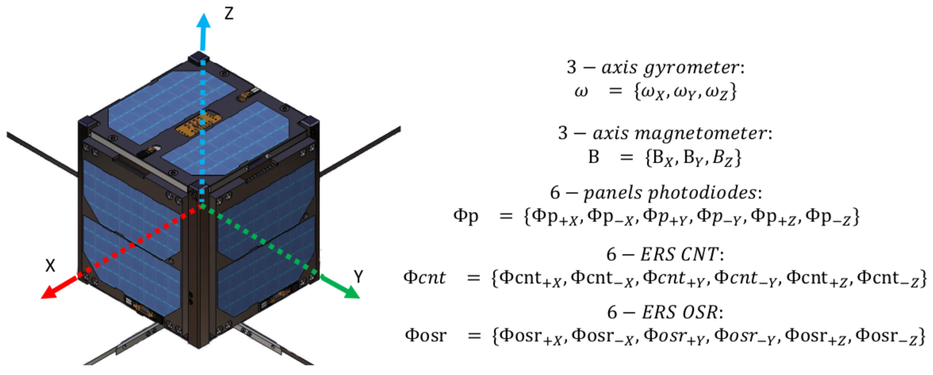
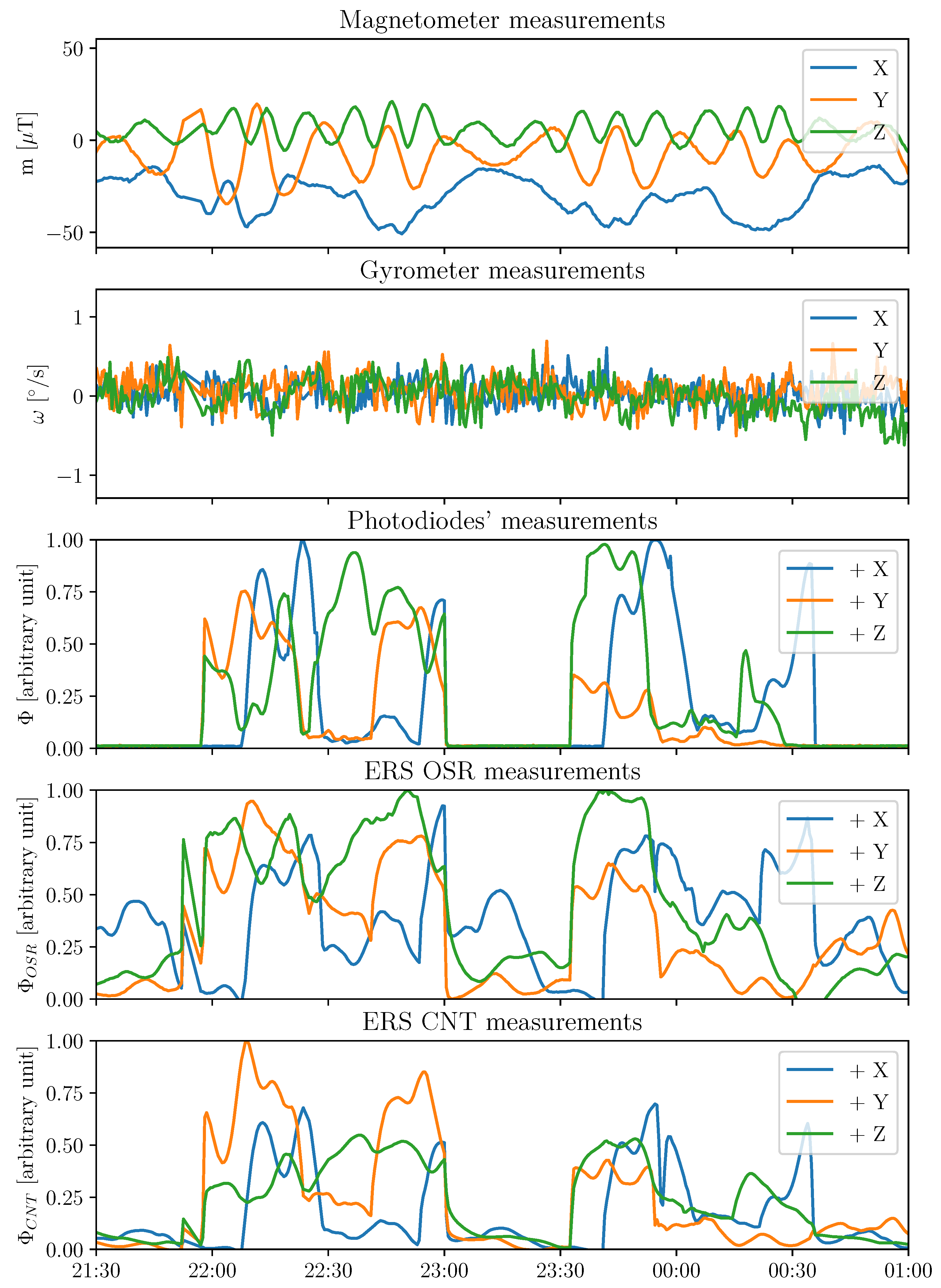
2.1. Sensors Description
- Three-axis angular velocities. The gyrometer measures the three-axis angular velocities in the sensor frame to the inertial reference frame (I), defined by , as the calibrated measurement.
- Three-axis magnetic field. The magnetometer measures the magnetic field along its three axes in the instrument’s reference frame defined by , as the calibrated measurement.
- Six photodiodes in the visible domain. They measure solar and outgoing shortwave radiations in the 400–1100 nm wavelength range. They are defined as the calibrated fluxes . They are used as a Sun sensor.
- Six Earth radiative sensors (ERS) sensors with an Optical Solar Reflector (OSR). They aim to measure radiation between 0.2 and 3 . They are defined as . Those sensors are used as an Earth sensor and aimed toward the nadir.
- Six ERS sensors with carbon nanotubes (CNT). Six sensors aim to measure total radiation between 0.2 and 100 m. They are defined as . They are used as Earth sensors.
2.2. Orbital Reference Frames and Attitude Representation
2.2.1. Orbital Reference Frames
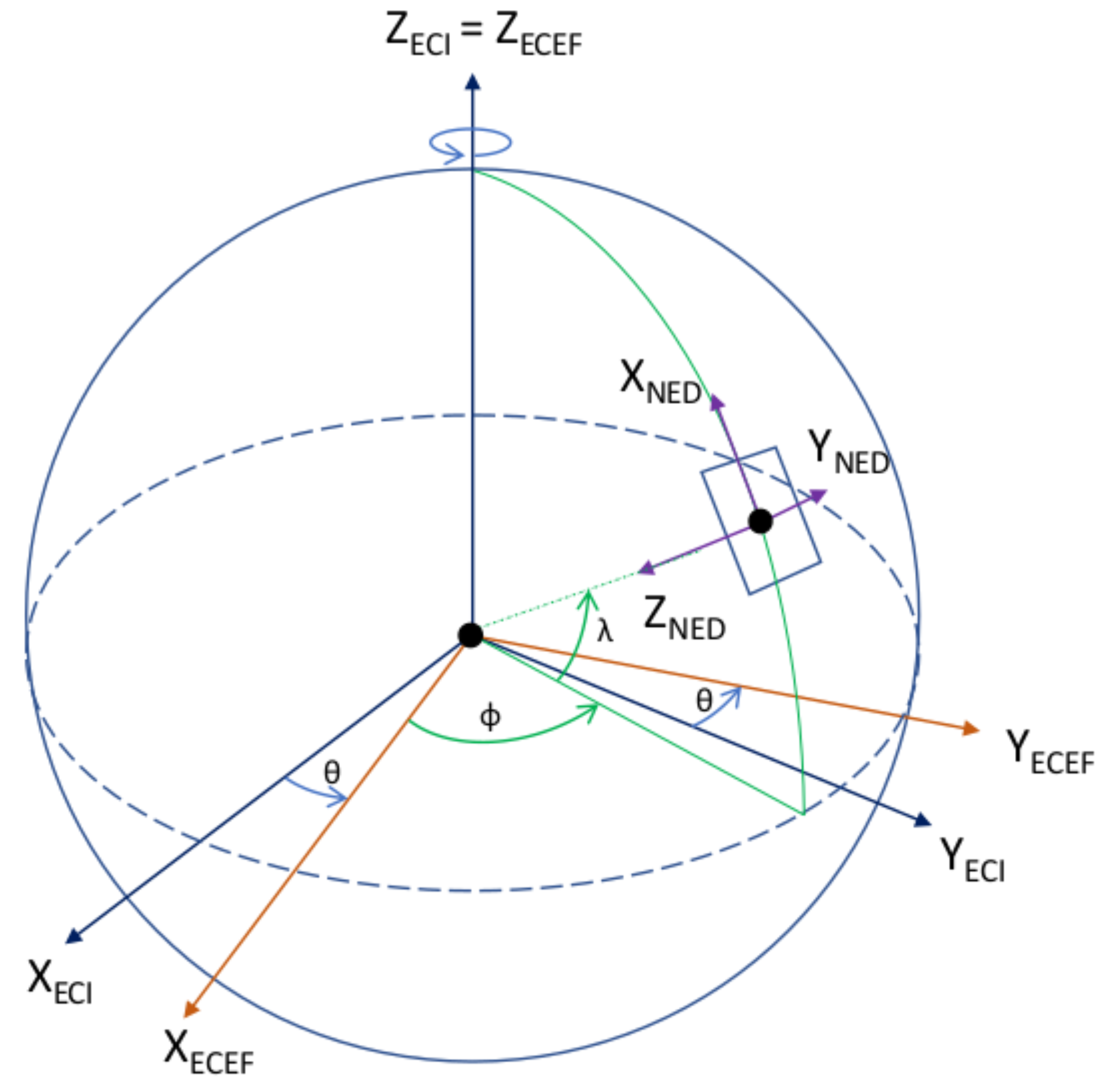
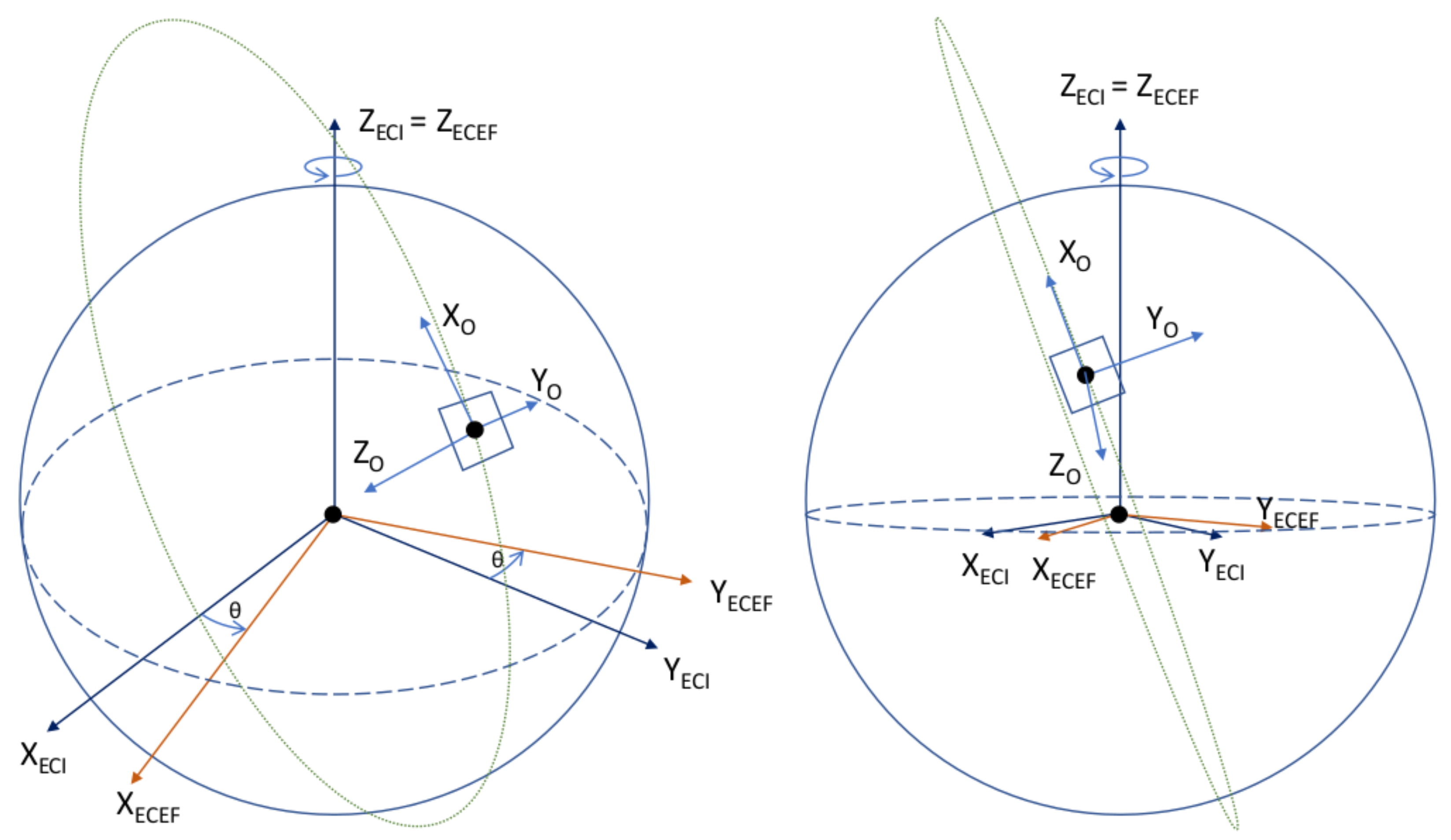
- Earth-centered inertial (ECI). The reference frame is defined in blue in Figure 3 with an origin at the Earth’s center of mass. The X-axis is defined as the vernal equinox axis at J2000, the intersection between the equatorial and the ecliptic planes. The Z-axis is defined as the Earth rotation axis at epoch J2000. Finally, the Y-axis is defined according to the previous directions to create an orthogonal basis.
- Earth-centered Earth-fixed (ECEF). The reference frame is defined in red in Figure 3 with its origin at the Earth’s center of mass. Its X-axis is defined at the intersection of the Greenwich prime meridian and the equator. Its Y-axis is the intersection of the equatorial plane and the 90 longitude. The Z-axis extends through the true north and south poles and coincides with the Earth’s rotation axis.
- North East Down (NED). Assuming a WGS84 ellipsoid model of the Earth, the NED, defined in purple in Figure 3, is a local reference frame that moves the body frame’s position in the ECEF. It is defined so that the X–Y plane is tangential to the surface of the ellipsoid at the given location in the ECEF. Given those conditions, the X-axis should point toward true North, the Z-axis toward the interior of the Earth, and the Y-axis will finalize the orthogonal basis.
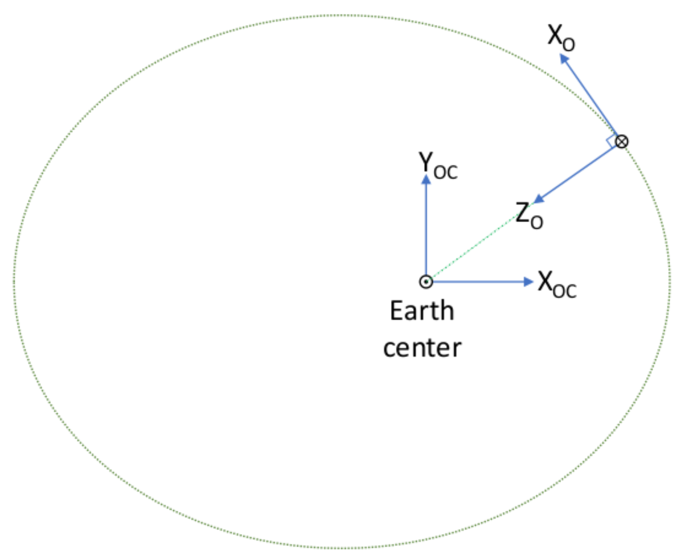
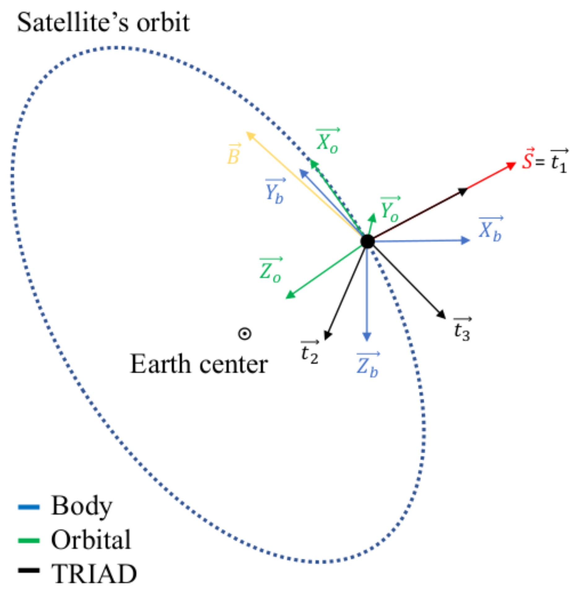
- Earth-centered orbit reference frame (OC). The reference frame is defined in blue in Figure 4 and Figure 5 and centered at the Earth’s center, with the X-axis towards the perigee, the Y-axis along the semi-minor axis, and the Z-axis perpendicular to the orbital plane to complete the right-hand system. From the previous reference frame, it is thus necessary to define a local reference frame that will follow the satellite in its center. This reference frame is chosen for its logic with respect to the satellite motion as well as the possibility of taking into account the orbital velocity in order to correct the gyrometer of this frame.
- Orbit reference frame (O). The reference frame is defined such that its origin is located at the center of the spacecraft. The origin rotates relative to the ECI with an angular velocity of . Its Z-axis points towards the center of the Earth. The X-axis is perpendicular to the previous axis in the spacecraft’s direction of motion. The Y-axis completes the right-hand system.
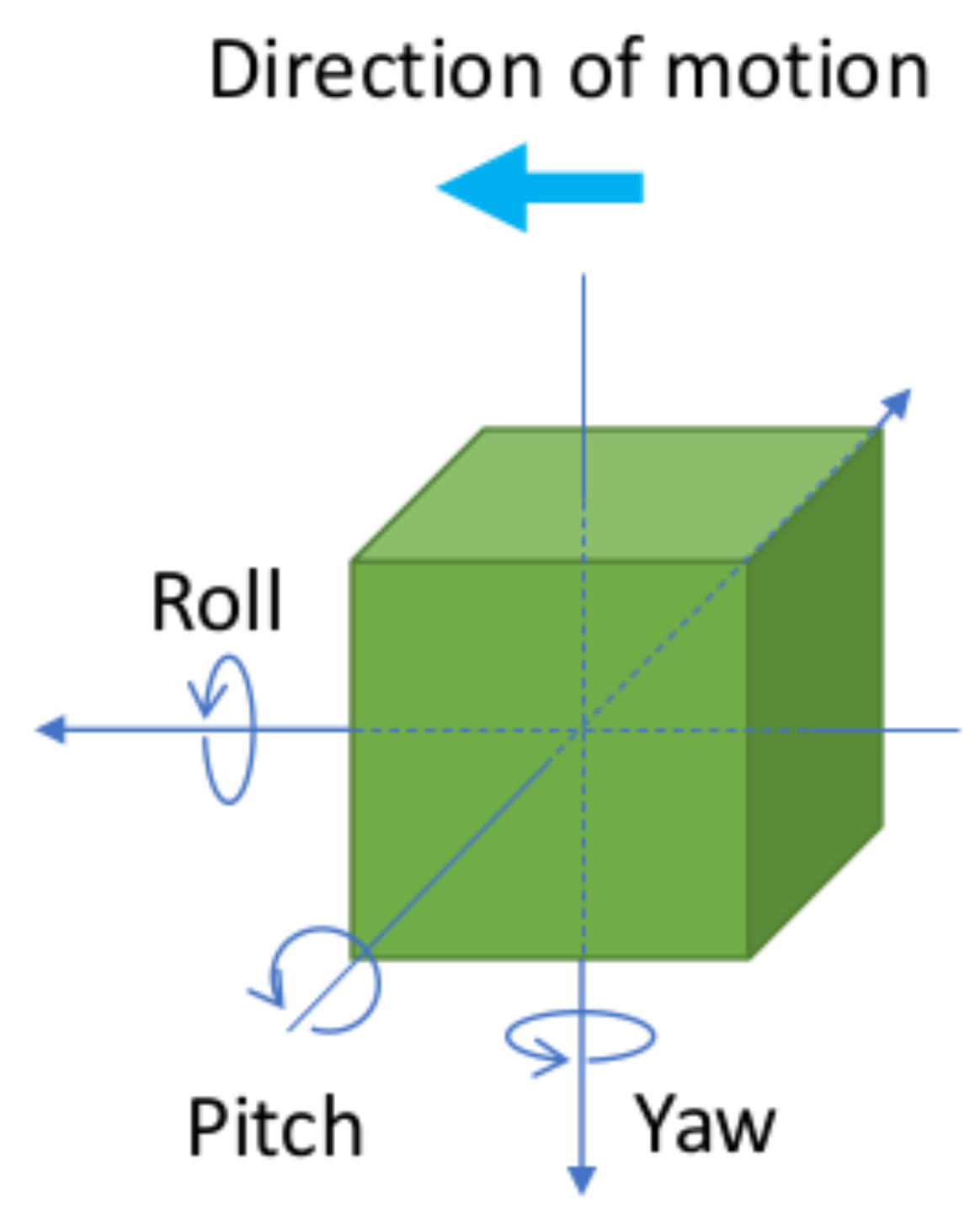
2.2.2. Attitude Representation
2.3. Theoretical Approach of the Method
3. Attitude Determination Methods
3.1. Tri-Axial Attitude Determination Method (TRIAD)
3.1.1. Formulation of the Method
3.1.2. Optimized TRIAD
3.2. Multiplicative Extended Kalman Method
3.2.1. Formulation
3.2.2. Initialization
3.2.3. Gain
3.2.4. Update
3.2.5. Propagation
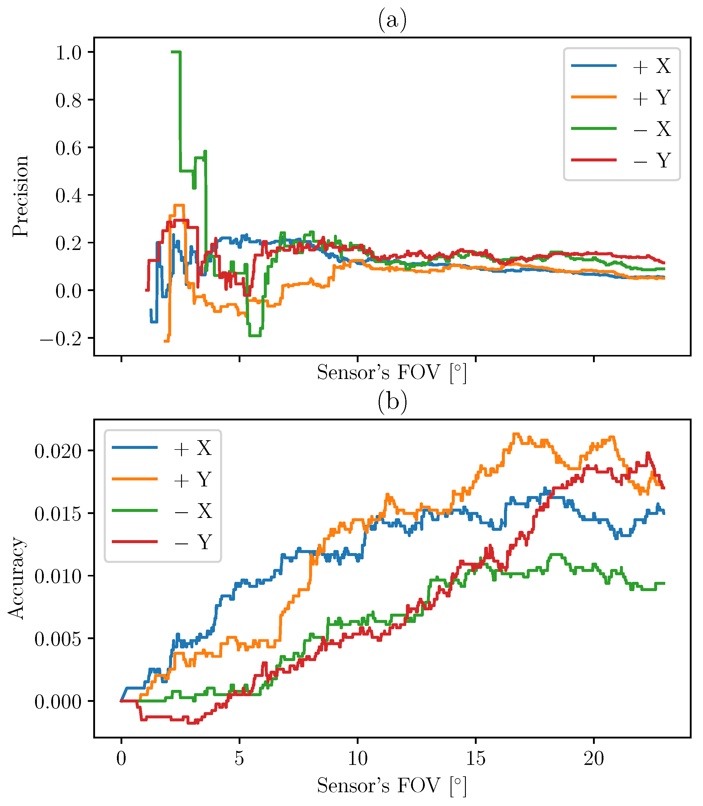
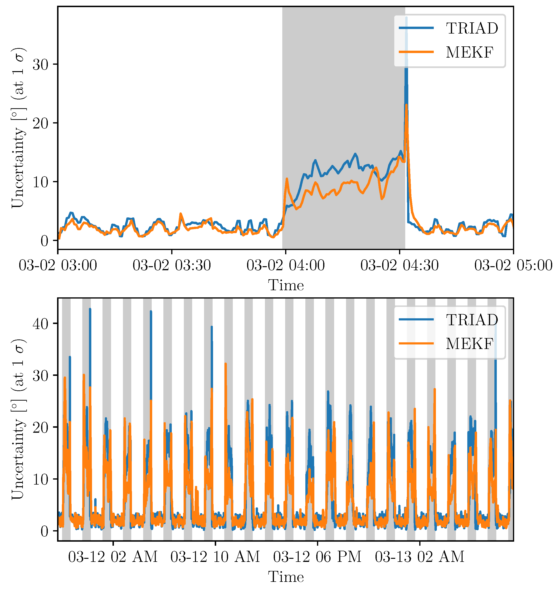
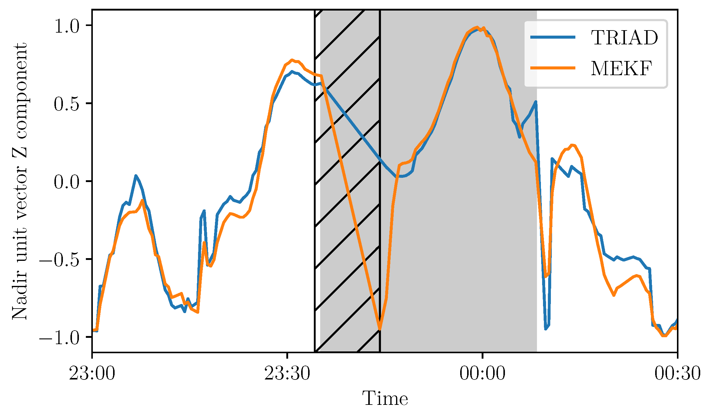
4. Results
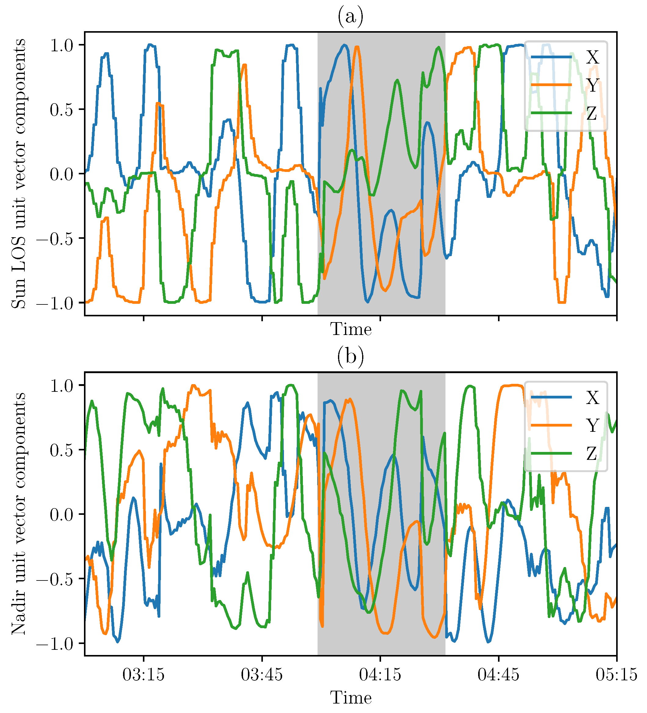
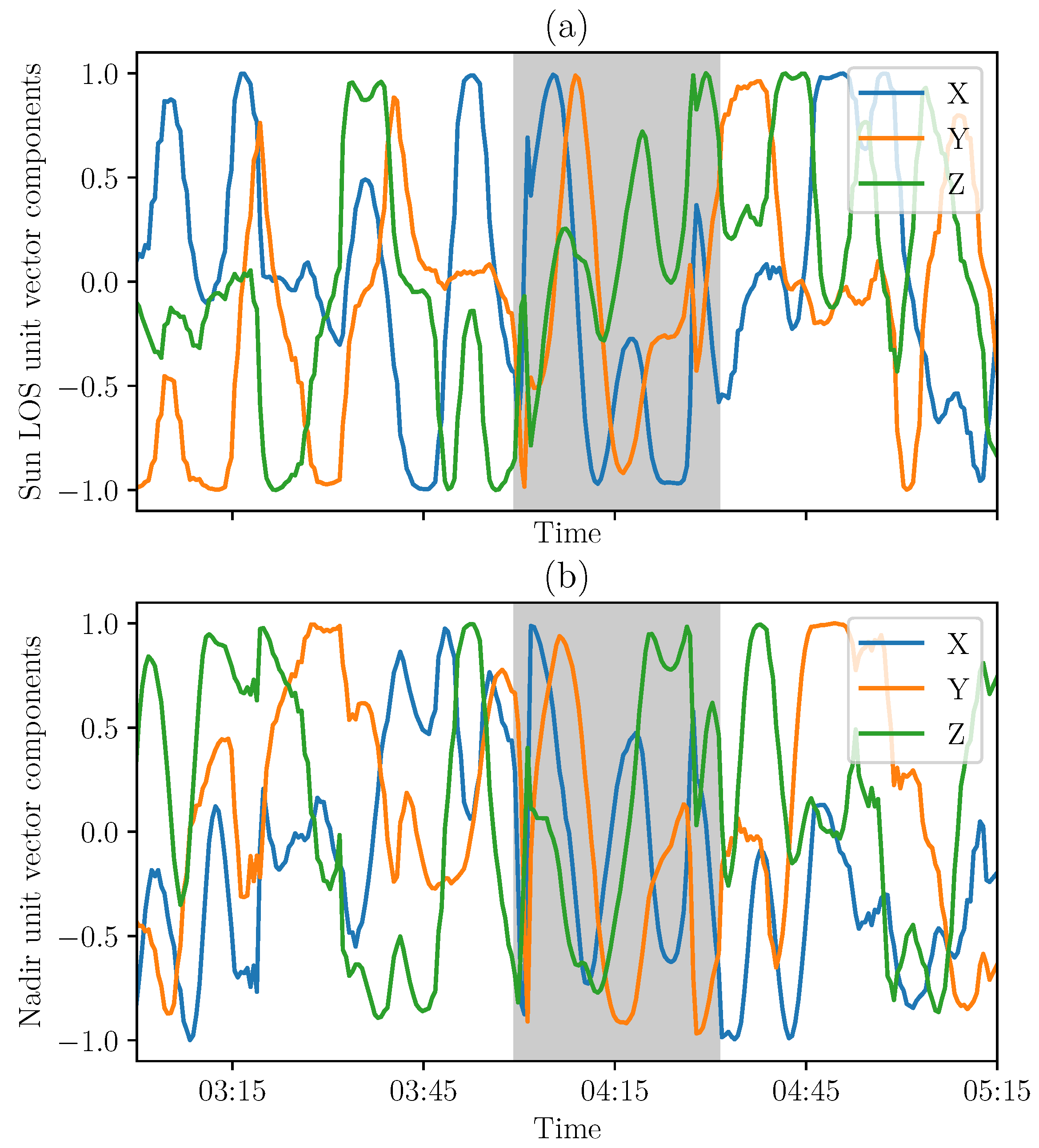
4.1. Results with TRIAD Method
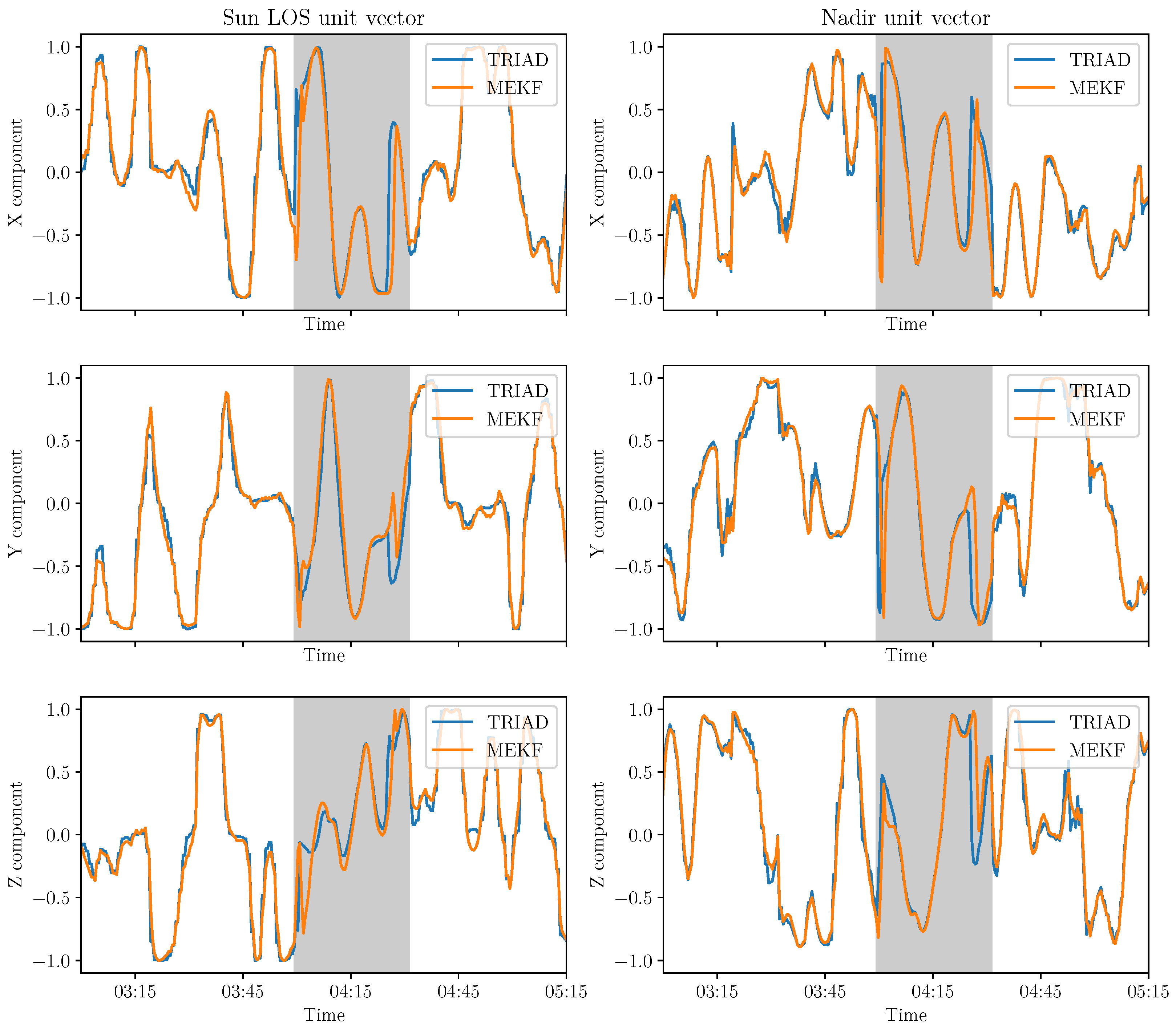
4.2. Results with MEKF Method
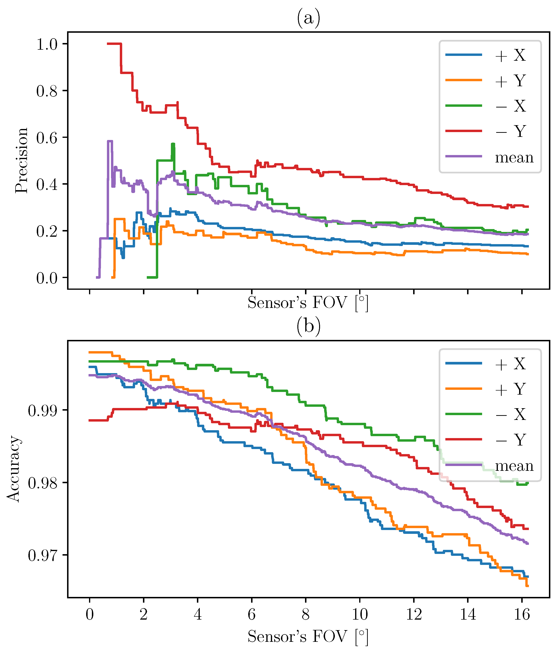
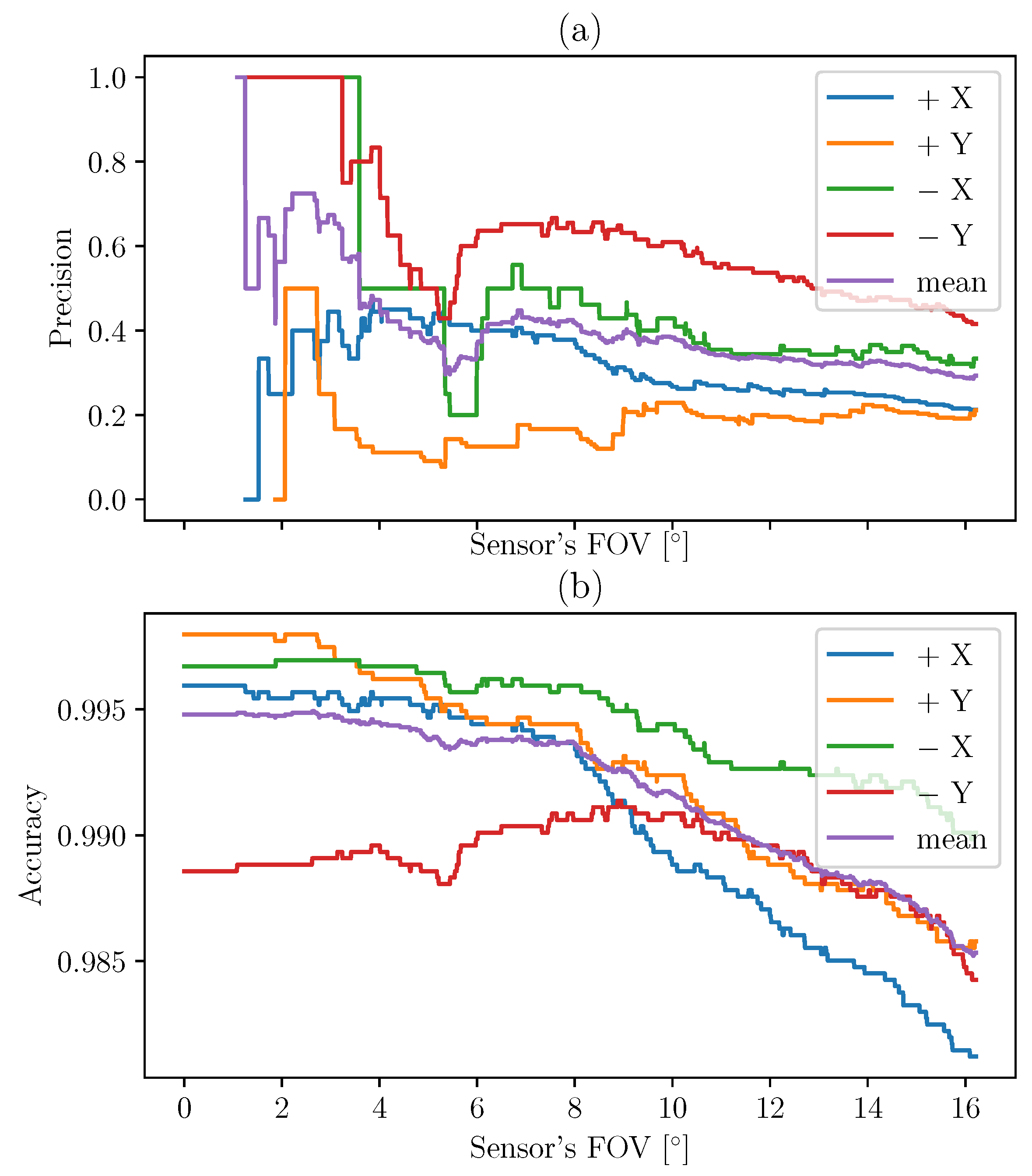
4.3. Discussion and Perspectives
5. Conclusions
Author Contributions
Funding
Institutional Review Board Statement
Informed Consent Statement
Data Availability Statement
Acknowledgments
Conflicts of Interest
References
- Meftah, M.; Damé, L.; Keckhut, P.; Bekki, S.; Sarkissian, A.; Hauchecorne, A.; Bertran, E.; Carta, J.P.; Rogers, D.; Abbaki, S.; et al. UVSQ-SAT, a pathfinder cubesat mission for observing essential climate variables. Remote Sens. 2020, 12, 92. [Google Scholar] [CrossRef] [Green Version]
- Meftah, M.; Boutéraon, T.; Dufour, C.; Hauchecorne, A.; Keckhut, P.; Finance, A.; Bekki, S.; Abbaki, S.; Bertran, E.; Damé, L.; et al. The UVSQ-SAT/INSPIRESat-5 CubeSat Mission: First In-Orbit Measurements of the Earth’s Outgoing Radiation. Remote Sens. 2021, 13, 1449. [Google Scholar] [CrossRef]
- Springmann, J.C.; Cutler, J.W. On-orbit Calibration of Photodiodes for Attitude Determination. J. Guid. Control. Dyn. 2014, 37, 1808–1823. [Google Scholar] [CrossRef] [Green Version]
- Psiaki, M.L.; Martel, F.; Pal, P.K. Three-axis attitude determination via Kalman filtering of magnetometer data. J. Guid. Control. Dyn. 1990, 13, 506–514. [Google Scholar] [CrossRef]
- Hashmall, J.A.; Radomski, M.; Sedlak, J. On-orbit calibration of satellite gyroscopes. In Proceedings of the Astrodynamics Specialist Conference, Minneapolis, MN, USA, 13–16 August 2000; pp. 339–349. [Google Scholar] [CrossRef] [Green Version]
- Pittelkau, M.E. Kalman Filtering for Spacecraft System Alignment Calibration. J. Guid. Control. Dyn. 2001, 24, 1187–1195. [Google Scholar] [CrossRef]
- Theil, S.; Appel, P.; Schleicher, A. Low Cost, Good Accuracy—Attitude Determination Using Magnetometer and Simple Sun Sensor. 2003. Available online: https://digitalcommons.usu.edu/smallsat/2003/All2003/81/ (accessed on 20 July 2021).
- Bhanderi, D.; Bak, T. Modeling Earth Albedo for Satellites in Earth Orbit. In Proceedings of the AIAA Guidance, Navigation, and Control Conference and Exhibit, San Francisco, CA, USA, 15–18 August 2005; Volume 8. [Google Scholar] [CrossRef] [Green Version]
- Ma, G.-F.; Jiang, X.-Y. Unscented Kalman Filter for Spacecraft Attitude Estimation and Calibration Using Magnetometer Measurements. In Proceedings of the 2005 International Conference on Machine Learning and Cybernetics, Guangzhou, China, 18–21 August 2005; Volume 1, pp. 506–511. [Google Scholar] [CrossRef]
- Côté, J.; De Lafontaine, J. Magnetic-only orbit and attitude estimation using the Square-Root Unscented Kalman Filter: Application to the PROBA-2 spacecraft. In AIAA Guidance, Navigation and Control Conference and Exhibit; AIAA: Reston, VA, USA, 2008; pp. 1–24. [Google Scholar] [CrossRef]
- Filipski, M.N.; Varatharajoo, R. Evaluation of a spacecraft attitude and rate estimation algorithm. Aircr. Eng. Aerosp. Technol. 2010, 82, 184–193. [Google Scholar] [CrossRef]
- Springmann, J.C.; Sloboda, A.J.; Klesh, A.T.; Bennett, M.W.; Cutler, J.W. The attitude determination system of the RAX satellite. Acta Astronaut. 2012, 75, 120–135. [Google Scholar] [CrossRef]
- Searcy, J.D.; Pernicka, H.J. Magnetometer-Only Attitude Determination Using Novel Two-Step Kalman Filter Approach. J. Guid. Control. Dyn. 2012, 35, 1693–1701. [Google Scholar] [CrossRef]
- Zeng, Z.; Zhang, S.; Xing, Y.; Cao, X. Robust Adaptive Filter for Small Satellite Attitude Estimation Based on Magnetometer and Gyro. Abstr. Appl. Anal. 2014, 2014, 159149. [Google Scholar] [CrossRef] [Green Version]
- Pham, M.D.; Low, K.S.; Goh, S.T.; Chen, S. Gain-scheduled extended Kalman filter for nanosatellite attitude determination system. IEEE Trans. Aerosp. Electron. Syst. 2015, 51, 1017–1028. [Google Scholar] [CrossRef]
- Kiani, M.; Pourtakdoust, S.H.; Sheikhy, A.A. Consistent calibration of magnetometers for nonlinear attitude determination. Meas. J. Int. Meas. Confed. 2015, 73, 180–190. [Google Scholar] [CrossRef]
- Koizumi, S.; Kikuya, Y.; Sasaki, K.; Masuda, Y.; Iwasaki, Y.; Watanabe, K. Development of Attitude Sensor using Deep Learning. In AIAA/USU Conference on Small Satellites; AIAA: Reston, VA, USA, 2018; pp. 1–8. [Google Scholar]
- Labibian, A.; Pourtakdoust, S.H.; Alikhani, A.; Fourati, H. Development of a radiation based heat model for satellite attitude determination. Aerosp. Sci. Technol. 2018, 82–83, 479–486. [Google Scholar] [CrossRef]
- Baroni, L. Attitude determination by unscented Kalman filter and solar panels as sun sensor. Eur. Phys. J. Spec. Top. 2020, 229, 1501–1506. [Google Scholar] [CrossRef]
- Kapás, K.; Bozóki, T.; Dálya, G.; Takátsy, J.; Mészáros, L.; Pál, A. Attitude Determination for Nano-Satellites—I. Spherical Projections for Large Field of View Infrasensors. Exp. Astron. 2021, 51, 1–13. [Google Scholar] [CrossRef]
- Mimasu, Y.; Narumi, T.; Van der Ha, J. Attitude Determination by Magnetometer and Gyros During Eclipse; AIAA: Reston, VA, USA, 2008. [Google Scholar] [CrossRef]
- Alken, P.; Thébault, E.; Beggan, C.D.; Amit, H.; Aubert, J.; Baerenzung, J.; Bondar, T.N.; Brown, W.J.; Califf, S.; Chambodut, A.; et al. International Geomagnetic Reference Field: The thirteenth generation. Earth Planets Space 2021, 73, 49. [Google Scholar] [CrossRef]
- Black, H.D. A passive system for determining the attitude of a satellite. AIAA J. 1964, 2, 1350–1351. [Google Scholar] [CrossRef]
- Markley, F.L.; Mortari, D. How to estimate attitude from vector observations. Adv. Astronaut. Sci. 2000, 103, 1979–1996. [Google Scholar]
- Bar-Itzhack, I.Y.; Harman, R.R. Optimized TRIAD Algorithm for Attitude Determination. J. Guid. Control. Dyn. 1997, 20, 208–211. [Google Scholar] [CrossRef] [Green Version]
- Bar-itzhack, I.Y.; Meyer, J. On the Convergence of Iterative Orthogonalization Processes. IEEE Trans. Aerosp. Electron. Syst. 1976, AES-12, 146–151. [Google Scholar] [CrossRef]
- Kalman, R.E. A New Approach to Linear Filtering and Prediction Problems. Trans. ASME-Basic Eng. 1960, 82, 35–45. [Google Scholar] [CrossRef] [Green Version]
- Kalman, R.E.; Bucy, R.S. New Results in Linear Filtering and Prediction Theory. J. Basic Eng. 1961, 83, 95–108. [Google Scholar] [CrossRef]
- Markley, F.L.; Crassidis, J.L. Static Attitude Determination Methods. In Fundamentals of Spacecraft Attitude Determination and Control; Springer: New York, NY, USA, 2014; pp. 183–233. [Google Scholar] [CrossRef]
- Lefferts, E.J.; Markley, F.L.; Shuster, M.D. Kalman Filtering for Spacecraft Attitude Estimation. J. Guid. Control. Dyn. 1982, 5, 417–429. [Google Scholar] [CrossRef]
- Finance, A.; Meftah, M.; Dufour, C.; Boutéraon, T.; Bekki, S.; Hauchecorne, A.; Keckhut, P.; Sarkissian, A.; Damé, L.; Mangin, A. A New Method Based on a Multilayer Perceptron Network to Determine In-Orbit Satellite Attitude for Spacecrafts without active ADCS like UVSQ-SAT. Remote Sens. 2021, 13, 1185. [Google Scholar] [CrossRef]


| Reference | Method (Instruments) | Goal | Results/Remarks |
|---|---|---|---|
| [4] | Simulation | Attitude determination (AD) based solely on magnetometer | Converges from initial attitude errors of maximum 60 and with an attitude accuracy of 1 (1) or better |
| [5] | Observation (Rossi X-ray Timing Explorer satellite calibration maneuvers, Terra and Wide-Field Infrared Explorer mission, Upper Atmosphere Research Satellite (UARS)) | On-orbit calibration of satellite gyroscopes | Methods comparison (attitude accuracy below 1). The Delta-bias algorithm gives slightly less accurate results than the Davenport and BICal algorithms |
| [6] | Simulation | Absolute alignment calibration of a system comprising two star trackers, an inertial sensor assembly (ISA) of three fiber-optic gyros, and an imaging instrument based on Alignment Kalman Filter (AKF) | AKF is effective to estimate absolute misalignments and gyro calibration parameters |
| [7] | Simulation | AD using an Extended Kalman Filter (EKF), which applies the albedo model with a magnetometer and sun sensor | Attitude accuracy below 1 |
| [8] | Simulation and Observation (Total Ozone Mapping Spectrometer (TOMS)) | Modeling the albedo for Sun/Earth sensor used in attitude determination | Albedo compensation in attitude estimation, improves the maximum error from 9.9 to 1.9 |
| [9] | Simulation | AD using Unscented Kalman Filter (UKF) based only on magnetometer | The attitude estimation accuracies are below 0.5 after convergence |
| [10] | Simulation (PROBA-2 Spacecraft scenarios) | Navigation system for magnetic-only orbit and attitude estimation using the square-root Unscented filter (MAGSURF) | RSS attitude error of less than 1.4 and a time of convergence of less than 2 orbits |
| [11] | Simulation | Attitude and rate estimation algorithm using EKF based only on geomagnetic field data | Filter converges within the +/−8 range for any initial attitude error |
| [12] | Simulation (Radio Aurora Explorer satellites (3U CubeSat)) | AD based on gyros, magnetometers, coarse sun sensors, and an EKF | In the sun, the angular uncertainty is between 2 and 3, and in eclipse, the uncertainty increases to between 7 and 8 |
| [13] | Simulation | AD using two-step EKF based on a magnetometer only | Attitude accuracies of less than 1 |
| [3] | Observation (Radio Aurora Explorer satellites (3U CubeSat)) | Photodiodes calibration and AD from EKF/UKF with albedo model based on the calibrated photodiodes, three-axis magnetometer and gyrometer | Angular improvement of 10 in sun vector from the photodiodes, and below 1 accuracy on the attitude determination |
| [14] | Simulation | AD via a robust Adaptive Kalman Filter based on magnetometer and gyro measurement | Precision of traditional EKF is about 0.2, and the maximum estimate error of the robust adaptive filter is 0.1 |
| [15] | Simulation and Observation (experimental data with on-ground nano-satellite) | Gain-scheduled EKF (GSEKF) to reduce the computational requirement in the nanosatellite attitude determination process | Attitude accuracy below 0.2 during the entire orbital period. Computation time could be reduced by 86.29% and 89.45% |
| [16] | Simulation | Magnetometer calibration with Hyper least square (HyperLS) estimator for ellipsoid fitting, then utilized for attitude determination via non-linear colored noise filters of EKF, simplex UKF and cubature Kalman filter | Attitude accuracy below 1 for simplex UKF |
| [17] | Observation (images taken from International Space Station (ISS)) | AD utilizing color earth images taken with visible light camera | Attitude accuracy is about few degrees or less |
| [18] | Simulation | Heat attitude model for satellite attitude determination | Attitude accuracy between 0.2 to 5 |
| [19] | Simulation | AD method based on an UKF, using a gyrometer, a magnetometer and solar panels as a sun sensor | The UKF has shown precision in Euler angles of about 1.1, which is better than for EKF. UKF has a considerably longer processing time compared to EKF |
| [20] | Simulation and Observation (experimentation on-ground set up) | Thermal imaging sensors to determine attitude of the Sun and the horizon by employing a homogeneous array of such detectors | Angular accuracy below 1 |
| Definition | Attitude Determination | ||
|---|---|---|---|
| Facing the Sun | Not facing the Sun | ||
| UVS | Facing the Sun | True Positive (TP) | False Negative (FN) |
| Not Facing the Sun | False Positive (FP) | True Negative (TN) | |
Publisher’s Note: MDPI stays neutral with regard to jurisdictional claims in published maps and institutional affiliations. |
© 2021 by the authors. Licensee MDPI, Basel, Switzerland. This article is an open access article distributed under the terms and conditions of the Creative Commons Attribution (CC BY) license (https://creativecommons.org/licenses/by/4.0/).
Share and Cite
Finance, A.; Dufour, C.; Boutéraon, T.; Sarkissian, A.; Mangin, A.; Keckhut, P.; Meftah, M. In-Orbit Attitude Determination of the UVSQ-SAT CubeSat Using TRIAD and MEKF Methods. Sensors 2021, 21, 7361. https://doi.org/10.3390/s21217361
Finance A, Dufour C, Boutéraon T, Sarkissian A, Mangin A, Keckhut P, Meftah M. In-Orbit Attitude Determination of the UVSQ-SAT CubeSat Using TRIAD and MEKF Methods. Sensors. 2021; 21(21):7361. https://doi.org/10.3390/s21217361
Chicago/Turabian StyleFinance, Adrien, Christophe Dufour, Thomas Boutéraon, Alain Sarkissian, Antoine Mangin, Philippe Keckhut, and Mustapha Meftah. 2021. "In-Orbit Attitude Determination of the UVSQ-SAT CubeSat Using TRIAD and MEKF Methods" Sensors 21, no. 21: 7361. https://doi.org/10.3390/s21217361