
Optimal Training Configurations of a CNN-LSTM-Based Tracker for a Fall Frame Detection System


Abstract
:1. Introduction
- Modification of state-of-the-art CNN architecture, namely VGG-M architecture, to produce a more compact architecture that is suitable for single object tracking applications;
- The strategy in maintaining the multiple-model object appearance of SmartConvFall that is used to handle model drift and noisy updates;
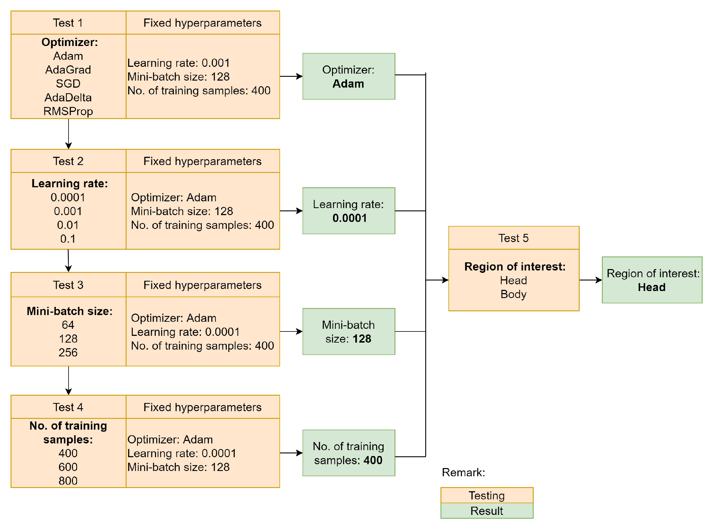
- Extensive comparison of training configurations that cover the selection of the optimizer, learning rate, mini-batch size, number of training samples, and region of interest schemes to obtain the best object appearance model for SmartConvFall;
- Designing a fall detection based on the exact instantaneous fall frame by integration of stacked layers of LSTM architecture to model the objects’ trajectories.
2. Related Works
3. Methods
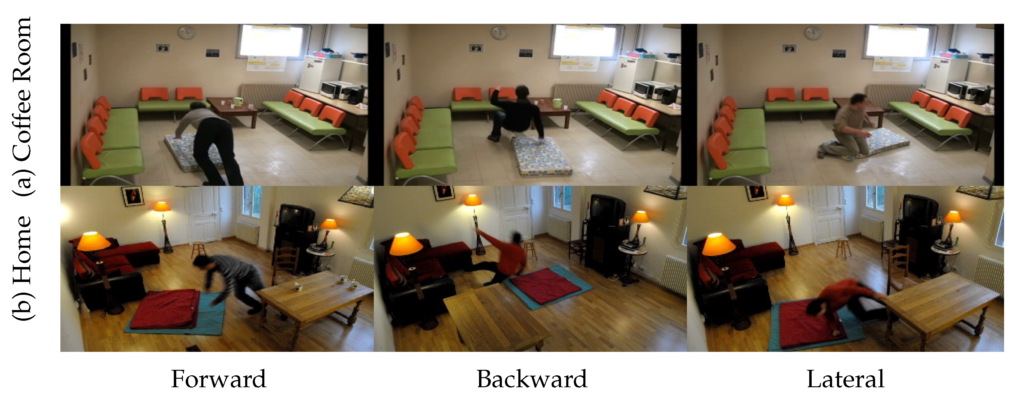
3.1. Dataset
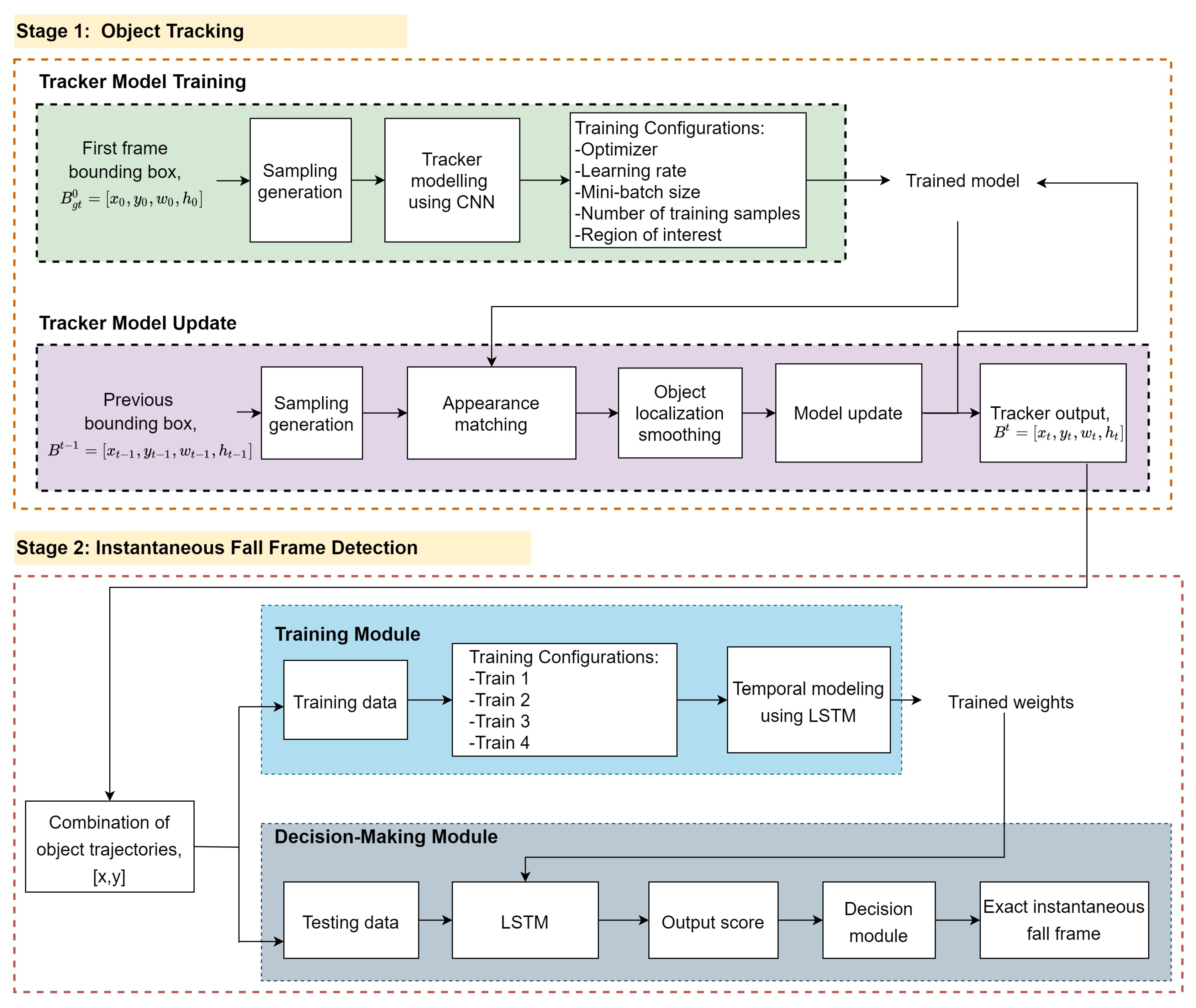
3.2. Stage 1: Object Tracking
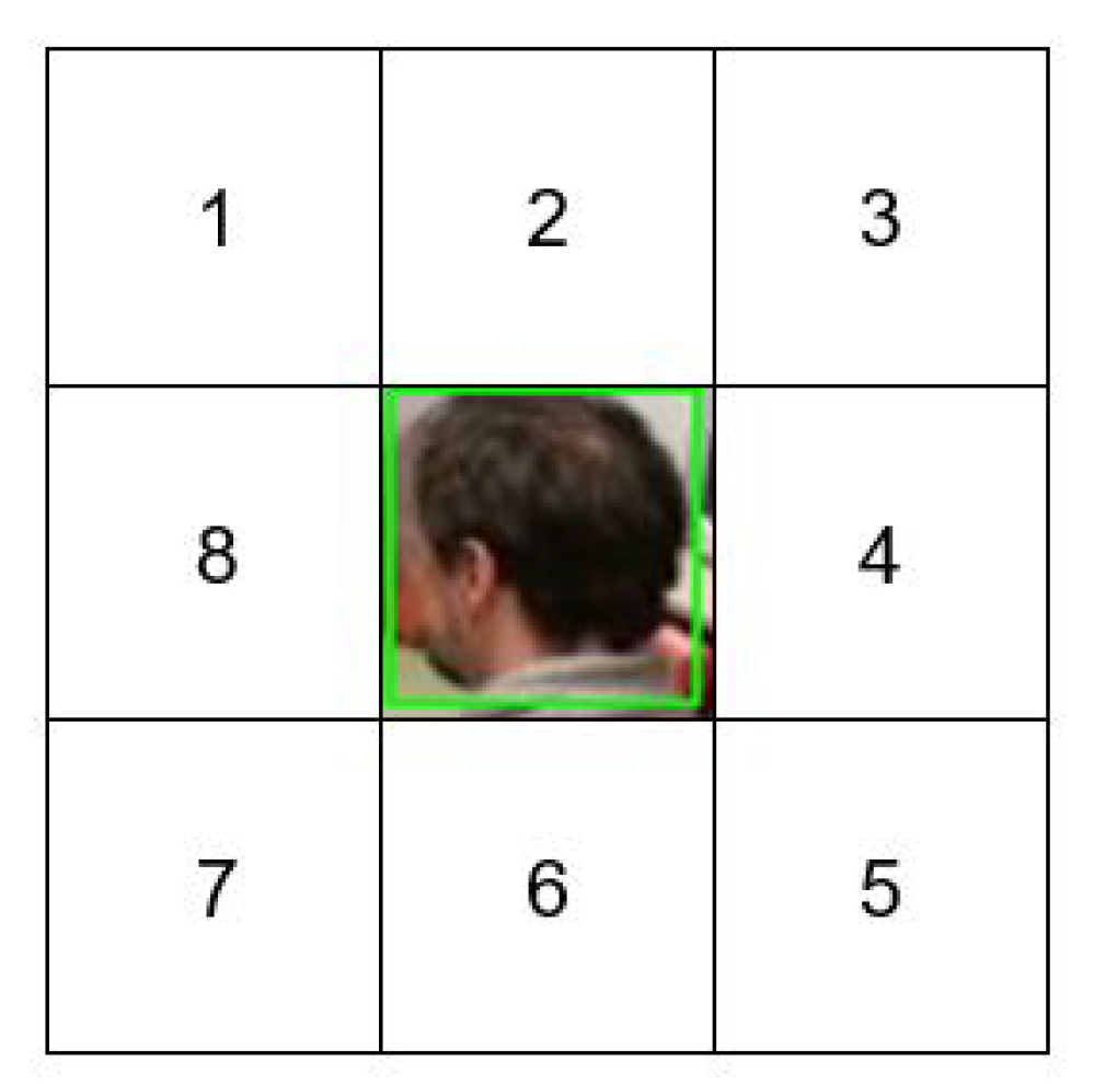
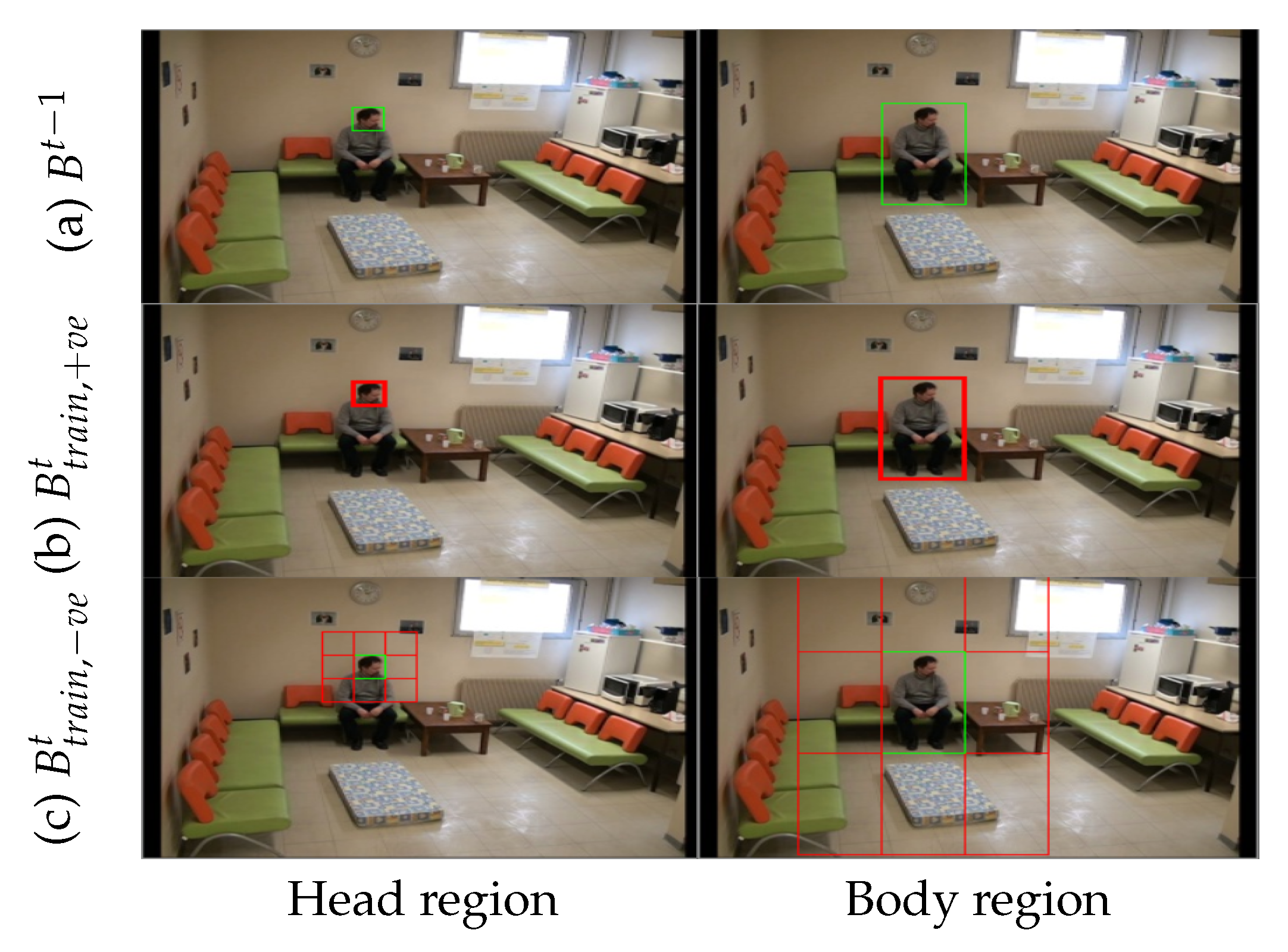
3.2.1. Sampling Generation
3.2.2. Tracker Model Training
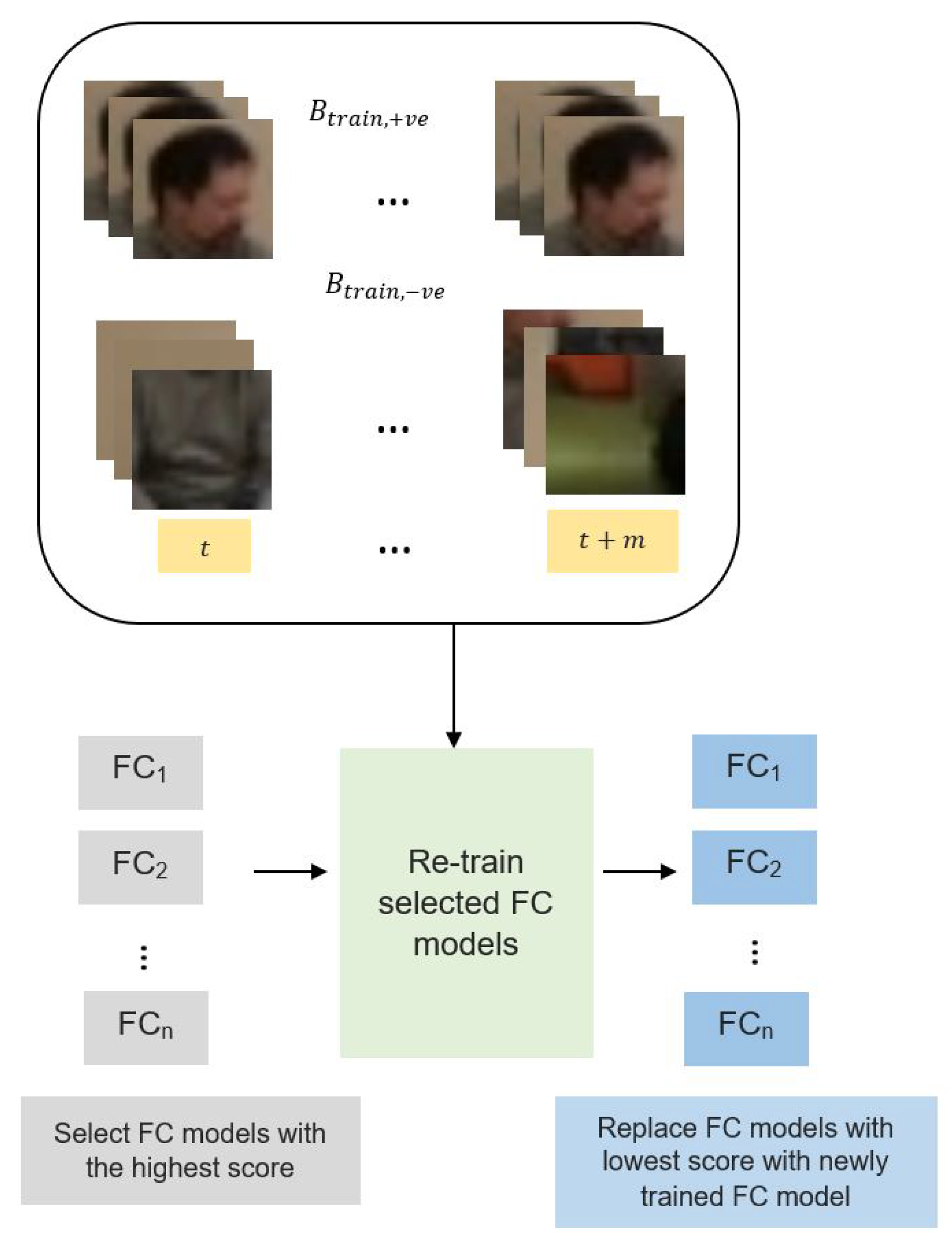
3.2.3. Tracker Model Update
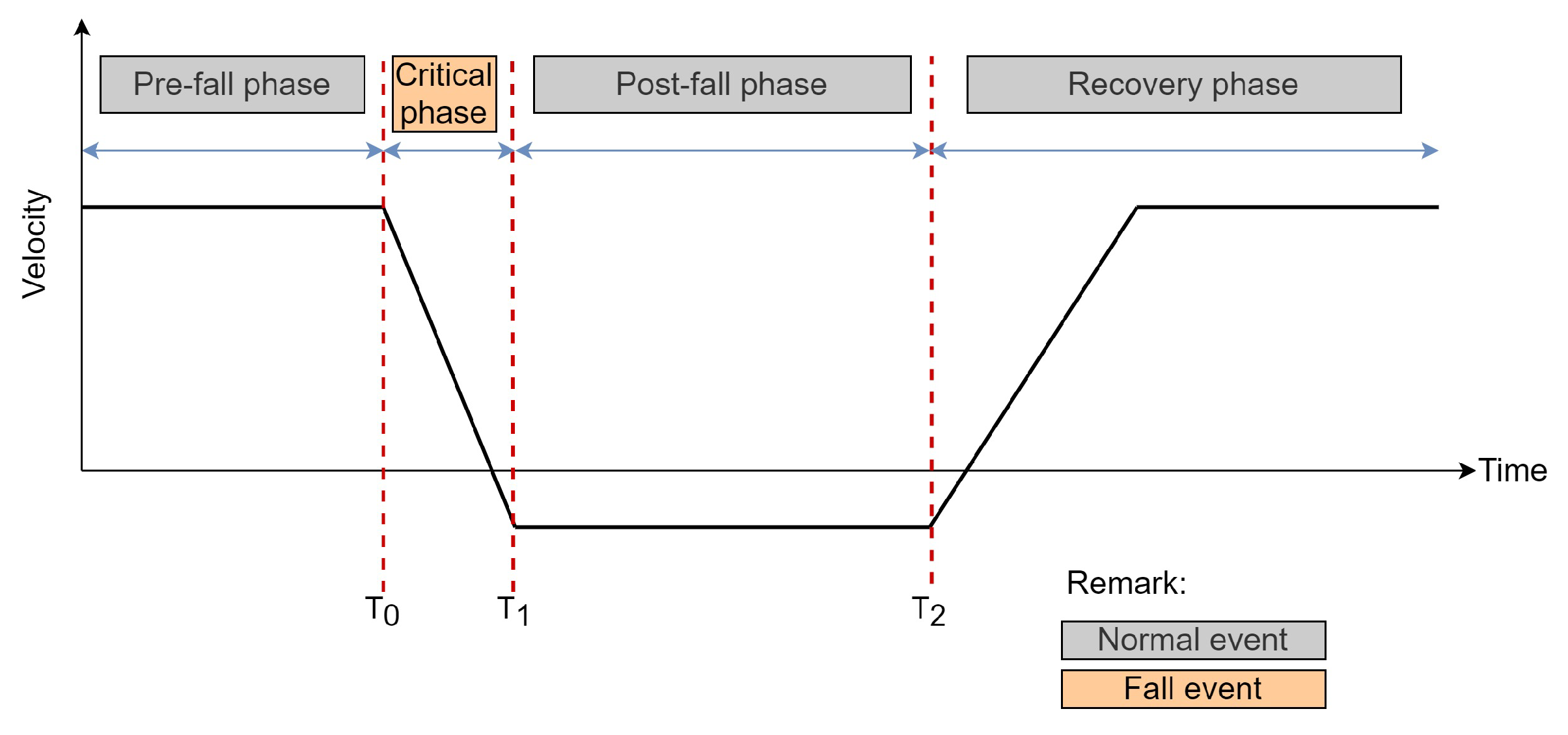
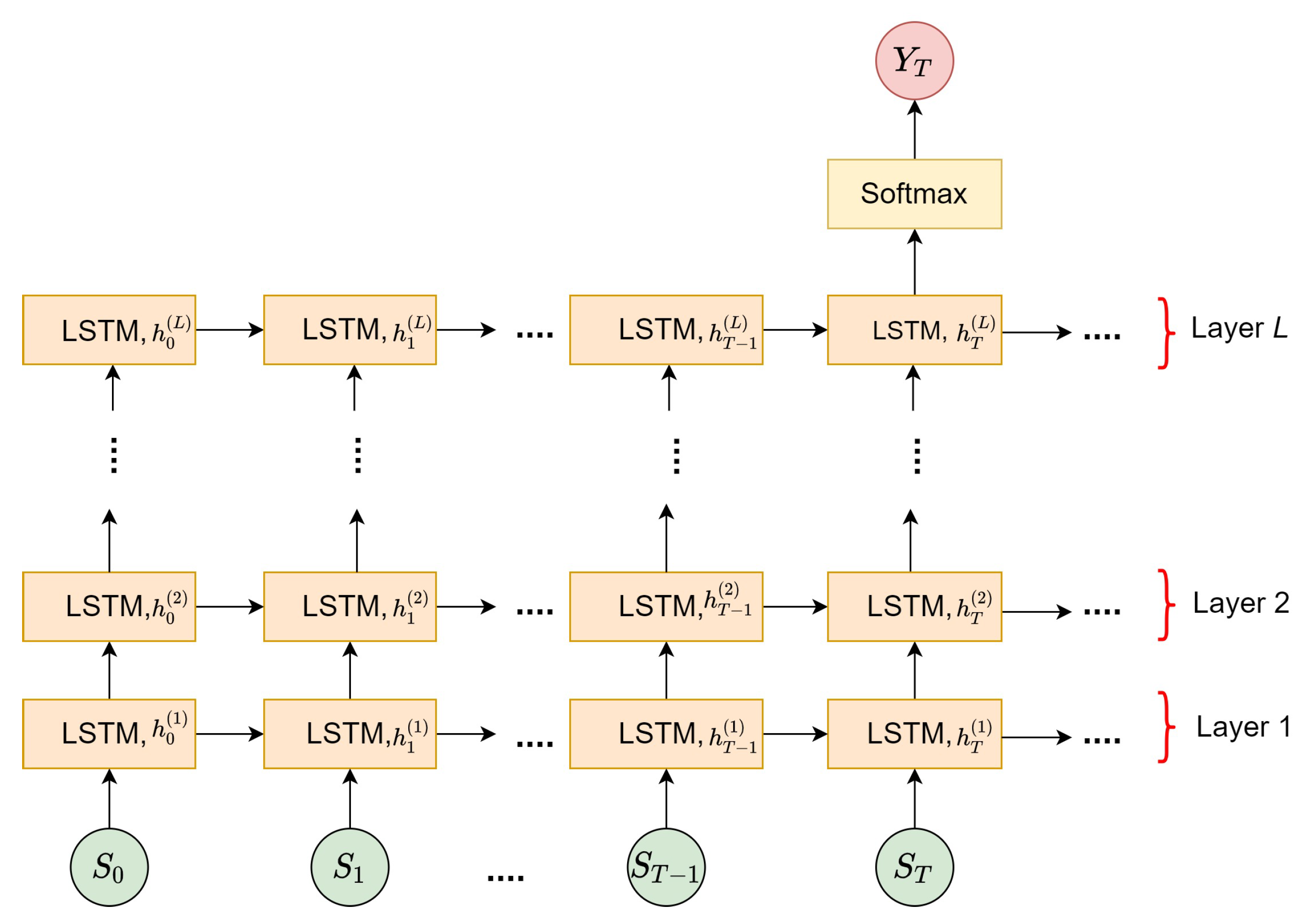
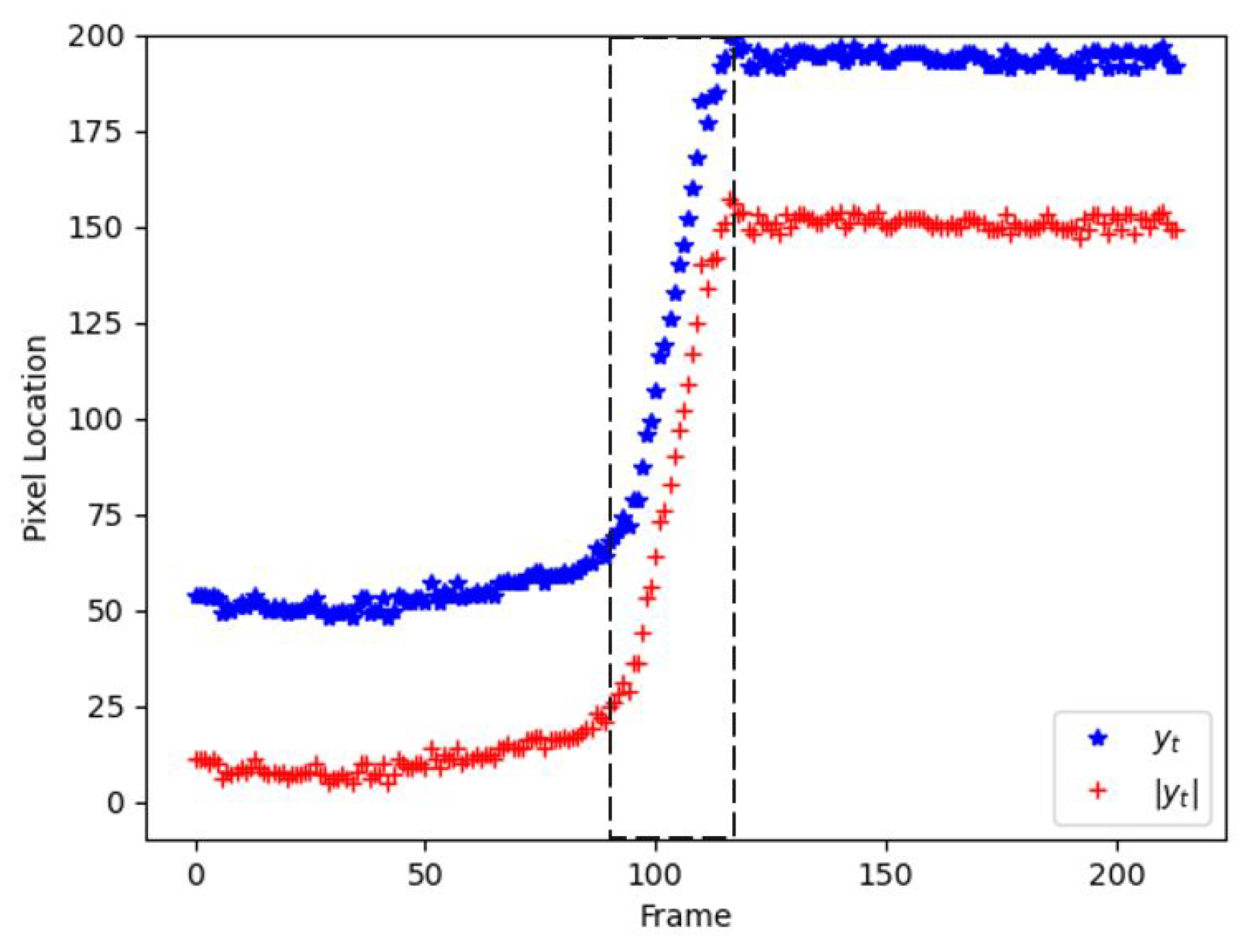
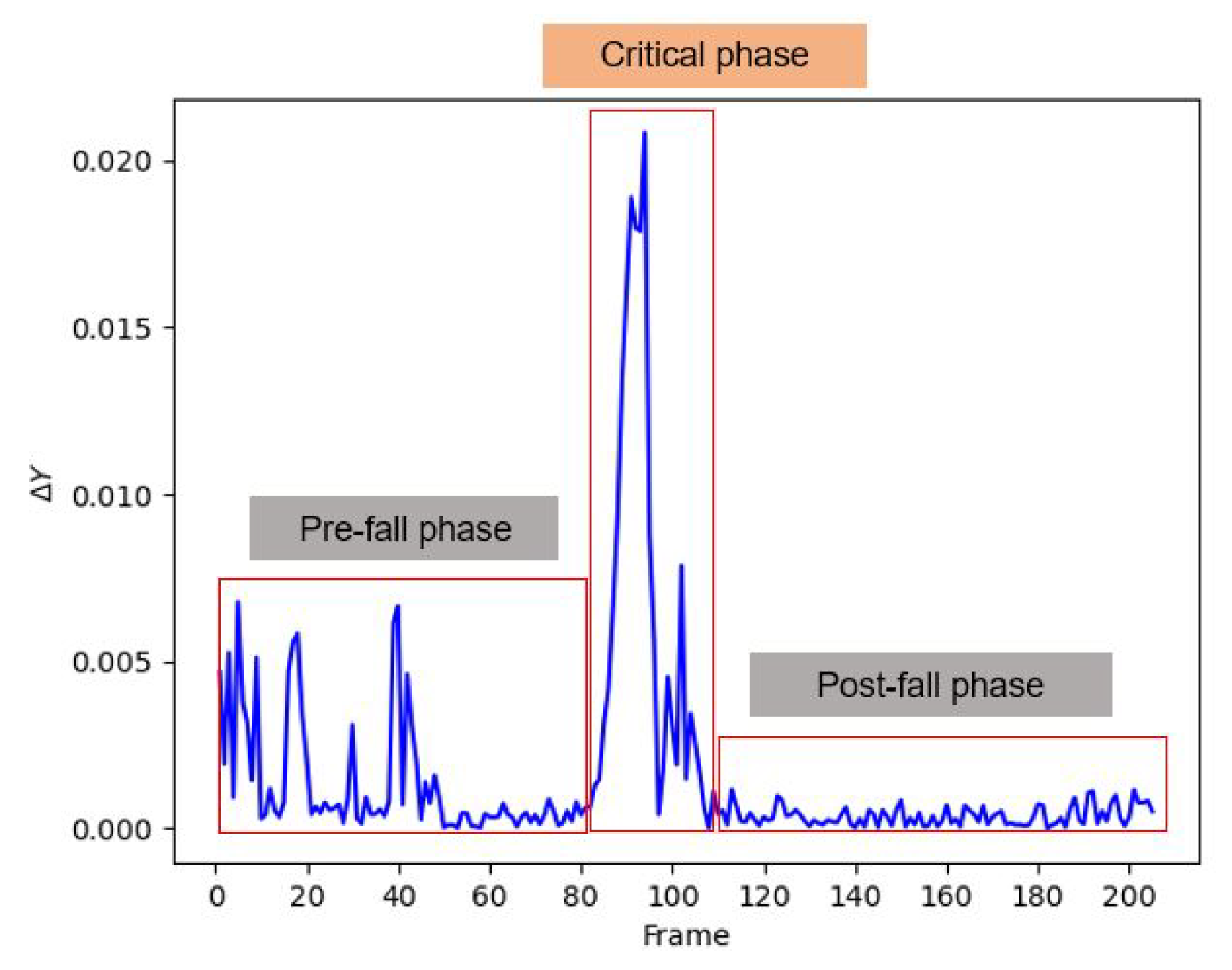
3.3. Stage 2: Instantaneous Fall Frame Detection
3.3.1. Training Module
3.3.2. Decision-Making Module
3.4. Performance Evaluation
4. Results
4.1. Results: Stage 1—Object Tracking Module
4.1.1. Optimizer
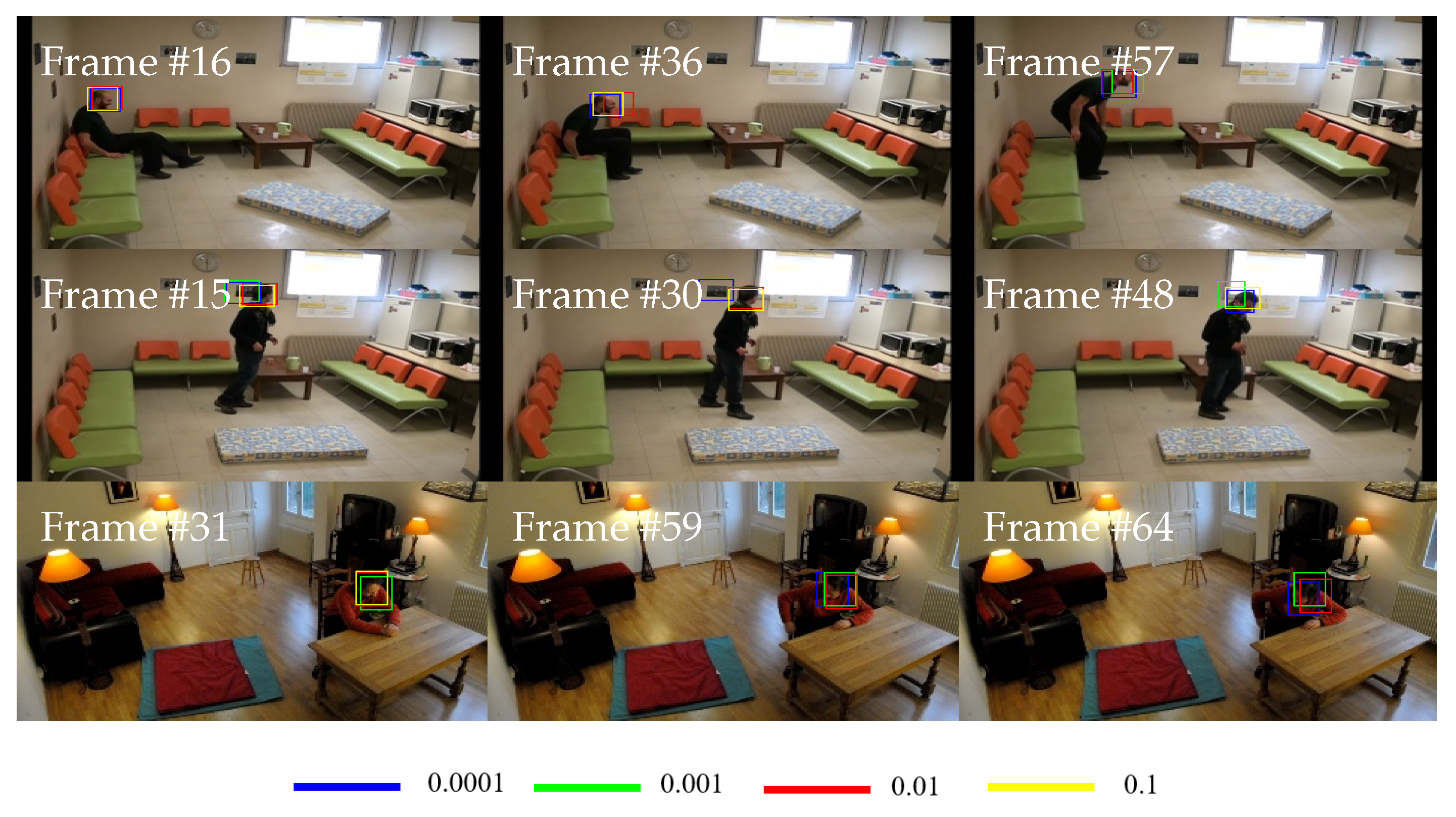
4.1.2. Learning Rate
4.1.3. Mini-Batch Size
4.1.4. No. of Training Samples
4.1.5. Region of Interest Selection
4.2. Results: Stage 2—Instantaneous Fall Frame Detection Module
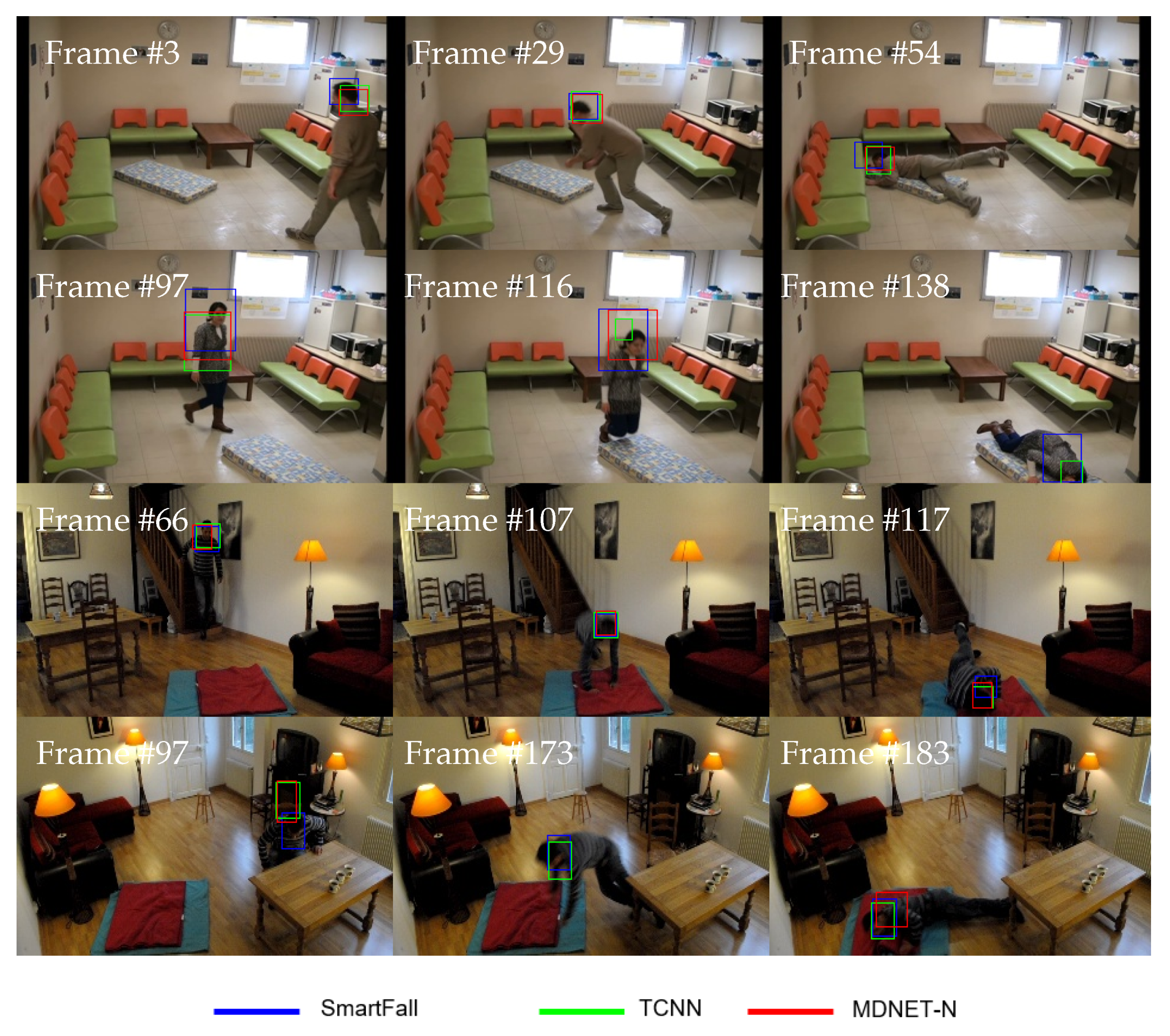
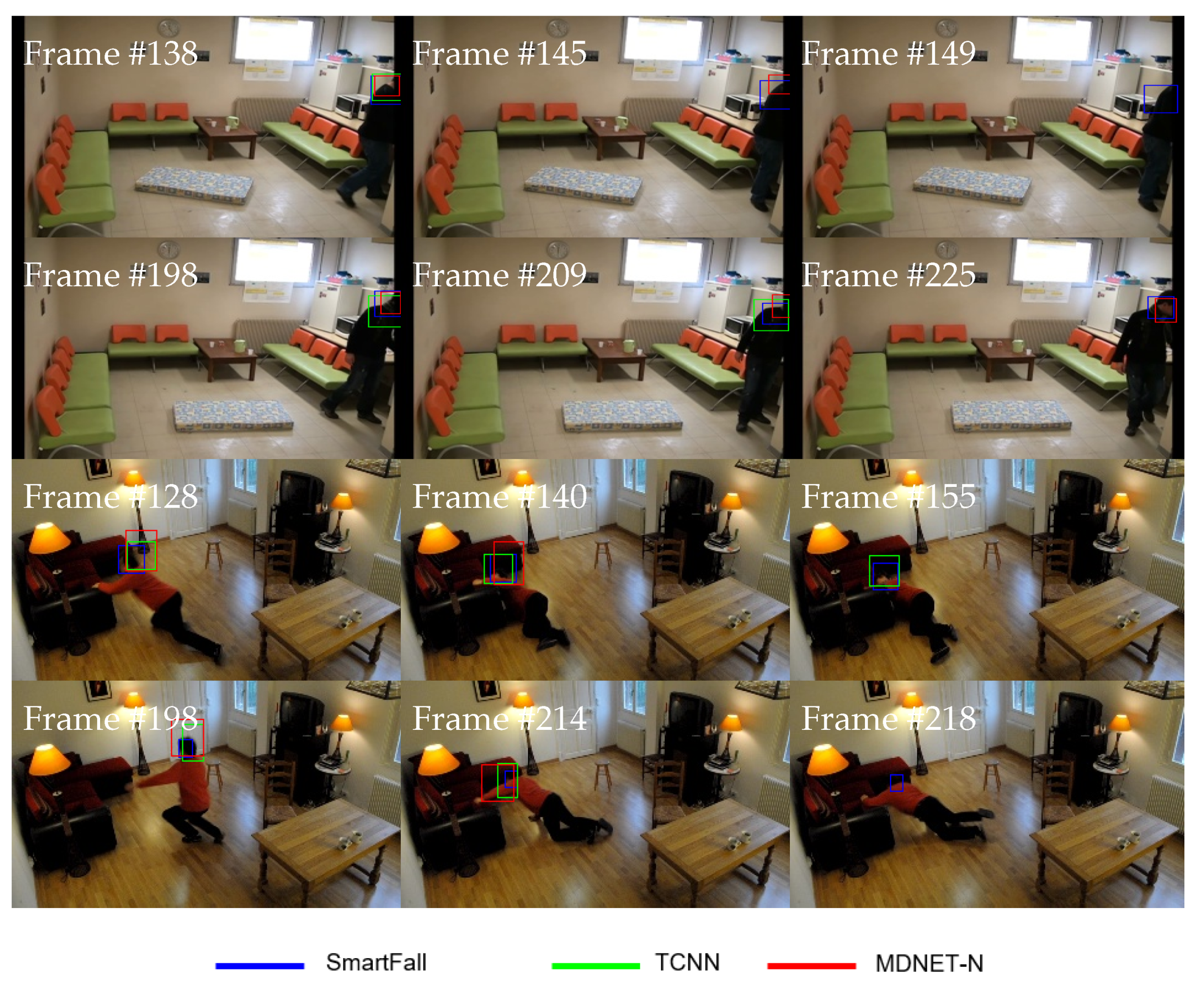
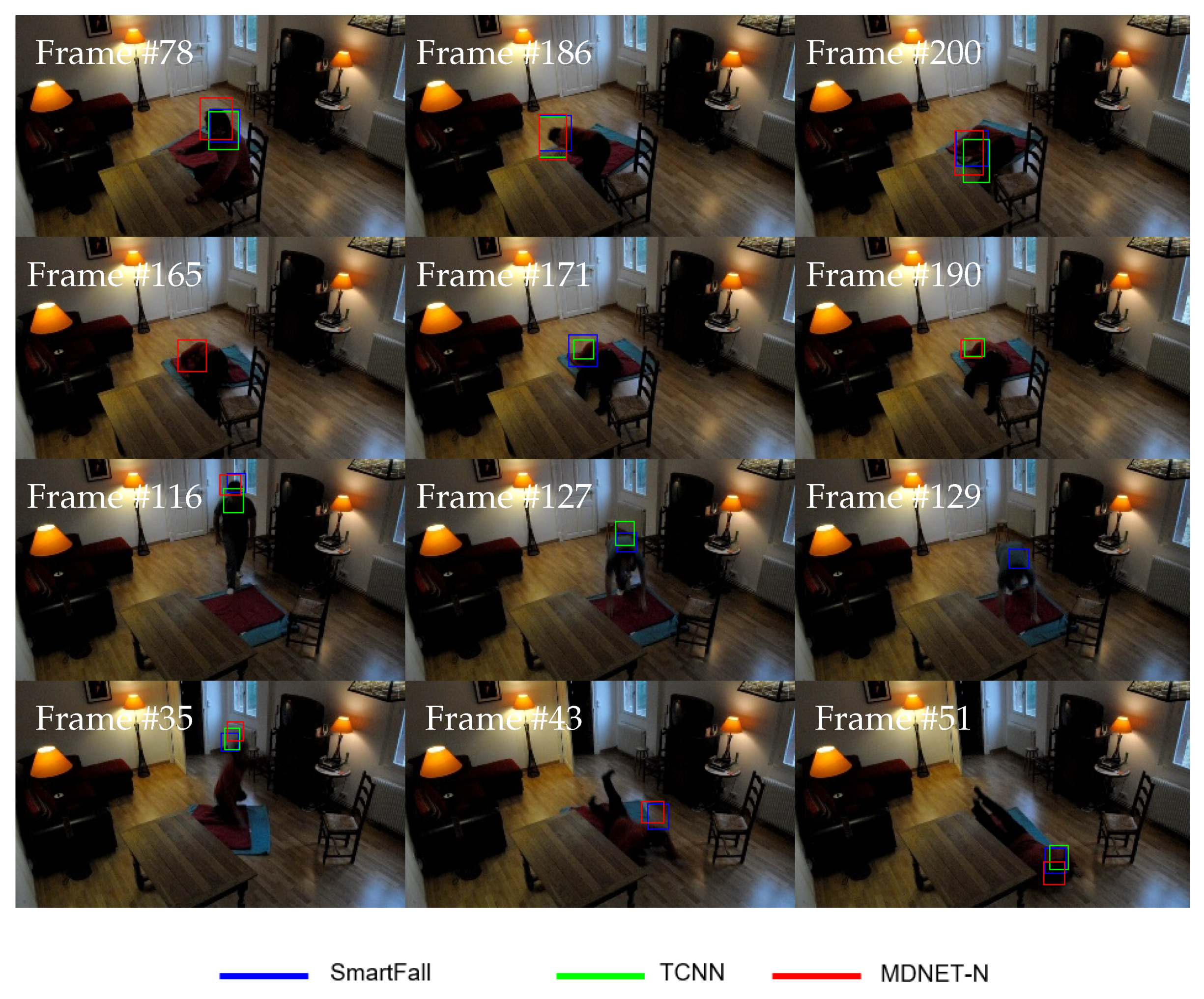
4.3. Benchmark Comparison
5. Discussion
6. Conclusions
Author Contributions
Funding
Institutional Review Board Statement
Informed Consent Statement
Data Availability Statement
Conflicts of Interest
Abbreviations
| CNN | Convolutional Neural Network |
| RNN | Recurrent Neural Network |
| LSTM | Long Short-Term Memory |
| GPU | Graphic Processing Unit |
| FDD | Fall Detection Dataset |
| CCTV | Closed Circuit Television |
| IP | Internet Protocol |
| MEMS | Microelectrical Mechanical System |
| WHO | World Health Organization |
| MDNET | Multi-Domain Convolutional Neural Network |
| TCNN | Tree-structured Convolutional Neural Network |
| VOT | Visual Object Tracking |
References
- Mabrouk, A.B.; Zagrouba, E. Abnormal behavior recognition for intelligent video surveillance systems: A review. Expert Syst. Appl. 2018, 91, 480–491. [Google Scholar] [CrossRef]
- Zhang, J.; Wu, C.; Wang, Y.; Wang, P. Detection of abnormal behavior in narrow scene with perspective distortion. Mach. Vis. Appl. 2019, 30, 987–998. [Google Scholar] [CrossRef]
- Khan, S.S.; Hoey, J. Review of fall detection techniques: A data availability perspective. Med. Eng. Phys. 2017, 39, 12–22. [Google Scholar] [CrossRef] [Green Version]
- Khan, S. Classification and Decision-Theoretic Framework for Detecting and Reporting Unseen Falls. Ph.D. Thesis, University of Waterloo, Waterloo, ON, Canada, 2016. [Google Scholar]
- WHO. The Health of Older People in Selected Countries of the Western Pacific Region; WHO Regional Office for the Western Pacific: Manila, Philippines, 2014. [Google Scholar]
- Makhlouf, A.; Boudouane, I.; Saadia, N.; Cherif, A.R. Ambient assistance service for fall and heart problem detection. J. Ambient. Intell. Humaniz. Comput. 2019, 10, 1527–1546. [Google Scholar] [CrossRef]
- Fortino, G.; Gravina, R. Fall-MobileGuard: A smart real-time fall detection system. In Proceedings of the 10th EAI International Conference on Body Area Networks, Sydney, Australia, 28–30 September 2015; pp. 44–50. [Google Scholar]
- WHO. WHO Global Report on Falls Prevention in Older Age; World Health Organization: Geneva, Switzerland, 2018. [Google Scholar]
- Non-Fatal Injuries at Work in Great Britain. Available online: https://www.hse.gov.uk/statistics/causinj/index.htm (accessed on 6 September 2021).
- Kinds of Accident Statistics in Great Britain. 2020. Available online: https://www.hse.gov.uk/statistics/causinj/kinds-of-accident.pdf (accessed on 6 September 2021).
- Ren, L.; Peng, Y. Research of Fall Detection and Fall Prevention Technologies: A Systematic Review. IEEE Access 2019, 7, 77702–77722. [Google Scholar] [CrossRef]
- Desai, K.; Mane, P.; Dsilva, M.; Zare, A.; Shingala, P.; Ambawade, D. A novel machine learning based wearable belt for fall detection. In Proceedings of the IEEE International Conference on Computing, Power and Communication Technologies (GUCON), Greater Noida, India, 2–4 October 2020; pp. 502–505. [Google Scholar]
- Britto Filho, J.C.; Lubaszewski, M. A Highly Reliable Wearable Device for Fall Detection. In Proceedings of the IEEE Latin-American Test Symposium (LATS), Maceio, Brazil, 30 March–2 April 2020; pp. 1–7. [Google Scholar]
- Oden, L.; Witt, T. Fall-detection on a wearable micro controller using machine learning algorithms. In Proceedings of the IEEE International Conference on Smart Computing (SMARTCOMP), Bologna, Italy, 14–17 September 2020; pp. 296–301. [Google Scholar]
- Lin, C.-L.; Chiu, W.-C.; Chen, F.-H.; Ho, Y.-H.; Chu, T.-C.; Hsieh, P.-H. Fall Monitoring for the Elderly Using Wearable Inertial Measurement Sensors on Eyeglasses. IEEE Sens. Lett. 2020, 4, 1–4. [Google Scholar] [CrossRef]
- González-Cañete, F.J.; Casilari, E. A feasibility study of the use of smartwatches in wearable fall detection systems. Sensors 2021, 21, 2254. [Google Scholar] [CrossRef] [PubMed]
- Ramanujam, E.; Padmavathi, S. Real time fall detection using infrared cameras and reflective tapes under day/night luminance. J. Ambient. Intell. Smart Environ. 2021, 13, 285–300. [Google Scholar] [CrossRef]
- Ogawa, Y.; Naito, K. Fall detection scheme based on temperature distribution with IR array sensor. In Proceedings of the IEEE International Conference on Consumer Electronics (ICCE), Las Vegas, NV, USA, 4–6 January 2020; pp. 1–5. [Google Scholar]
- Youngkong, P.; Panpanyatep, W. A Novel Double Pressure Sensors-Based Monitoring and Alarming System for Fall Detection. In Proceedings of the International Symposium on Instrumentation, Control, Artificial Intelligence, and Robotics (ICA-SYMP), Bangkok, Thailand, 20–22 January 2021; pp. 1–5. [Google Scholar]
- Li, S.; Xiong, H.; Diao, X. Pre-impact fall detection using 3D convolutional neural network. In Proceedings of the International Conference on Rehabilitation Robotics (ICORR), Toronto, ON, Canada, 24–28 June 2019; pp. 1173–1178. [Google Scholar]
- Lin, C.B.; Dong, Z.; Kuan, W.K.; Huang, Y.F. A Framework for Fall Detection Based on OpenPose Skeleton and LSTM/GRU Models. Appl. Sci. 2021, 11, 329. [Google Scholar] [CrossRef]
- Mobsite, S.; Alaoui, N.; Boulmalf, M. A framework for elders fall detection using deep learning. In Proceedings of the IEEE Congress on Information Science and Technology (CiSt), Agadir–Essaouira, Morocco, 5–12 June 2021; pp. 69–74. [Google Scholar]
- Taufeeque, M.; Koita, S.; Spicher, N.; Deserno, T.M. Multi-camera, multi-person, and real-time fall detection using long short term memory. In Proceedings of the Medical Imaging 2021: Imaging Informatics for Healthcare, Research, and Applications, Online, 15–20 February 2021; pp. 1–8. [Google Scholar]
- Solbach, M.D.; Tsotsos, J.K. Vision-based fallen person detection for the elderly. In Proceedings of the IEEE International Conference on Computer Vision Workshops, Venice, Italy, 22–29 October 2017; pp. 1433–1442. [Google Scholar]
- Dai, B.; Yang, D.; Ai, L.; Zhang, P. A Novel Video-Surveillance-Based Algorithm of Fall Detection. In Proceedings of the International Congress on Image and Signal Processing, BioMedical Engineering and Informatics (CISP-BMEI), Beijing, China, 13–15 October 2018; pp. 1–6. [Google Scholar]
- Debnath, A.; Kobra, K.T.; Rawshan, P.P.; Paramita, M.; Islam, M.N. An explication of acceptability of wearable devices in context of bangladesh: A user study. In Proceedings of the International Conference on Future Internet of Things and Cloud (FiCloud), Barcelona, Spain, 6–8 August 2018; pp. 136–140. [Google Scholar]
- Ismail, M.M.B.; Bchir, O. Automatic fall detection using membership based histogram descriptors. J. Comput. Sci. Technol. 2017, 32, 356–367. [Google Scholar] [CrossRef]
- Nizam, Y.; Mohd, M.N.H.; Jamil, M.M.A. A study on human fall detection systems: Daily activity classification and sensing techniques. Int. J. Integr. Eng. 2016, 8, 35–43. [Google Scholar]
- Khan, A.A.; Alsadoon, A.; Al-Khalisy, S.H.; Prasad, P.; Jerew, O.D.; Manoranjan, P. A Novel Hybrid Fall Detection Technique Using Body Part Tracking and Acceleration. In Proceedings of the International Conference on Innovative Technologies in Intelligent Systems and Industrial Applications (CITISIA), Sydney, Australia, 25–27 November 2020; pp. 1–8. [Google Scholar]
- Mohamed, N.A.; Zulkifley, M.A.; Kamari, N.A.M. Convolutional Neural Networks Tracker with Deterministic Sampling for Sudden Fall Detection. In Proceedings of the IEEE International Conference on System Engineering and Technology, Shah Alam, Malaysia, 7 October 2019; pp. 1–5. [Google Scholar]
- Krittanawong, C.; Zhang, H.; Wang, Z.; Aydar, M.; Kitai, T. Artificial intelligence in precision cardiovascular medicine. J. Am. Coll. Cardiol. 2017, 69, 2657–2664. [Google Scholar] [CrossRef]
- LeCun, Y.; Boser, B.E.; Denker, J.S.; Henderson, D.; Howard, R.E.; Hubbard, W.E.; Jackel, L.D. Handwritten digit recognition with a back-propagation network. In Advances in Neural Information Processing Systems; Morgan Kaufmann: Burlington, MA, USA, 1990; pp. 396–404. [Google Scholar]
- Voulodimos, A.; Doulamis, N.; Doulamis, A.; Protopapadakis, E. Deep learning for computer vision: A brief review. Comput. Intell. Neurosci. 2018, 2018, 7068349. [Google Scholar] [CrossRef] [PubMed]
- Mohamed, N.A.; Zulkifley, M.A.; Abdani, S.R. Spatial Pyramid Pooling with Atrous Convolutional for MobileNet. In Proceedings of the IEEE Student Conference on Research and Development (SCOReD), Batu Pahat, Malaysia, 27–29 October 2020; pp. 333–336. [Google Scholar]
- Zhai, M.; Chen, L.; Mori, G.; Javan Roshtkhari, M. Deep learning of appearance models for online object tracking. In Proceedings of the European Conference on Computer Vision (ECCV), Munich, Germany, 8–14 September 2018; pp. 1–6. [Google Scholar]
- Nam, H.; Baek, M.; Han, B. Modeling and propagating cnns in a tree structure for visual tracking. arXiv 2016, arXiv:1608.07242. [Google Scholar]
- Nam, H.; Han, B. Learning multi-domain convolutional neural networks for visual tracking. In Proceedings of the IEEE Conference on Computer Vision and Pattern Recognition, Las Vegas, NV, USA, 18–20 June 2016; pp. 4293–4302. [Google Scholar]
- Zulkifley, M.A.; Rawlinson, D.; Moran, B. Robust observation detection for single object tracking: Deterministic and probabilistic patch-based approaches. Sensors 2012, 12, 15638–15670. [Google Scholar] [CrossRef] [PubMed]
- Tiwari, G.; Sharma, A.; Sahotra, A.; Kapoor, R. English-Hindi neural machine translation-LSTM seq2seq and ConvS2S. In Proceedings of the International Conference on Communication and Signal Processing (ICCSP), Chennai, India, 28–30 July 2020; pp. 871–875. [Google Scholar]
- Su, C.; Huang, H.; Shi, S.; Jian, P.; Shi, X. Neural machine translation with Gumbel tree-LSTM based encoder. J. Vis. Commun. Image Represent. 2020, 71, 102811. [Google Scholar] [CrossRef]
- Vathsala, M.K.; Holi, G. RNN based machine translation and transliteration for Twitter data. Int. J. Speech Technol. 2020, 23, 499–504. [Google Scholar] [CrossRef]
- Jin, N.; Wu, J.; Ma, X.; Yan, K.; Mo, Y. Multi-task learning model based on multi-scale CNN and LSTM for sentiment classification. IEEE Access 2020, 8, 77060–77072. [Google Scholar] [CrossRef]
- Huang, X.; Zhang, W.; Huang, Y.; Tang, X.; Zhang, M.; Surbiryala, J.; Iosifidis, V.; Liu, Z.; Zhang, J. LSTM Based Sentiment Analysis for Cryptocurrency Prediction. arXiv 2021, arXiv:2103.14804. [Google Scholar]
- Di Gennaro, G.; Buonanno, A.; Di Girolamo, A.; Palmieri, F.A. Intent classification in question-answering using LSTM architectures. In Artificial Intelligence and Neural Systems; Springer: Singapore, 2021; pp. 115–124. [Google Scholar]
- Mehtab, S.; Sen, J.; Dutta, A. Stock price prediction using machine learning and LSTM-based deep learning models. In Proceedings of the Symposium on Machine Learning and Metaheuristics Algorithms, and Applications, Chennai, India, 14–17 October 2020; pp. 88–106. [Google Scholar]
- Sunny, M.A.I.; Maswood, M.M.S.; Alharbi, A.G. Deep Learning-Based Stock Price Prediction Using LSTM and Bi-Directional LSTM Model. In Proceedings of the Novel Intelligent and Leading Emerging Sciences Conference (NILES), Giza, Egypt, 24–26 October 2020; pp. 87–92. [Google Scholar]
- Ayan, E.; Eken, S. Detection of price bubbles in Istanbul housing market using LSTM autoencoders: A district-based approach. Soft Comput. 2021, 25, 7957–7973. [Google Scholar] [CrossRef]
- Karevan, Z.; Suykens, J.A. Transductive LSTM for time-series prediction: An application to weather forecasting. Neural Netw. 2020, 125, 1–9. [Google Scholar] [CrossRef]
- Sultana, A.; Deb, K.; Dhar, P.K.; Koshiba, T. Classification of indoor human fall events using deep learning. Entropy 2021, 23, 328. [Google Scholar] [CrossRef] [PubMed]
- Abdo, H.; Amin, K.M.; Hamad, A.M. Fall Detection Based on RetinaNet and MobileNet Convolutional Neural Networks. In Proceedings of the International Conference on Computer Engineering and Systems (ICCES), Cairo, Egypt, 15–16 December 2020; pp. 1–7. [Google Scholar]
- Yao, C.; Hu, J.; Min, W.; Deng, Z.; Zou, S.; Min, W. A novel real-time fall detection method based on head segmentation and convolutional neural network. J. Real-Time Image Process. 2020, 17, 1939–1949. [Google Scholar] [CrossRef]
- Iazzi, A.; Rziza, M.; Thami, R.O.H. Fall Detection System-Based Posture-Recognition for Indoor Environments. J. Imaging 2021, 7, 42. [Google Scholar] [CrossRef] [PubMed]
- Chen, Y.; Li, W.; Wang, L.; Hu, J.; Ye, M. Vision-based fall event detection in complex background using attention guided bi-directional LSTM. IEEE Access 2020, 8, 161337–161348. [Google Scholar] [CrossRef]
- Kakiuchi, Y.; Nagao, R.; Ochiai, E.; Kakimoto, Y.; Osawa, M. The impact of discontinuation of the medical examiner system: Cases of drowning in the bathtub at home. J. Forensic Sci. 2020, 65, 974–978. [Google Scholar] [CrossRef] [PubMed]
- McCall, J.D.; Sternard, B.T. Drowning; StatPearls Publishing: Treasure Island, FL, USA, 2020. [Google Scholar]
- Muad, A.M.; Zaki, S.K.M.; Jasim, S.A. Optimizing hopfield neural network for super-resolution mapping. J. Kejuruter. 2020, 32, 91–97. [Google Scholar]
- Yu, M.; Gong, L.; Kollias, S. Computer vision based fall detection by a convolutional neural network. In Proceedings of the International Conference on Multimodal Interaction, Glasgow, UK, 13–17 November 2017; pp. 416–420. [Google Scholar]
- Adhikari, K.; Bouchachia, H.; Nait-Charif, H. Activity recognition for indoor fall detection using convolutional neural network. In Proceedings of the International Conference on Machine Vision Applications (MVA), Nagoya, Japan, 8–12 May 2017; pp. 81–84. [Google Scholar]
- Li, X.; Pang, T.; Liu, W.; Wang, T. Fall detection for elderly person care using convolutional neural networks. In Proceedings of the International Congress on Image and Signal Processing, BioMedical Engineering and Informatics (CISP-BMEI), Shanghai, China, 14–16 October 2017; pp. 1–6. [Google Scholar]
- Abdani, S.R.; Zulkifley, M.A. Compact convolutional neural networks for pterygium classification using transfer learning. In Proceedings of the IEEE International Conference on Signal and Image Processing Applications (ICSIPA), Kuala Lumpur, Malaysia, 17–19 September 2019; pp. 140–143. [Google Scholar]
- Min, W.; Cui, H.; Rao, H.; Li, Z.; Yao, L. Detection of human falls on furniture using scene analysis based on deep learning and activity characteristics. IEEE Access 2018, 6, 9324–9335. [Google Scholar] [CrossRef]
- Feng, Q.; Gao, C.; Wang, L.; Zhang, M.; Du, L.; Qin, S. Fall detection based on motion history image and histogram of oriented gradient feature. In Proceedings of the International Symposium on Intelligent Signal Processing and Communication Systems (ISPACS), Xiamen, China, 6–9 November 2017; pp. 341–346. [Google Scholar]
- Núñez-Marcos, A.; Azkune, G.; Arganda-Carreras, I. Vision-based fall detection with convolutional neural networks. Wirel. Commun. Mob. Comput. 2017, 2017, 1–16. [Google Scholar] [CrossRef] [Green Version]
- Han, Q.; Zhao, H.; Min, W.; Cui, H.; Zhou, X.; Zuo, K.; Liu, R. A two-stream approach to fall detection with mobilevgg. IEEE Access 2020, 8, 17556–17566. [Google Scholar] [CrossRef]
- Shojaei-Hashemi, A.; Nasiopoulos, P.; Little, J.J.; Pourazad, M.T. Video-based human fall detection in smart homes using deep learning. In Proceedings of the IEEE International Symposium on Circuits and Systems (ISCAS), Florence, Italy, 27–30 May 2018; pp. 1–5. [Google Scholar]
- Charfi, I.; Miteran, J.; Dubois, J.; Atri, M.; Tourki, R. Optimized spatio-temporal descriptors for real-time fall detection: Comparison of support vector machine and Adaboost-based classification. J. Electron. Imaging 2013, 22, 041106. [Google Scholar] [CrossRef]
- Chatfield, K.; Simonyan, K.; Vedaldi, A.; Zisserman, A. Return of the devil in the details: Delving deep into convolutional nets. arXiv 2014, arXiv:1405.3531. [Google Scholar]
- Zulkifley, M.A.; Trigoni, N. Multiple-model fully convolutional neural networks for single object tracking on thermal infrared video. IEEE Access 2018, 6, 42790–42799. [Google Scholar] [CrossRef]
- Kingma, D.P.; Ba, J. Adam: A method for stochastic optimization. arXiv 2014, arXiv:1412.6980. [Google Scholar]
- Duchi, J.; Hazan, E.; Singer, Y. Adaptive subgradient methods for online learning and stochastic optimization. J. Mach. Learn. Res. 2011, 12, 2121–2159. [Google Scholar]
- Robbins, H.; Monro, S. A stochastic approximation method. Ann. Math. Stat. 1951, 22, 400–407. [Google Scholar] [CrossRef]
- Zeiler, M.D. Adadelta: An adaptive learning rate method. arXiv 2012, arXiv:1212.5701. [Google Scholar]
- Hinton, G.; Srivastava, N. Swersky, K. Neural networks for machine learning lecture 6a overview of mini-batch gradient descent. Cited On 2012, 14, 2. [Google Scholar]
- Abbate, S.; Avvenuti, M.; Corsini, P.; Light, J.; Vecchio, A. Monitoring of human movements for fall detection and activities recognition in elderly care using wireless sensor network: A survey. In Wireless Sensor Networks: Application-Centric Design; IntechOpen: Rijeka, Croatia, 2010; pp. 147–166. [Google Scholar]
- Manaswi, N.K. RNN and LSTM. In Deep Learning with Applications Using Python; Springer: Berkeley, CA, USA, 2018; pp. 115–126. [Google Scholar]
- Kristan, M.; Leonardis, A.; Matas, J.; Felsberg, M.; Pflugfelder, R.; Cehovin Zajc, L.; Vojir, T.; Bhat, G.; Lukezic, A.; Eldesokey, A.; et al. The sixth visual object tracking vot2018 challenge results. In Proceedings of the European Conference on Computer Vision (ECCV), Munich, Germany, 8–14 September 2018; pp. 1–52. [Google Scholar]
- Krizhevsky, A.; Sutskever, I.; Hinton, G.E. Imagenet classification with deep convolutional neural networks. Adv. Neural Inf. Process. Syst. 2012, 2, 1097–1105. [Google Scholar] [CrossRef]
- Martínez-Villaseñor, L.; Ponce, H.; Perez-Daniel, K. Deep learning for multimodal fall detection. In Proceedings of the IEEE International Conference on Systems, Man and Cybernetics (SMC), Bari, Italy, 6–9 October 2019; pp. 3422–3429. [Google Scholar]
- Abdani, S.R.; Zulkifley, M.A. Optimal Selection of Pyramid Pooling Components for Convolutional Neural Network Classifier. In Proceedings of the International Conference on Decision Aid Sciences and Application (DASA), Sakheer, Bahrain, 8–9 November 2020; pp. 586–591. [Google Scholar]
- Adhikari, K.; Bouchachia, H.; Nait-Charif, H. Deep learning based fall detection using simplified human posture. Int. J. Comput. Syst. Eng. 2019, 13, 251–256. [Google Scholar]


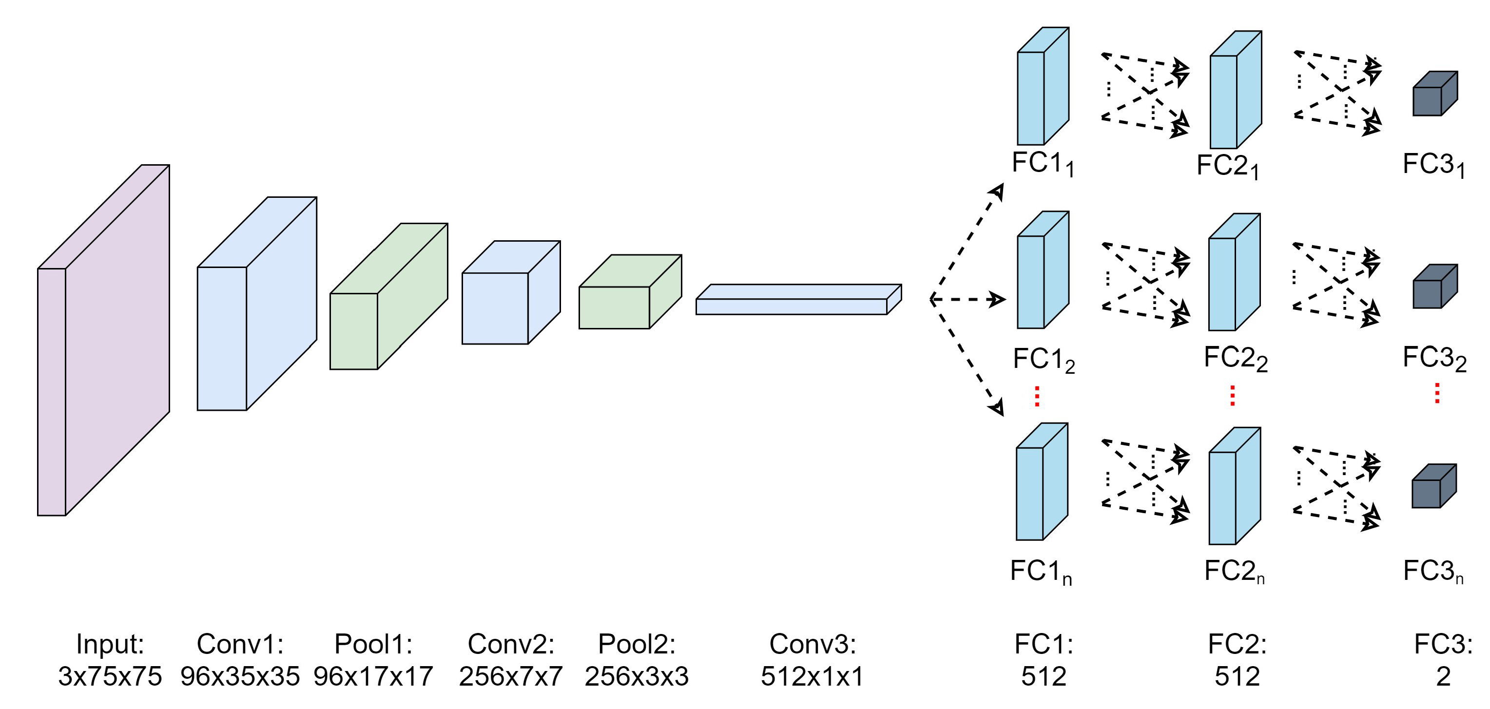
| Layer | Filter Size | Stride | Padding | Output | Activation Function |
|---|---|---|---|---|---|
| Conv1 | 2 | 0 | ReLU | ||
| Pool1 | 2 | 0 | - | ||
| Conv2 | 2 | 0 | ReLU | ||
| Pool2 | 2 | 0 | - | ||
| Conv3 | 1 | 0 | ReLU | ||
| FC1 | - | - | - | 512 | ReLU |
| FC2 | - | - | - | 512 | ReLU |
| FC3 | - | - | - | 2 | Softmax |
| Hyperparameter | Type/Value | Function |
|---|---|---|
| Optimizer | Adam AdaGrad SGD AdaDelta RMSProp | Method to update parameters to reduce losses during training process |
| Learning rate | 0.0001 0.001 0.01 0.1 | Step size to update weights with respect to the gradient loss |
| Mini-batch size | 64 128 256 | The number of training samples for each training iteration |
| Number of training samples | 400 600 800 | Total candidate samples of and |
| Parameter | Value |
|---|---|
| 50 | |
| 200 | |
| 0.1 | |
| 2 |
| Training Configuration | Description |
|---|---|
| Train-1 | |
| Train-2 | + dropout |
| Train-3 | |
| Train-4 | + dropout |
| Learning Rate = 0.001 Mini-Batch Size = 128 No. of Training Samples = 400 | ||||||||||
|---|---|---|---|---|---|---|---|---|---|---|
| Head | Body | |||||||||
| Type | EAO | Ac | Ro | Re | Ffail | EAO | Ac | Ro | Re | Ffail |
| Adam | 0.1668 | 0.4415 | 0.4493 | 0.8557 | 31 | 0.1653 | 0.4554 | 0.4493 | 0.8384 | 31 |
| AdaGrad | 0.1288 | 0.4377 | 0.9855 | 0.7091 | 68 | 0.1457 | 0.4306 | 0.6232 | 0.7799 | 43 |
| SGD | 0.1092 | 0.3964 | 1.0290 | 0.6784 | 71 | 0.1583 | 0.4314 | 0.5072 | 0.8132 | 35 |
| AdaDelta | 0.0404 | 0.3014 | 3.8382 | 0.2599 | 261 | 0.0637 | 0.2878 | 1.7059 | 0.5470 | 116 |
| RMSProp | 0.1543 | 0.4680 | 0.8695 | 0.5074 | 60 | 0.1708 | 0.4716 | 0.4928 | 0.8221 | 34 |
| Optimizer = Adam Mini-Batch Size = 128 No. of Training Samples = 400 | ||||||||||
|---|---|---|---|---|---|---|---|---|---|---|
| Head | Body | |||||||||
| Value | EAO | Ac | Ro | Re | Ffail | EAO | Ac | Ro | Re | Ffail |
| 0.0001 | 0.1669 | 0.4869 | 0.5652 | 0.8248 | 39 | 0.1898 | 0.4883 | 0.3623 | 0.8645 | 25 |
| 0.001 | 0.1651 | 0.4415 | 0.4493 | 0.8557 | 31 | 0.1653 | 0.4554 | 0.4492 | 0.8384 | 31 |
| 0.01 | 0.1693 | 0.4757 | 0.4783 | 0.8339 | 33 | 0.1785 | 0.4756 | 0.3913 | 0.8504 | 27 |
| 0.1 | 0.0788 | 0.4060 | 2.3478 | 0.4229 | 162 | 0.1089 | 0.4030 | 1.2319 | 0.6370 | 85 |
| Optimizer = Adam No. of Training Sample = 400 Learning Rate = 0.0001 | ||||||||||
|---|---|---|---|---|---|---|---|---|---|---|
| Head | Body | |||||||||
| Value | EAO | Ac | Ro | Re | Ffail | EAO | Ac | Ro | Re | Ffail |
| 64 | 0.1679 | 0.4719 | 0.5072 | 0.8304 | 35 | 0.1683 | 0.4563 | 0.4782 | 0.8268 | 33 |
| 128 | 0.1669 | 0.4415 | 0.4493 | 0.8557 | 31 | 0.1653 | 0.4554 | 0.4493 | 0.8384 | 31 |
| 256 | 0.1594 | 0.4633 | 0.4928 | 0.8327 | 34 | 0.1665 | 0.4596 | 0.4493 | 0.8349 | 31 |
| Optimizer = Adam Mini-Batch Size = 128 Learning Rate = 0.0001 | ||||||||||
|---|---|---|---|---|---|---|---|---|---|---|
| Head | Body | |||||||||
| Value | EAO | Ac | Ro | Re | Ffail | EAO | Ac | Ro | Re | Ffail |
| 400 | 0.1669 | 0.4415 | 0.4493 | 0.8557 | 31 | 0.1653 | 0.4554 | 0.4493 | 0.8384 | 31 |
| 600 | 0.1606 | 0.4462 | 0.5217 | 0.8349 | 36 | 0.1664 | 0.4618 | 0.4638 | 0.8277 | 32 |
| 800 | 0.1538 | 0.4407 | 0.6232 | 0.7930 | 43 | 0.1644 | 0.4581 | 0.4638 | 0.8329 | 32 |
| Head | Body | |
|---|---|---|
| EAO | 0.1718 | 0.1619 |
| Ac | 0.4871 | 0.4659 |
| Ro | 0.4706 | 0.6324 |
| Re | 0.8274 | 0.7958 |
| 32 | 42 |
| Configuration | RNN | Stacked LSTM | ||||||
|---|---|---|---|---|---|---|---|---|
| F1 | 36 | 32 | 29 | 33 | 32 | 35 | 30 | 44 |
| F2 | 36 | 35 | 33 | 28 | 28 | 31 | 41 | 43 |
| F3 | 43 | 36 | 26 | 29 | 30 | 32 | 36 | 37 |
| F4 | 40 | 33 | 26 | 22 | 27 | 32 | 37 | 39 |
| Method | Training Accuracy (%) | Training Loss | Training Duration |
|---|---|---|---|
| RNN | 59.17 | 3.1578 | 1 h 4 min |
| Stacked LSTM: | |||
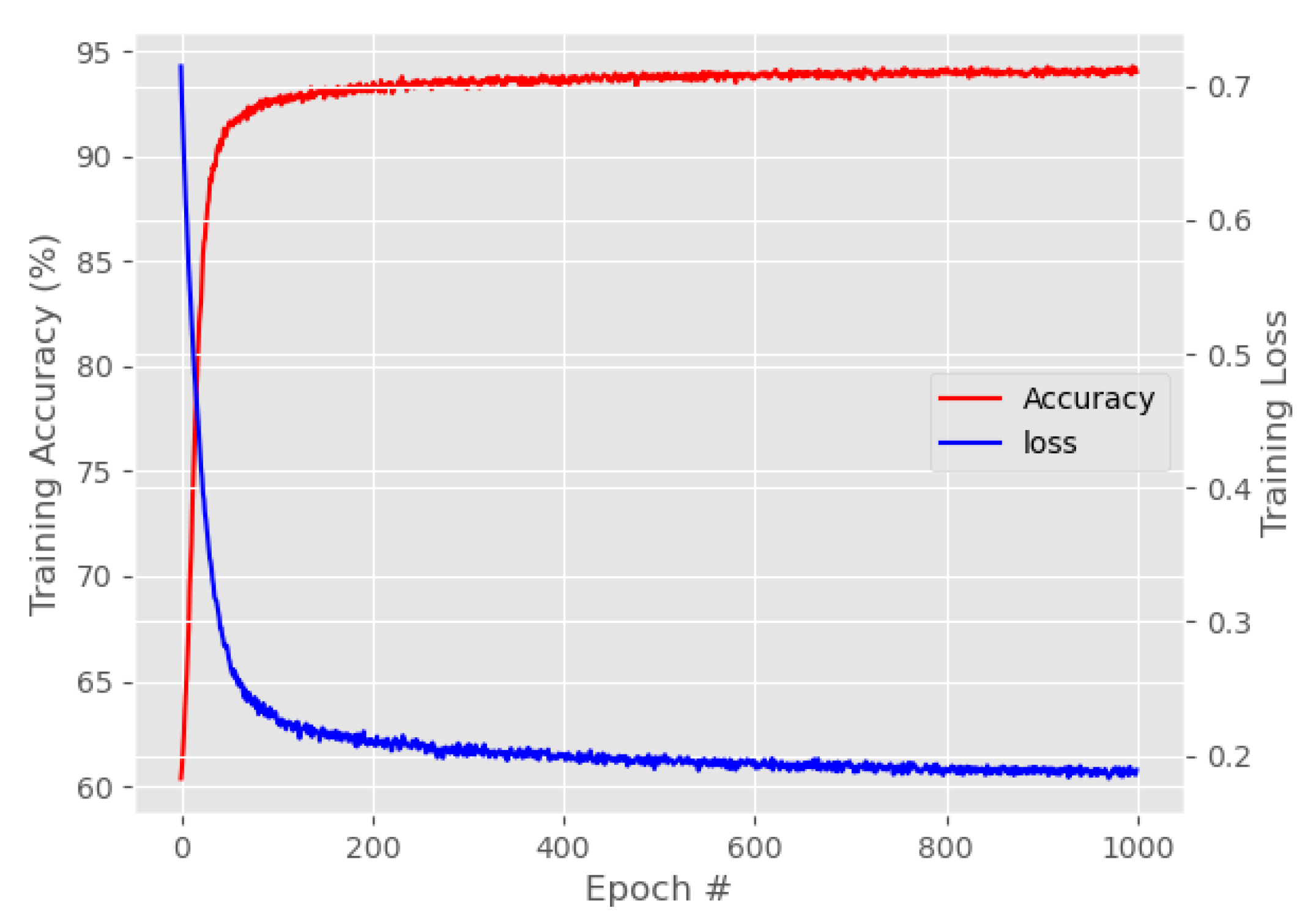
| 76.56 | 0.7146 | 2 h 44 min | |
| 91.32 | 0.2413 | 3 h 17 min | |
| 93.01 | 0.2112 | 4 h 10 min | |
| 92.05 | 0.2261 | 5 h 6 min | |
| 91.27 | 0.2445 | 5 h 36 min | |
| 90.95 | 0.2470 | 6 h 29 min | |
| 89.88 | 0.2666 | 7 h 23 min |
| Tracker | EAO | Ac | Ro | Re | Ffail |
|---|---|---|---|---|---|
| SmartConvFall | 0.1619 | 0.4659 | 0.6323 | 0.7958 | 43 |
| TCNN | 0.1436 | 0.4717 | 0.9529 | 0.7062 | 81 |
| MDNET-N | 0.1525 | 0.4803 | 0.8941 | 0.7259 | 76 |
| Tracker | EAO | Ac | Ro | Re | Ffail |
|---|---|---|---|---|---|
| SmartConvFall | 0.1713 | 0.5008 | 0.7501 | 1.0833 | 13 |
| TCNN | 0.1249 | 0.4886 | 1.8333 | 0.5816 | 22 |
| MDNET-N | 0.0923 | 0.5153 | 2.0000 | 0.5118 | 24 |
| Tracker | EAO | Ac | Ro | Re | Ffail |
|---|---|---|---|---|---|
| SmartConvFall | 0.1509 | 0.4813 | 0.5000 | 0.7594 | 2 |
| TCNN | 0.1283 | 0.4575 | 0.7500 | 0.6668 | 3 |
| MDNET-N | 0.1367 | 0.4341 | 0.7500 | 0.6668 | 3 |
Publisher’s Note: MDPI stays neutral with regard to jurisdictional claims in published maps and institutional affiliations. |
© 2021 by the authors. Licensee MDPI, Basel, Switzerland. This article is an open access article distributed under the terms and conditions of the Creative Commons Attribution (CC BY) license (https://creativecommons.org/licenses/by/4.0/).
Share and Cite
Mohamed, N.A.; Zulkifley, M.A.; Ibrahim, A.A.; Aouache, M. Optimal Training Configurations of a CNN-LSTM-Based Tracker for a Fall Frame Detection System. Sensors 2021, 21, 6485. https://doi.org/10.3390/s21196485
Mohamed NA, Zulkifley MA, Ibrahim AA, Aouache M. Optimal Training Configurations of a CNN-LSTM-Based Tracker for a Fall Frame Detection System. Sensors. 2021; 21(19):6485. https://doi.org/10.3390/s21196485
Chicago/Turabian StyleMohamed, Nur Ayuni, Mohd Asyraf Zulkifley, Ahmad Asrul Ibrahim, and Mustapha Aouache. 2021. "Optimal Training Configurations of a CNN-LSTM-Based Tracker for a Fall Frame Detection System" Sensors 21, no. 19: 6485. https://doi.org/10.3390/s21196485