
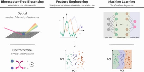
Machine Learning Enhances the Performance of Bioreceptor-Free Biosensors


Abstract
:
1. Introduction
2. How Biosensors Can Benefit from Machine Learning
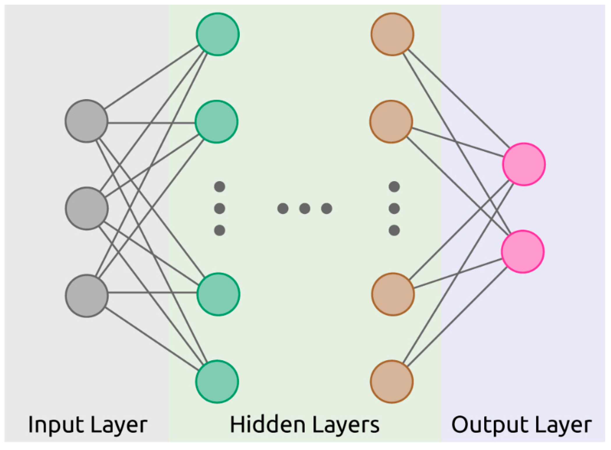
3. A Brief Tour of Machine Learning
3.1. Feature Engineering
3.2. Unsupervised vs. Supervised
3.3. Classification Algorithms
3.4. Regression Algorithms
3.5. Model Performance Assessment
4. Electrochemical Bioreceptor-Free Biosensors
4.1. Cyclic Voltammetry (CV)
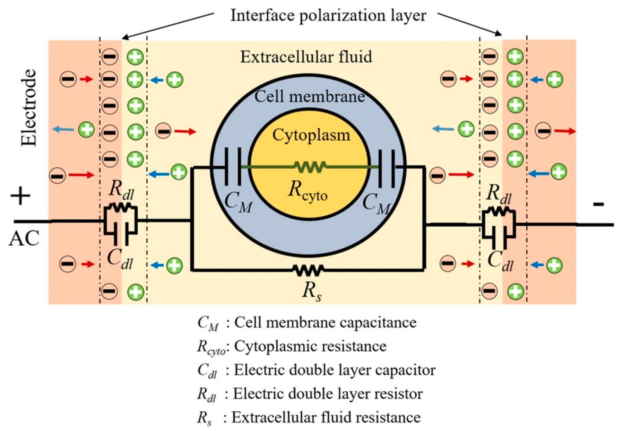
4.2. Electrical Impedance Spectroscopy (EIS)
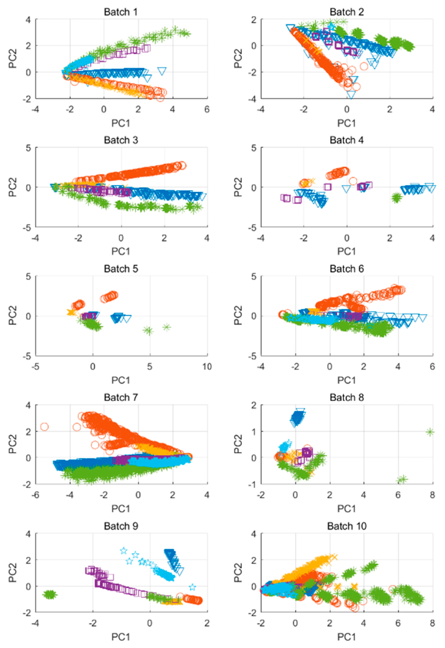
4.3. Enose and Etongue
4.4. Summary of Electrochemical Bioreceptor-Free Biosensing
5. Optical Bioreceptor-Free Biosensors
5.1. Imaging
5.2. Colorimetry
5.3. Spectroscopy
5.4. Summary of Optical Bioreceptor-Free Biosensing
6. Considerations and Future Perspectives
7. Conclusions
Author Contributions
Funding
Institutional Review Board Statement
Informed Consent Statement
Data Availability Statement
Acknowledgments
Conflicts of Interest
References
- Metkar, S.K.; Girigoswami, K. Diagnostic biosensors in medicine—A review. Biocatal. Agric. Biotechnol. 2019, 17, 271–283. [Google Scholar] [CrossRef]
- Justino, C.I.L.; Duarte, A.C.; Rocha-Santos, T.A.P. Recent progress in biosensors for environmental monitoring: A review. Sensors 2017, 17, 2918. [Google Scholar] [CrossRef] [PubMed] [Green Version]
- Nguyen, H.H.; Lee, S.H.; Lee, U.J.; Fermin, C.D.; Kim, M. Immobilized enzymes in biosensor applications. Materials 2019, 12, 121. [Google Scholar] [CrossRef] [PubMed] [Green Version]
- Hock, B. Antibodies for immunosensors a review. Anal. Chim. Acta 1997, 347, 177–186. [Google Scholar] [CrossRef]
- Lim, Y.C.; Kouzani, A.Z.; Duan, W. Aptasensors: A review. J. Biomed. Nanotechnol. 2010, 6, 93–105. [Google Scholar] [CrossRef] [PubMed]
- Massah, J.; Asefpour Vakilian, K. An intelligent portable biosensor for fast and accurate nitrate determination using cyclic voltammetry. Biosyst. Eng. 2019, 177, 49–58. [Google Scholar] [CrossRef]
- Esfahani, S.; Shanta, M.; Specht, J.P.; Xing, Y.; Cole, M.; Gardner, J.W. Wearable IoT electronic nose for urinary incontinence detection. In Proceedings of the 2020 IEEE Sensors, Virtual Conference, Rotterdam, The Netherlands, 25–28 October 2020; IEEE: Piscataway, NJ, USA, 2020; pp. 1–4. [Google Scholar] [CrossRef]
- Pelosi, P.; Zhu, J.; Knoll, W. From gas sensors to biomimetic artificial noses. Chemosensors 2018, 6, 32. [Google Scholar] [CrossRef] [Green Version]
- Wilson, A.D. Noninvasive early disease diagnosis by electronic-nose and related VOC-detection devices. Biosensors 2020, 10, 73. [Google Scholar] [CrossRef]
- Szulczyński, B.; Armiński, K.; Namieśnik, J.; Gębicki, J. Determination of odour interactions in gaseous mixtures using electronic nose methods with artificial neural networks. Sensors 2018, 18, 519. [Google Scholar] [CrossRef] [Green Version]
- Zambotti, G.; Soprani, M.; Gobbi, E.; Capuano, R.; Pasqualetti, V.; Di Natale, C.; Ponzoni, A. Early detection of fish degradation by electronic nose. In Proceedings of the 2019 IEEE International Symposium on Olfaction and Electronic Nose (ISOEN), Fukuoka, Japan, 26–29 May 2019; IEEE: Piscataway, NJ, USA, 2019; pp. 1–3. [Google Scholar] [CrossRef]
- Podrażka, M.; Bączyńska, E.; Kundys, M.; Jeleń, P.S.; Witkowska Nery, E. Electronic tongue—A tool for all tastes? Biosensors 2018, 8, 3. [Google Scholar] [CrossRef] [Green Version]
- Chen, X.; Xu, Y.; Meng, L.; Chen, X.; Yuan, L.; Cai, Q.; Shi, W.; Huang, G. Non-parametric partial least squares—Discriminant analysis model based on sum of ranking difference algorithm for tea grade identification using electronic tongue data. Sens. Actuat. B Chem. 2020, 311, 127924. [Google Scholar] [CrossRef]
- Kovacs, Z.; Szöllősi, D.; Zaukuu, J.-L.Z.; Bodor, Z.; Vitális, F.; Aouadi, B.; Zsom-Muha, V.; Gillay, Z. Factors influencing the long-term stability of electronic tongue and application of improved drift correction methods. Biosensors 2020, 10, 74. [Google Scholar] [CrossRef] [PubMed]
- Guedes, M.D.V.; Marques, M.S.; Guedes, P.C.; Contri, R.V.; Kulkamp Guerreiro, I.C. The use of electronic tongue and sensory panel on taste evaluation of pediatric medicines: A systematic review. Pharm. Dev. Technol. 2020, 26, 119–137. [Google Scholar] [CrossRef] [PubMed]
- Ross, C.F. Considerations of the use of the electronic tongue in sensory science. Curr. Opin. Food Sci. 2021, 40, 87–93. [Google Scholar] [CrossRef]
- Guerrini, L.; Alvarez-Puebla, R.A. Chapter 19—Surface-enhanced Raman scattering chemosensing of proteins. In Vibrational Spectroscopy in Protein Research; Ozaki, Y., Baranska, M., Lednev, I.K., Wood, B.R., Eds.; Academic Press: London, UK, 2020; pp. 553–567. [Google Scholar] [CrossRef]
- Feng, J.; Hu, Y.; Grant, E.; Lu, X. Determination of thiabendazole in orange juice using an MISPE-SERS chemosensor. Food Chem. 2018, 239, 816–822. [Google Scholar] [CrossRef] [Green Version]
- Langer, J.; Jimenez de Aberasturi, D.; Aizpurua, J.; Alvarez-Puebla, R.A.; Auguié, B.; Baumberg, J.J.; Bazan, G.C.; Bell, S.E.J.; Boisen, A.; Brolo, A.G.; et al. Present and future of surface-enhanced Raman scattering. ACS Nano 2020, 14, 28–117. [Google Scholar] [CrossRef] [Green Version]
- Zheng, X.S.; Jahn, I.J.; Weber, K.; Cialla-May, D.; Popp, J. Label-free SERS in biological and biomedical applications: Recent progress, current challenges and opportunities. Spectrochim. Acta A Mol. Biomol. Spectrosc. 2018, 197, 56–77. [Google Scholar] [CrossRef] [PubMed]
- Krafft, C.; Osei, E.B.; Popp, J.; Nazarenko, I. Raman and SERS spectroscopy for characterization of extracellular vesicles from control and prostate carcinoma patients. Proc. SPIE 2020, 11236, 1123602. [Google Scholar] [CrossRef]
- Sang, S.; Wang, Y.; Feng, Q.; Wei, Y.; Ji, J.; Zhang, W. Progress of new label-free techniques for biosensors: A review. Crit. Rev. Biotechnol. 2016, 36, 465–481. [Google Scholar] [CrossRef]
- Scott, S.M.; James, D.; Ali, Z. Data analysis for electronic nose systems. Microchim. Acta 2006, 156, 183–207. [Google Scholar] [CrossRef]
- Yan, J.; Guo, X.; Duan, S.; Jia, P.; Wang, L.; Peng, C.; Zhang, S. Electronic nose feature extraction methods: A review. Sensors 2015, 15, 27804–27831. [Google Scholar] [CrossRef] [PubMed]
- Hotel, O.; Poli, J.-P.; Mer-Calfati, C.; Scorsone, E.; Saada, S. A review of algorithms for SAW sensors Enose based volatile compound identification. Sens. Actuat. B Chem. 2018, 255, 2472–2482. [Google Scholar] [CrossRef]
- Da Costa, N.L.; da Costa, M.S.; Barbosa, R. A review on the application of chemometrics and machine learning algorithms to evaluate beer authentication. Food Anal. Meth. 2021, 14, 136–155. [Google Scholar] [CrossRef]
- Wasilewski, T.; Migoń, D.; Gębicki, J.; Kamysz, W. Critical review of electronic nose and tongue instruments prospects in pharmaceutical analysis. Anal. Chim. Acta 2019, 1077, 14–29. [Google Scholar] [CrossRef]
- Lussier, F.; Thibault, V.; Charron, B.; Wallace, G.Q.; Masson, J.-F. Deep learning and artificial intelligence methods for Raman and surface-enhanced Raman scattering. TrAC-Trends Anal. Chem. 2020, 124, 115796. [Google Scholar] [CrossRef]
- Cui, F.; Yue, Y.; Zhang, Y.; Zhang, Z.; Zhou, H.S. Advancing biosensors with machine learning. ACS Sens. 2020, 5, 3346–3364. [Google Scholar] [CrossRef] [PubMed]
- Sheng, Y.; Qian, W.; Huang, J.; Wu, B.; Yang, J.; Xue, T.; Ge, Y.; Wen, Y. Electrochemical detection combined with machine learning for intelligent sensing of maleic hydrazide by using carboxylated PEDOT modified with copper nanoparticles. Microchim. Acta 2019, 186, 543. [Google Scholar] [CrossRef] [PubMed]
- Dean, S.N.; Shriver-Lake, L.C.; Stenger, D.A.; Erickson, J.S.; Golden, J.P.; Trammell, S.A. Machine learning techniques for chemical identification using cyclic square wave voltammetry. Sensors 2019, 19, 2392. [Google Scholar] [CrossRef] [PubMed] [Green Version]
- Tonezzer, M.; Le, D.T.T.; Iannotta, S.; Van Hieu, N. Selective discrimination of hazardous gases using one single metal oxide resistive sensor. Sens. Actuat. B Chem. 2018, 277, 121–128. [Google Scholar] [CrossRef]
- Xu, L.; He, J.; Duan, S.; Wu, X.; Wang, Q. Comparison of machine learning algorithms for concentration detection and prediction of formaldehyde based on electronic nose. Sens. Rev. 2016, 36, 207–216. [Google Scholar] [CrossRef]
- Yang, Y.; Liu, H.; Gu, Y. A model transfer learning framework with back-propagation neural network for wine and Chinese liquor detection by electronic nose. IEEE Access 2020, 8, 105278–105285. [Google Scholar] [CrossRef]
- Leon-Medina, J.X.; Pineda-Muñoz, W.A.; Burgos, D.A.T. Joint distribution adaptation for drift correction in electronic nose type sensor arrays. IEEE Access 2020, 8, 134413–134421. [Google Scholar] [CrossRef]
- Liu, B.; Zeng, X.; Tian, F.; Zhang, S.; Zhao, L. Domain transfer broad learning system for long-term drift compensation in electronic nose systems. IEEE Access 2019, 7, 143947–143959. [Google Scholar] [CrossRef]
- Wang, X.; Gu, Y.; Liu, H. A transfer learning method for the protection of geographical indication in China using an electronic nose for the identification of Xihu Longjing tea. IEEE Sens. J. 2021, 21, 8065–8077. [Google Scholar] [CrossRef]
- Yi, R.; Yan, J.; Shi, D.; Tian, Y.; Chen, F.; Wang, Z.; Duan, S. Improving the performance of drifted/shifted electronic nose systems by cross-domain transfer using common transfer samples. Sens. Actuat. B Chem. 2021, 329, 129162. [Google Scholar] [CrossRef]
- Liang, Z.; Tian, F.; Zhang, C.; Sun, H.; Song, A.; Liu, T. Improving the robustness of prediction model by transfer learning for interference suppression of electronic nose. IEEE Sens. J. 2018, 18, 1111–1121. [Google Scholar] [CrossRef]
- Daliri, M.R. Combining extreme learning machines using support vector machines for breast tissue classification. Comput. Meth. Biomech. Biomed. Eng. 2015, 18, 185–191. [Google Scholar] [CrossRef]
- Durante, G.; Becari, W.; Lima, F.A.S.; Peres, H.E.M. Electrical impedance sensor for real-time detection of bovine milk adulteration. IEEE Sens. J. 2016, 16, 861–865. [Google Scholar] [CrossRef]
- Helwan, A.; Idoko, J.B.; Abiyev, R.H. Machine learning techniques for classification of breast tissue. Proc. Comput. Sci. 2017, 120, 402–410. [Google Scholar] [CrossRef]
- Islam, M.; Wahid, K.; Dinh, A. Assessment of ripening degree of avocado by electrical impedance spectroscopy and support vector machine. J. Food Qual. 2018, 2018, 4706147. [Google Scholar] [CrossRef] [Green Version]
- Murphy, E.K.; Mahara, A.; Khan, S.; Hyams, E.S.; Schned, A.R.; Pettus, J.; Halter, R.J. Comparative study of separation between ex vivo prostatic malignant and benign tissue using electrical impedance spectroscopy and electrical impedance tomography. Physiol. Meas. 2017, 38, 1242–1261. [Google Scholar] [CrossRef] [PubMed]
- Yang, Z.; Miao, N.; Zhang, X.; Li, Q.; Wang, Z.; Li, C.; Sun, X.; Lan, Y. Employment of an electronic tongue combined with deep learning and transfer learning for discriminating the storage time of Pu-erh tea. Food Control 2021, 121, 107608. [Google Scholar] [CrossRef]
- Leon-Medina, J.X.; Anaya, M.; Pozo, F.; Tibaduiza, D. Nonlinear feature extraction through manifold learning in an electronic tongue classification task. Sensors 2020, 20, 4834. [Google Scholar] [CrossRef]
- Giménez-Gómez, P.; Escudé-Pujol, R.; Capdevila, F.; Puig-Pujol, A.; Jiménez-Jorquera, C.; Gutiérrez-Capitán, M. Portable electronic tongue based on microsensors for the analysis of Cava wines. Sensors 2016, 16, 1796. [Google Scholar] [CrossRef] [Green Version]
- Ouyang, Q.; Yang, Y.; Wu, J.; Liu, Z.; Chen, X.; Dong, C.; Chen, Q.; Zhang, Z.; Guo, Z. Rapid sensing of total theaflavins content in black tea using a portable electronic tongue system coupled to efficient variables selection algorithms. J. Food Compos. Anal. 2019, 75, 43–48. [Google Scholar] [CrossRef]
- Li, Z.; Paul, R.; Ba Tis, T.; Saville, A.C.; Hansel, J.C.; Yu, T.; Ristaino, J.B.; Wei, Q. Non-invasive plant disease diagnostics enabled by smartphone-based fingerprinting of leaf volatiles. Nat. Plants 2019, 5, 856–866. [Google Scholar] [CrossRef]
- Tomczak, A.; Ilic, S.; Marquardt, G.; Engel, T.; Forster, F.; Navab, N.; Albarqouni, S. Multi-task multi-domain learning for digital staining and classification of leukocytes. IEEE Trans. Med. Imaging 2020. [Google Scholar] [CrossRef]
- Sagar, M.A.K.; Cheng, K.P.; Ouellette, J.N.; Williams, J.C.; Watters, J.J.; Eliceiri, K.W. Machine learning methods for fluorescence lifetime imaging (FLIM) based label-free detection of microglia. Front. Neurosci. 2020, 14, 931. [Google Scholar] [CrossRef]
- Lotfollahi, M.; Berisha, S.; Daeinejad, D.; Mayerich, D. Digital staining of high-definition Fourier transform infrared (FT-IR) images using deep learning. Appl. Spectrosc. 2019, 73, 556–564. [Google Scholar] [CrossRef]
- Rivenson, Y.; Zhang, Y.; Günaydın, H.; Teng, D.; Ozcan, A. Phase recovery and holographic image reconstruction using deep learning in neural networks. Light Sci. Appl. 2018, 7, 17141. [Google Scholar] [CrossRef]
- Rivenson, Y.; Wu, Y.; Ozcan, A. Deep learning in holography and coherent imaging. Light Sci. Appl. 2019, 8, 85. [Google Scholar] [CrossRef] [Green Version]
- Wu, Y.; Ray, A.; Wei, Q.; Feizi, A.; Tong, X.; Chen, E.; Luo, Y.; Ozcan, A. Deep learning enables high-throughput analysis of particle-aggregation-based biosensors imaged using holography. ACS Photon. 2019, 6, 294–301. [Google Scholar] [CrossRef] [Green Version]
- Wu, Y.; Calis, A.; Luo, Y.; Chen, C.; Lutton, M.; Rivenson, Y.; Lin, X.; Koydemir, H.C.; Zhang, Y.; Wang, H.; et al. Label-free bioaerosol sensing using mobile microscopy and deep learning. ACS Photon. 2018, 5, 4617–4627. [Google Scholar] [CrossRef]
- Borhani, N.; Bower, A.J.; Boppart, S.A.; Psaltis, D. Digital staining through the application of deep neural networks to multi-modal multi-photon microscopy. Biomed. Opt. Express 2019, 10, 1339–1350. [Google Scholar] [CrossRef]
- Dunker, S.; Motivans, E.; Rakosy, D.; Boho, D.; Mäder, P.; Hornick, T.; Knight, T.M. Pollen analysis using multispectral imaging flow cytometry and deep learning. New Phytol. 2021, 229, 593–606. [Google Scholar] [CrossRef]
- Rivenson, Y.; Liu, T.; Wei, Z.; Zhang, Y.; de Haan, K.; Ozcan, A. PhaseStain: The digital staining of label-free quantitative phase microscopy images using deep learning. Light Sci. Appl. 2019, 8, 23. [Google Scholar] [CrossRef] [PubMed]
- Zheng, X.; Lv, G.; Du, G.; Zhai, Z.; Mo, J.; Lv, X. Rapid and low-cost detection of thyroid dysfunction using Raman spectroscopy and an improved support vector machine. IEEE Photon. J. 2018, 10, 1–12. [Google Scholar] [CrossRef]
- Tan, A.; Zhao, Y.; Sivashanmugan, K.; Squire, K.; Wang, A.X. Quantitative TLC-SERS detection of histamine in seafood with support vector machine analysis. Food Control. 2019, 103, 111–118. [Google Scholar] [CrossRef] [Green Version]
- Chen, X.; Nguyen, T.H.D.; Gu, L.; Lin, M. Use of standing gold nanorods for detection of malachite green and crystal violet in fish by SERS. J. Food Sci. 2017, 82, 1640–1646. [Google Scholar] [CrossRef] [PubMed]
- Fornasaro, S.; Marta, S.D.; Rabusin, M.; Bonifacio, A.; Sergo, V. Toward SERS-based point-of-care approaches for therapeutic drug monitoring: The case of methotrexate. Faraday Discuss. 2016, 187, 485–499. [Google Scholar] [CrossRef] [PubMed]
- Hassoun, M.; Rüger, J.; Kirchberger-Tolstik, T.; Schie, I.W.; Henkel, T.; Weber, K.; Cialla-May, D.; Krafft, C.; Popp, J. A droplet-based microfluidic chip as a platform for leukemia cell lysate identification using surface-enhanced Raman scattering. Anal. Bioanal. Chem. 2018, 410, 999–1006. [Google Scholar] [CrossRef]
- Hidi, I.J.; Jahn, M.; Pletz, M.W.; Weber, K.; Cialla-May, D.; Popp, J. Toward levofloxacin monitoring in human urine samples by employing the LoC-SERS technique. J. Phys. Chem. C 2016, 120, 20613–20623. [Google Scholar] [CrossRef]
- Hou, M.; Huang, Y.; Ma, L.; Zhang, Z. Quantitative analysis of single and mix food antiseptics basing on SERS spectra with PLSR method. Nanoscale Res. Lett. 2016, 11, 296. [Google Scholar] [CrossRef] [Green Version]
- Kämmer, E.; Olschewski, K.; Stöckel, S.; Rösch, P.; Weber, K.; Cialla-May, D.; Bocklitz, T.; Popp, J. Quantitative SERS studies by combining LOC-SERS with the standard addition method. Anal. Bioanal. Chem. 2015, 407, 8925–8929. [Google Scholar] [CrossRef]
- Mühlig, A.; Bocklitz, T.; Labugger, I.; Dees, S.; Henk, S.; Richter, E.; Andres, S.; Merker, M.; Stöckel, S.; Weber, K.; et al. LOC-SERS: A promising closed system for the identification of mycobacteria. Anal. Chem. 2016, 88, 7998–8004. [Google Scholar] [CrossRef]
- Nguyen, C.Q.; Thrift, W.J.; Bhattacharjee, A.; Ranjbar, S.; Gallagher, T.; Darvishzadeh-Varcheie, M.; Sanderson, R.N.; Capolino, F.; Whiteson, K.; Baldi, P.; et al. Longitudinal monitoring of biofilm formation via robust surface-enhanced Raman scattering quantification of Pseudomonas aeruginosa-produced metabolites. ACS Appl. Mater. Interfaces 2018, 10, 12364–12373. [Google Scholar] [CrossRef] [PubMed]
- Othman, N.H.; Lee, K.Y.; Radzol, A.R.M.; Mansor, W. PCA-SCG-ANN for detection of non-structural protein 1 from SERS salivary spectra. In Intelligent Information and Database Systems; Nguyen, N.T., Tojo, S., Nguyen, L.M., Trawiński, B., Eds.; Springer: Cham, Switzerland, 2017; pp. 424–433. [Google Scholar] [CrossRef]
- Othman, N.H.; Yoot Lee, K.; Mohd Radzol, A.R.; Mansor, W.; Amanina Yusoff, N. PCA-polynomial-ELM model optimal for detection of NS1 adulterated salivary SERS spectra. J. Phys. Conf. Ser. 2019, 1372, 012064. [Google Scholar] [CrossRef]
- Seifert, S.; Merk, V.; Kneipp, J. Identification of aqueous pollen extracts using surface enhanced Raman scattering (SERS) and pattern recognition methods. J. Biophotonics 2016, 9, 181–189. [Google Scholar] [CrossRef]
- Sun, H.; Lv, G.; Mo, J.; Lv, X.; Du, G.; Liu, Y. Application of KPCA combined with SVM in Raman spectral discrimination. Optik 2019, 184, 214–219. [Google Scholar] [CrossRef]
- Wold, S.; Esbensen, K.; Geladi, P. Principal component analysis. Chemom. Intell. Lab. Syst. 1987, 2, 37–52. [Google Scholar] [CrossRef]
- Cunningham, P. Dimension reduction. In Machine Learning Techniques for Multimedia: Case Studies on Organization and Retrieval, Cognitive Technologies; Cord, M., Cunningham, P., Eds.; Springer: Berlin/Heidelberg, Germany, 2008; pp. 91–112. [Google Scholar] [CrossRef]
- Alpaydin, E. Introduction to Machine Learning; MIT Press: Cambridge, MA, USA, 2020. [Google Scholar]
- Peterson, L.E. K-nearest neighbor. Scholarpedia 2009, 4, 1883. [Google Scholar] [CrossRef]
- Balaprakash, P.; Salim, M.; Uram, T.D.; Vishwanath, V.; Wild, S.M. DeepHyper: Asynchronous hyperparameter search for deep neural networks. In Proceedings of the 2018 IEEE 25th International Conference on High Performance Computing (HiPC), Bengaluru, India, 17–20 December 2018; IEEE: Piscataway, NJ, USA, 2019; pp. 42–51. [Google Scholar] [CrossRef]
- Boser, B.E.; Guyon, I.M.; Vapnik, V.N. A training algorithm for optimal margin classifiers. In Proceedings of the Fifth Annual Workshop on Computational Learning Theory, COLT’92, Pittsburgh, PA, USA, 27–29 July 1992; Association for Computing Machinery: New York, NY, USA, 1992; pp. 144–152. [Google Scholar] [CrossRef]
- Zhang, J. A complete list of kernels used in support vector machines. Biochem. Pharmacol. 2015, 4, 2. [Google Scholar] [CrossRef] [Green Version]
- Mathur, A.; Foody, G.M. Multiclass and binary SVM classification: Implications for training and classification users. IEEE Geosci. Remote Sens. Lett. 2008, 5, 241–245. [Google Scholar] [CrossRef]
- Shawe-Taylor, J.; Cristianini, N. On the generalization of soft margin algorithms. IEEE Trans. Inf. Theory 2002, 48, 2721–2735. [Google Scholar] [CrossRef]
- Han, H.; Jiang, X. Overcome support vector machine diagnosis overfitting. Cancer Inform. 2014, 13, 145–158. [Google Scholar] [CrossRef]
- Ghojogh, B.; Crowley, M. Linear and quadratic discriminant analysis: Tutorial. arXiv 2019, arXiv:1906.02590. Available online: https://arxiv.org/abs/1906.02590v1 (accessed on 2 August 2021).
- Myles, A.J.; Feudale, R.N.; Liu, Y.; Woody, N.A.; Brown, S.D. An introduction to decision tree modeling. J. Chemom. 2004, 18, 275–285. [Google Scholar] [CrossRef]
- Lewis, R.J. An introduction to classification and regression tree (CART) analysis. In The 2000 Annual Meeting of the Society for Academic Emergency Medicine in San Francisco, California; Society for Academic Emergency Medicine: Des Plaines, IL, USA, 2000; Available online: http://citeseerx.ist.psu.edu/viewdoc/download?doi=10.1.1.95.4103&rep=rep1&type=pdf (accessed on 4 August 2021).
- Criminisi, A.; Shotton, J.; Konukoglu, E. Decision forests: A unified framework for classification, regression, density estimation, manifold learning and semi-supervised learning. Found. Trends Comput. Graph. Vis. 2012, 7, 81–227. [Google Scholar] [CrossRef]
- Sherstinsky, A. Fundamentals of recurrent neural network (RNN) and long short-term memory (LSTM) network. Phys. D Nonlinear Phenom. 2020, 404, 132306. [Google Scholar] [CrossRef] [Green Version]
- Huang, G.B.; Zhu, Q.Y.; Siew, C.-K. Extreme learning machine: Theory and applications. Neurocomput. Neural Netw. 2006, 70, 489–501. [Google Scholar] [CrossRef]
- Fukushima, K. Neocognitron: A hierarchical neural network capable of visual pattern recognition. Neural Netw. 1998, 1, 119–130. [Google Scholar] [CrossRef]
- Hinton, G.E.; Salakhutdinov, R.R. Reducing the dimensionality of data with neural networks. Science 2006, 313, 504–507. [Google Scholar] [CrossRef] [Green Version]
- Hecht-Nielsen, R. Theory of the backpropagation neural network. In Neural Networks for Perception, Volume 2: Computation, Learning, and Architectures; Academic Press: Boston, MA, USA, 1992; pp. 65–93. [Google Scholar] [CrossRef]
- Alto, V. Neural Networks: Parameters, Hyperparameters and Optimization Strategies. Available online: https://towardsdatascience.com/neural-networks-parameters-hyperparameters-and-optimization-strategies-3f0842fac0a5 (accessed on 2 August 2021).
- Goodfellow, I.J.; Pouget-Abadie, J.; Mirza, M.; Xu, B.; Warde-Farley, D.; Ozair, S.; Courville, A.; Bengio, Y. Generative adversarial networks. arXiv 2014, arXiv:1406.2661. Available online: https://arxiv.org/abs/1406.2661 (accessed on 13 April 2021). [CrossRef]
- Zhang, F.; O’Donnell, L.J. Chapter 7—Support vector regression. In Machine Learning; Mechelli, A., Vieira, S., Eds.; Academic Press: London, UK, 2020; pp. 123–140. [Google Scholar] [CrossRef]
- Hoffmann, F.; Bertram, T.; Mikut, R.; Reischl, M.; Nelles, O. Benchmarking in classification and regression. WIREs 2019, 9, e1318. [Google Scholar] [CrossRef]
- Shao, J. Linear model selection by cross-validation. J. Am. Stat. Assoc. 1993, 88, 486–494. [Google Scholar] [CrossRef]
- Yoon, J.-Y. Introduction to Biosensors: From Electric Circuits to Immunosensors, 2nd ed.; Springer: New York, NY, USA, 2016. [Google Scholar] [CrossRef]
- Grieshaber, D.; MacKenzie, R.; Vörös, J.; Reimhult, E. Electrochemical biosensors—Sensor principles and architectures. Sensors 2008, 8, 1400–1458. [Google Scholar] [CrossRef] [PubMed]
- Dhanjai; Sinha, A.; Lu, X.; Wu, L.; Tan, D.; Li, Y.; Chen, J.; Jain, R. Voltammetric sensing of biomolecules at carbon based electrode interfaces: A review. TrAC—Trends Anal. Chem. 2018, 98, 174–189. [Google Scholar] [CrossRef]
- Grossi, M.; Riccò, B. Electrical impedance spectroscopy (EIS) for biological analysis and food characterization: A review. J. Sens. Sens. Syst. 2017, 6, 303–325. [Google Scholar] [CrossRef] [Green Version]
- Yao, J.; Wang, L.; Liu, K.; Wu, H.; Wang, H.; Huang, J.; Li, J. Evaluation of electrical characteristics of biological tissue with electrical impedance spectroscopy. Electrophoresis 2020, 41, 1425–1432. [Google Scholar] [CrossRef]
- Jossinet, J. Variability of impedivity in normal and pathological breast tissue. Med. Biol. Eng. Comput. 1996, 34, 346–350. [Google Scholar] [CrossRef]
- Dua, D.; Graff, C. UCI Machine Learning Repository (https://archive.ics.uci.edu/); University of California, Irvine, School of Information and Computer Sciences: Irvine, CA, USA, 2017. [Google Scholar]
- Estrela da Silva, J.; Marques de Sá, J.P.; Jossinet, J. Classification of breast tissue by electrical impedance spectroscopy. Med. Biol. Eng. Comput. 2000, 38, 26–30. [Google Scholar] [CrossRef]
- Wasilewski, T.; Kamysz, W.; Gębicki, J. Bioelectronic tongue: Current status and perspectives. Biosens. Bioelectron. 2020, 150, 111923. [Google Scholar] [CrossRef] [PubMed]
- Röck, F.; Barsan, N.; Weimar, U. Electronic nose: Current status and future trends. Chem. Rev. 2008, 108, 705–725. [Google Scholar] [CrossRef] [PubMed]
- Ha, D.; Sun, Q.; Su, K.; Wan, H.; Li, H.; Xu, N.; Sun, F.; Zhuang, L.; Hu, N.; Wang, P. Recent achievements in electronic tongue and bioelectronic tongue as taste sensors. Sens. Actuat. B: Chem. 2015, 207, 1136–1146. [Google Scholar] [CrossRef]
- Chen, C.Y.; Lin, W.C.; Yang, H.Y. Diagnosis of ventilator-associated pneumonia using electronic nose sensor array signals: Solutions to improve the application of machine learning in respiratory research. Respir. Res. 2020, 21, 45. [Google Scholar] [CrossRef]
- Tan, J.; Xu, J. Applications of electronic nose (Enose) and electronic tongue (Etongue) in food quality-related properties determination: A review. Artif. Intell. Agric. 2020, 4, 104–115. [Google Scholar] [CrossRef]
- Sanaeifar, A.; ZakiDizaji, H.; Jafari, A.; de la Guardia, M. Early detection of contamination and defect in foodstuffs by electronic nose: A review. TrAC—Trends Anal. Chem. 2017, 97, 257–271. [Google Scholar] [CrossRef]
- Zhang, L.; Tian, F.; Kadri, C.; Xiao, B.; Li, H.; Pan, L.; Zhou, H. On-line sensor calibration transfer among electronic nose instruments for monitoring volatile organic chemicals in indoor air quality. Sens. Actuat. B Chem. 2011, 160, 899–909. [Google Scholar] [CrossRef]
- Ciosek, P.; Wróblewski, W. Sensor arrays for liquid sensing—Electronic tongue systems. Analyst 2007, 132, 963–978. [Google Scholar] [CrossRef]
- Liu, H.; Li, Q.; Li, Z.; Gu, Y. A suppression method of concentration background noise by transductive transfer learning for a metal oxide semiconductor-based electronic nose. Sensors 2020, 20, 1913. [Google Scholar] [CrossRef] [Green Version]
- Vergara, A.; Vembu, S.; Ayhan, T.; Ryan, M.A.; Homer, M.L.; Huerta, R. Chemical gas sensor drift compensation using classifier ensembles. Sens. Actuat. B Chem. 2012, 166–167, 320–329. [Google Scholar] [CrossRef]
- Zhang, L.; Tian, F.; Peng, X.; Dang, L.; Li, G.; Liu, S.; Kadri, C. Standardization of metal oxide sensor array using artificial neural networks through experimental design. Sens. Actuat. B Chem. 2013, 177, 947–955. [Google Scholar] [CrossRef]
- DeVere, R. Disorders of taste and smell. Continuum 2017, 23, 421. [Google Scholar] [CrossRef]
- Biancolillo, A.; Boqué, R.; Cocchi, M.; Marini, F. Chapter 10—Data fusion strategies in food analysis. In Data Handling in Science and Technology; Cocchi, M., Ed.; Elsevier: Amsterdam, The Netherlands, 2019; Volume 31, pp. 271–310. [Google Scholar] [CrossRef]
- Banerjee, M.B.; Roy, R.B.; Tudu, B.; Bandyopadhyay, R.; Bhattacharyya, N. Black tea classification employing feature fusion of E-nose and E-tongue responses. J. Food Eng. 2019, 244, 55–63. [Google Scholar] [CrossRef]
- Men, H.; Shi, Y.; Fu, S.; Jiao, Y.; Qiao, Y.; Liu, J. Mining feature of data fusion in the classification of beer flavor information using E-tongue and E-nose. Sensors 2017, 17, 1656. [Google Scholar] [CrossRef] [PubMed] [Green Version]
- Buratti, S.; Malegori, C.; Benedetti, S.; Oliveri, P.; Giovanelli, G. E-nose, E-tongue and E-eye for edible olive oil characterization and shelf life assessment: A powerful data fusion approach. Talanta 2018, 182, 131–141. [Google Scholar] [CrossRef]
- Dai, C.; Huang, X.; Huang, D.; Lv, R.; Sun, J.; Zhang, Z.; Ma, M.; Aheto, J.H. Detection of submerged fermentation of Tremella aurantialba using data fusion of electronic nose and tongue. J. Food Proc. Eng. 2019, 42, e13002. [Google Scholar] [CrossRef]
- Tian, X.; Wang, J.; Ma, Z.; Li, M.; Wei, Z. Combination of an E-nose and an E-tongue for adulteration detection of minced mutton mixed with pork. J. Food Qual. 2019, 2019, e4342509. [Google Scholar] [CrossRef] [Green Version]
- Di Rosa, A.R.; Leone, F.; Cheli, F.; Chiofalo, V. Fusion of electronic nose, electronic tongue and computer vision for animal source food authentication and quality assessment—A review. J. Food Eng. 2017, 210, 62–75. [Google Scholar] [CrossRef]
- Cave, J.W.; Wickiser, J.K.; Mitropoulos, A.N. Progress in the development of olfactory-based bioelectronic chemosensors. Biosens. Bioelectron. 2019, 123, 211–222. [Google Scholar] [CrossRef]
- Ahn, S.R.; An, J.H.; Song, H.S.; Park, J.W.; Lee, S.H.; Kim, J.H.; Jang, J.; Park, T.H. Duplex bioelectronic tongue for sensing umami and sweet tastes based on human taste receptor nanovesicles. ACS Nano 2016, 10, 7287–7296. [Google Scholar] [CrossRef] [PubMed]
- Edachana, R.P.; Kumaresan, A.; Balasubramanian, V.; Thiagarajan, R.; Nair, B.G.; Thekkedath Gopalakrishnan, S.B. Paper-based device for the colorimetric assay of bilirubin based on in-vivo formation of gold nanoparticles. Microchim. Acta 2019, 187, 60. [Google Scholar] [CrossRef]
- Mutlu, A.Y.; Kılıç, V.; Kocakuşak Özdemir, G.; Bayram, A.; Horzum, N.; Solmaz, M.E. Smartphone-based colorimetric detection via machine learning. Analyst 2017, 142, 2434–2441. [Google Scholar] [CrossRef] [Green Version]
- Solmaz, M.E.; Mutlu, A.Y.; Alankus, G.; Kılıç, V.; Bayram, A.; Horzum, N. Quantifying colorimetric tests using a smartphone app based on machine learning classifiers. Sens. Actuat. B Chem. 2018, 255, 1967–1973. [Google Scholar] [CrossRef]
- Lin, B.; Yu, Y.; Cao, Y.; Guo, M.; Zhu, D.; Dai, J.; Zheng, M. Point-of-care testing for streptomycin based on aptamer recognizing and digital image colorimetry by smartphone. Biosens. Bioelectron. 2018, 100, 482–489. [Google Scholar] [CrossRef] [PubMed]
- Song, E.; Yu, M.; Wang, Y.; Hu, W.; Cheng, D.; Swihart, M.T.; Song, Y. Multi-color quantum dot-based fluorescence immunoassay array for simultaneous visual detection of multiple antibiotic residues in milk. Biosens. Bioelectron. 2015, 72, 320–325. [Google Scholar] [CrossRef] [PubMed]
- Wang, L.; Chen, W.; Ma, W.; Liu, L.; Ma, W.; Zhao, Y.; Zhu, Y.; Xu, L.; Kuang, H.; Xu, C. Fluorescent strip sensor for rapid determination of toxins. Chem. Commun. 2011, 47, 1574–1576. [Google Scholar] [CrossRef] [PubMed]
- Chen, X.; Lan, J.; Liu, Y.; Li, L.; Yan, L.; Xia, Y.; Wu, F.; Li, C.; Li, S.; Chen, J. A paper-supported aptasensor based on upconversion luminescence resonance energy transfer for the accessible determination of exosomes. Biosens. Bioelectron. 2018, 102, 582–588. [Google Scholar] [CrossRef] [PubMed]
- Guo, X. Surface plasmon resonance based biosensor technique: A review. J. Biophoton. 2012, 5, 483–501. [Google Scholar] [CrossRef] [PubMed]
- Heinze, B.C.; Yoon, J.-Y. Nanoparticle immunoagglutination Rayleigh scatter assay to complement microparticle immunoagglutination Mie scatter assay in a microfluidic device. Colloids Surf. B Biointerfaces 2011, 85, 168–173. [Google Scholar] [CrossRef]
- Park, T.S.; Li, W.; McCracken, K.E.; Yoon, J.-Y. Smartphone quantifies Salmonella from paper microfluidics. Lab Chip 2013, 13, 4832–4840. [Google Scholar] [CrossRef] [PubMed]
- Elad, T.; Benovich, E.; Magrisso, S.; Belkin, S. Toxicant identification by a luminescent bacterial bioreporter panel: Application of pattern classification algorithms. Environ. Sci. Technol. 2008, 42, 8486–8491. [Google Scholar] [CrossRef]
- Jouanneau, S.; Durand, M.-J.; Courcoux, P.; Blusseau, T.; Thouand, G. Improvement of the identification of four heavy metals in environmental samples by using predictive decision tree models coupled with a set of five bioluminescent bacteria. Environ. Sci. Technol. 2011, 45, 2925–2931. [Google Scholar] [CrossRef] [PubMed]
- Gou, T.; Hu, J.; Zhou, S.; Wu, W.; Fang, W.; Sun, J.; Hu, Z.; Shen, H.; Mu, Y. A new method using machine learning for automated image analysis applied to chip-based digital assays. Analyst 2019, 144, 3274–3281. [Google Scholar] [CrossRef] [PubMed]
- Ker, J.; Wang, L.; Rao, J.; Lim, T. Deep learning applications in medical image analysis. IEEE Access 2018, 6, 9375–9389. [Google Scholar] [CrossRef]
- Uslu, F.; Icoz, K.; Tasdemir, K.; Yilmaz, B. Automated quantification of immunomagnetic beads and leukemia cells from optical microscope images. Biomed. Signal Proc. Control. 2019, 49, 473–482. [Google Scholar] [CrossRef]
- Zeng, N.; Wang, Z.; Zhang, H.; Liu, W.; Alsaadi, F.E. Deep belief networks for quantitative analysis of a gold immunochromatographic strip. Cogn. Comput. 2016, 8, 684–692. [Google Scholar] [CrossRef] [Green Version]
- Roy, M.; Seo, D.; Oh, S.; Yang, J.-W.; Seo, S. A review of recent progress in lens-free imaging and sensing. Biosens. Bioelectron. 2017, 88, 130–143. [Google Scholar] [CrossRef]
- Wu, Y.; Ozcan, A. Lensless digital holographic microscopy and its applications in biomedicine and environmental monitoring. Methods 2018, 136, 4–16. [Google Scholar] [CrossRef]
- Greenbaum, A.; Luo, W.; Su, T.W.; Göröcs, Z.; Xue, L.; Isikman, S.O.; Coskun, A.F.; Mudanyali, O.; Ozcan, A. Imaging without lenses: Achievements and remaining challenges of wide-field on-chip microscopy. Nat. Methods 2012, 9, 889–895. [Google Scholar] [CrossRef]
- Slaoui, M.; Fiette, L. Histopathology procedures: From tissue sampling to histopathological evaluation. In Drug Safety Evaluation: Methods and Protocols; Gautier, J.-C., Ed.; Humana Press: Totowa, NJ, USA, 2011; pp. 69–82. [Google Scholar] [CrossRef]
- Yi, X.; Walia, E.; Babyn, P. Generative adversarial network in medical imaging: A review. Med. Image Anal. 2019, 58, 101552. [Google Scholar] [CrossRef] [Green Version]
- Rana, A.; Yauney, G.; Lowe, A.; Shah, P. Computational histological staining and destaining of prostate core biopsy RGB images with generative adversarial neural networks. In 2018 17th IEEE International Conference on Machine Learning and Applications (ICMLA); IEEE: Piscataway, NJ, USA, 2018; pp. 828–834. [Google Scholar] [CrossRef] [Green Version]
- Affonso, C.; Rossi, A.L.D.; Vieira, F.H.A.; de Leon Ferreira de Carvalho, A.C.P. Deep learning for biological image classification. Expert Syst. Appl. 2017, 85, 114–122. [Google Scholar] [CrossRef] [Green Version]
- Russakovsky, O.; Deng, J.; Su, H.; Krause, J.; Satheesh, S.; Ma, S.; Huang, Z.; Karpathy, A.; Khosla, A.; Bernstein, M.; et al. ImageNet large scale visual recognition challenge. Int. J. Comput. Vis. 2015, 115, 211–252. [Google Scholar] [CrossRef] [Green Version]
- Yang, T.; Guo, X.; Wang, H.; Fu, S.; Wen, Y.; Yang, H. Magnetically optimized SERS assay for rapid detection of trace drug-related biomarkers in saliva and fingerprints. Biosens. Bioelectron. 2015, 68, 350–357. [Google Scholar] [CrossRef]
- Zhang, D.; Huang, L.; Liu, B.; Ni, H.; Sun, L.; Su, E.; Chen, H.; Gu, Z.; Zhao, X. Quantitative and ultrasensitive detection of multiplex cardiac biomarkers in lateral flow assay with core-shell SERS nanotags. Biosens. Bioelectron. 2018, 106, 204–211. [Google Scholar] [CrossRef] [PubMed]
- Schlücker, S. Surface-enhanced Raman spectroscopy: Concepts and chemical applications. Angew. Chem. Int. Ed. 2014, 53, 4756–4795. [Google Scholar] [CrossRef]
- Chen, Y.; Zhang, Y.; Pan, F.; Liu, J.; Wang, K.; Zhang, C.; Cheng, S.; Lu, L.; Zhang, W.; Zhang, Z.; et al. Breath analysis based on surface-enhanced Raman scattering sensors distinguishes early and advanced gastric cancer patients from healthy persons. ACS Nano 2016, 10, 8169–8179. [Google Scholar] [CrossRef]
- Banaei, N.; Moshfegh, J.; Mohseni-Kabir, A.; Houghton, J.M.; Sun, Y.; Kim, B. Machine learning algorithms enhance the specificity of cancer biomarker detection using SERS-based immunoassays in microfluidic chips. RSC Adv. 2019, 9, 1859–1868. [Google Scholar] [CrossRef] [Green Version]
- Guselnikova, O.; Postnikov, P.; Pershina, A.; Svorcik, V.; Lyutakov, O. Express and portable label-free DNA detection and recognition with SERS platform based on functional Au grating. Appl. Surf. Sci. 2019, 470, 219–227. [Google Scholar] [CrossRef]
- Goodacre, R.; Graham, D.; Faulds, K. Recent developments in quantitative SERS: Moving towards absolute quantification. TrAC—Trends Anal. Chem. 2018, 102, 359–368. [Google Scholar] [CrossRef] [Green Version]
- Guselnikova, O.; Trelin, A.; Skvortsova, A.; Ulbrich, P.; Postnikov, P.; Pershina, A.; Sykora, D.; Svorcik, V.; Lyutakov, O. Label-free surface-enhanced Raman spectroscopy with artificial neural network technique for recognition photoinduced DNA damage. Biosens. Bioelectron. 2019, 145, 111718. [Google Scholar] [CrossRef] [PubMed]
- Thrift, W.J.; Cabuslay, A.; Laird, A.B.; Ranjbar, S.; Hochbaum, A.I.; Ragan, R. Surface-enhanced Raman scattering-based odor compass: Locating multiple chemical sources and pathogens. ACS Sens. 2019, 4, 2311–2319. [Google Scholar] [CrossRef] [PubMed]
- Thrift, W.J.; Nguyen, C.Q.; Wang, J.; Kahn, J.E.; Dong, R.; Laird, A.B.; Ragan, R. Improved regressions with convolutional neural networks for surface enhanced Raman scattering sensing of metabolite biomarkers. Proc. SPIE 2019, 11089, 1108907. [Google Scholar] [CrossRef]
- Thrift, W.J.; Ragan, R. Quantification of analyte concentration in the single molecule regime using convolutional neural networks. Anal. Chem. 2019, 91, 13337–13342. [Google Scholar] [CrossRef] [Green Version]
- Cheng, L.; Meng, Q.H.; Lilienthal, A.J.; Qi, P.F. Development of compact electronic noses: A review. Meas. Sci. Technol. 2021, 32, 062002. [Google Scholar] [CrossRef]
- Jiang, L.; Hassan, M.M.; Ali, S.; Li, H.; Sheng, R.; Chen, Q. Evolving trends in SERS-based techniques for food quality and safety: A review. Trends Food Sci. Technol. 2021, 112, 225–240. [Google Scholar] [CrossRef]
- Pang, S.; Yang, T.; He, L. Review of surface enhanced Raman spectroscopic (SERS) detection of synthetic chemical pesticides. TrAC—Trends Anal. Chem. 2016, 85, 73–82. [Google Scholar] [CrossRef] [Green Version]
- Barreiros dos Santos, M.; Queirós, R.B.; Geraldes, Á.; Marques, C.; Vilas-Boas, V.; Dieguez, L.; Paz, E.; Ferreira, R.; Morais, J.; Vasconcelos, V.; et al. Portable sensing system based on electrochemical impedance spectroscopy for the simultaneous quantification of free and total microcystin-LR in freshwaters. Biosens. Bioelectron. 2019, 142, 111550. [Google Scholar] [CrossRef]
- Huang, X.; Li, Y.; Xu, X.; Wang, R.; Yao, J.; Han, W.; Wei, M.; Chen, J.; Xuan, W.; Sun, L. High-precision lensless microscope on a chip based on in-line holographic imaging. Sensors 2021, 21, 720. [Google Scholar] [CrossRef]
- Zhang, R.; Belwal, T.; Li, L.; Lin, X.; Xu, Y.; Luo, Z. Nanomaterial-based biosensors for sensing key foodborne pathogens: Advances from recent decades. Compr. Rev. Food Sci. Food Saf. 2020, 19, 1465–1487. [Google Scholar] [CrossRef]
- Wang, Q.; Wei, H.; Zhang, Z.; Wang, E.; Dong, S. Nanozyme: An emerging alternative to natural enzyme for biosensing and immunoassay. TrAC—Trends Anal. Chem. 2018, 105, 218–224. [Google Scholar] [CrossRef]
- Zhu, X.; Liu, P.; Ge, Y.; Wu, R.; Xue, T.; Sheng, Y.; Ai, S.; Tang, K.; Wen, Y. MoS2/MWCNTs porous nanohybrid network with oxidase-like characteristic as electrochemical nanozyme sensor coupled with machine learning for intelligent analysis of carbendazim. J. Electroanal. Chem. 2020, 862, 113940. [Google Scholar] [CrossRef]
- Mahmudunnabi, G.R.; Farhana, F.Z.; Kashaninejad, N.; Firoz, S.H.; Shim, Y.-B.; Shiddiky, M.J.A. Nanozyme-based electrochemical biosensors for disease biomarker detection. Analyst 2020, 145, 4398–4420. [Google Scholar] [CrossRef]
- Zhang, X.; Wu, D.; Zhou, X.; Yu, Y.; Liu, J.; Hu, N.; Wang, H.; Li, G.; Wu, Y. Recent progress in the construction of nanozyme-based biosensors and their applications to food safety assay. TrAC—Trends Anal. Chem. 2019, 121, 115668. [Google Scholar] [CrossRef]
- Riley, P. Three pitfalls to avoid in machine learning. Nature 2019, 572, 27–29. [Google Scholar] [CrossRef] [PubMed] [Green Version]
- Stodden, V.; McNutt, M.; Bailey, D.H.; Deelman, E.; Gil, Y.; Hanson, B.; Heroux, M.A.; Ioannidis, J.P.A.; Taufer, M. Enhancing reproducibility for computational methods. Science 2016, 354, 1240–1241. [Google Scholar] [CrossRef] [PubMed]


| Biosensing Mechanism | Task | Target | Algorithm | Ref. |
|---|---|---|---|---|
| ELECTROCHEMICAL | ||||
| CV | Regression | Maleic hydrazide | ANN | [30] |
| CV | Classification | Industrial chemicals | LSTM, CNN | [31] |
| Enose | Feature extraction | Harmful gases | PCA | [32] |
| Classification | DT, RF, SVM | |||
| Regression | SVR | |||
| Enose | Regression | Formaldehyde | BPNN | [33] |
| Enose | Classification | Chinese wines | BPNN | [34] |
| Target task change | Chinese liquors | Transfer learning | ||
| Enose | Sensor drift compensation for classification | Gases | JDA | [35] |
| DTBLS | [36] | |||
| TrLightGBM | [37] | |||
| ELM | [38] | |||
| Enose | Sensor drift compensation & noise reduction | Bacteria | ELM | [39] |
| EIS | Classification | Breast tissue | ELM + SVM | [40] |
| EIS | Classification | Milk adulteration | k-NN | [41] |
| EIS | Classification | Breast tissue | RBFN | [42] |
| EIS | Feature extraction | Avocado ripeness | PCA | [43] |
| Classification | SVM | |||
| EIS & EIT | Classification | Prostatic tissue | SVM | [44] |
| Etongue | Taste classification | Tea storage time | CNN | [45] |
| Increase generalizability | Transfer learning | |||
| Etongue | Feature Extraction | Beverages | t-SNE | [46] |
| Classification | k-NN | |||
| Etongue | Classification | Cava wine age | LDA | [47] |
| Etongue | Regression | Black tea theaflavin | Si-CARS-PLS | [48] |
| OPTICAL | ||||
| Colorimetric | Classification | Plant disease VOCs (blight) | PCA | [49] |
| Diff. contrast microscopy | Digital staining & domain adaptation | Leukocytes | GAN | [50] |
| Fluorescence imaging | Classification | Microglia | ANN | [51] |
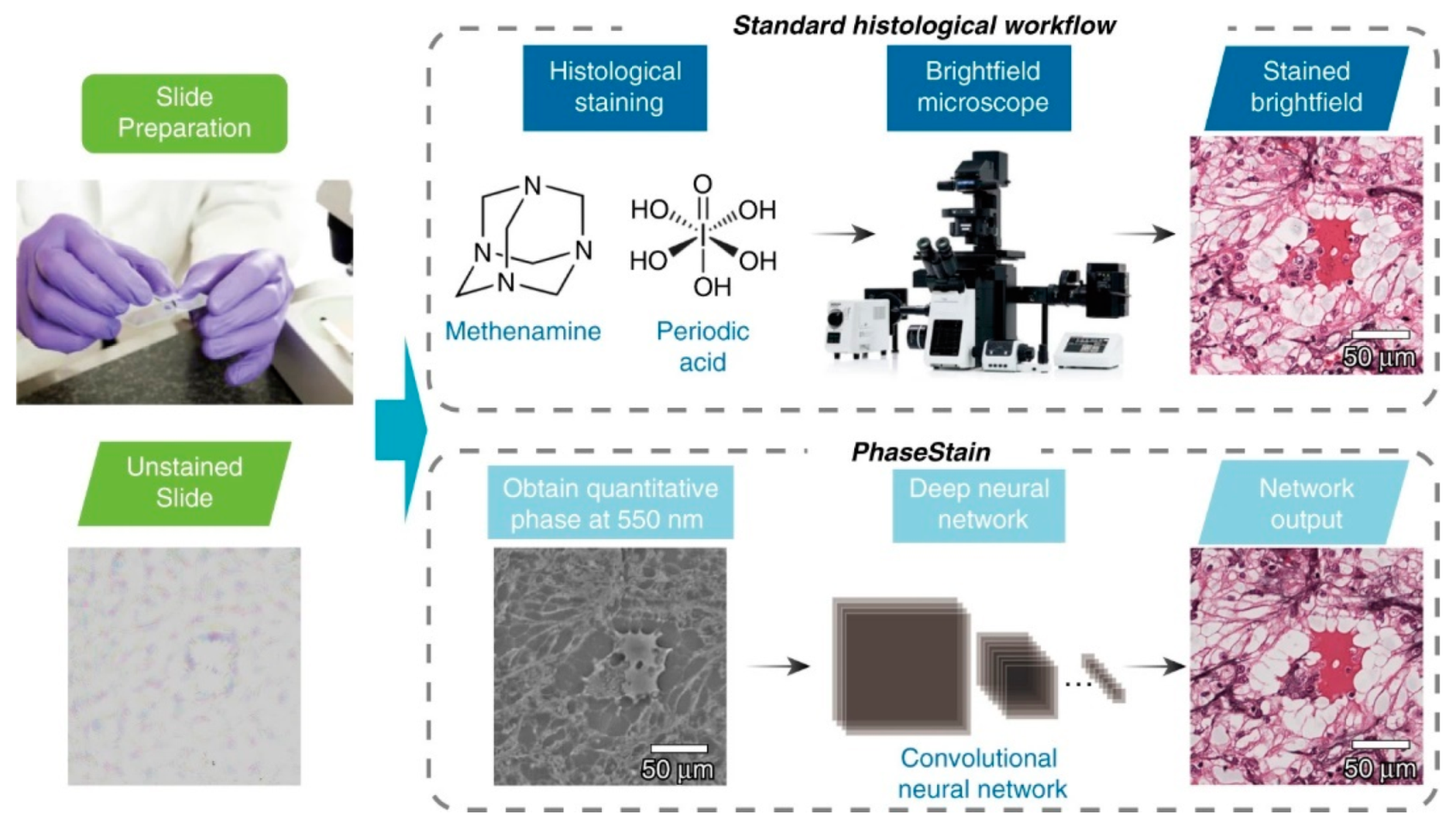
| FTIR imaging | Digital staining | H&E stain | Deep CNN | [52] |
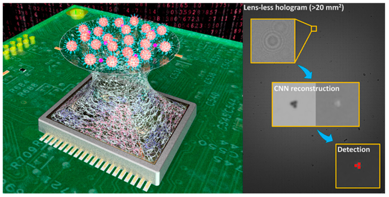
| Lens-free imaging | Image reconstruction | Blood & tissue | CNN | [53,54] |
| Herpes | [55] | |||
| Lens-free imaging | Image reconstruction & classification | Bioaerosol | CNN | [56] |
| Multi-modal multi-photon microscopy | Digital staining & modal mapping | Liver tissue | DNN | [57] |
| Multispectral imaging | Classification | Pollen species | CNN | [58] |
| Quantitative phase imaging | Digital staining | Skin, kidney & liver tissue | GAN | [59] |
| Raman spectroscopy | Feature extraction | Thyroid dysfunction biomarker | PCA | [60] |
| Classification | SVM | |||
| TLC-SERS | Feature extraction | Histamine | PCA | [61] |
| Quantification | SVR | |||
| SERS | Exploratory analysis | Malachite green & crystal violet | PCA | [37,62] |
| Quantification | PLSR | |||
| SERS | Quantification | Methotrexate | PLSR | [63] |
| SERS | Classification | Oil vs lysate spectra Leukemia cell lysate | k-means clustering | [64] |
| Dimension reduction | PCA | |||
| Classification | SVM | |||
| SERS | Dimension reduction | Levofloxacin | PCA | [38,65] |
| Regression | PLSR | |||
| SERS | Quantification | Potassium sorbate & sodium benzoate | PLSR | [66] |
| SERS | Dimension reduction & regression | Congo red | PCR | [39,67] |
| SERS | Dimension reduction | Mycobacteria | PCA | [40,68] |
| Classification | LDA | |||
| SERS | Quantification | Biofilm formation | PLSR | [41,69] |
| SERS | Feature extraction | Non-structural protein 1 | PCA | [70,71] |
| Classification | BPNN, ELM | |||
| SERS | Exploratory analysis | Pollen species | PCA, HCA | [72] |
| Classification | ANN | |||
| SERS | Feature extraction | Human serum | KPCA | [73] |
| Classification | SVM | |||
| Biosensing Mechanism | Description of Data | Feature Extraction | ML Model |
|---|---|---|---|
| CV | Cyclic voltammogram | ANN, LSTM, CNN | |
| EIS | Nyquist plot | PCA | k-NN, ELM, SVM, RBFN |
| Enose | Multivariate | PCA | DT, RF, ELM, SVM, BPNN |
| Etongue | Multivariate | PCA, t-SNE | LDA, k-NN, CNN, PLS |
| Lens-free imaging | Image | CNN | |
| Digital staining | Image | Deep learning, GAN | |
| SERS | Spectrum | PCA, KPCA | PLSR, LDA, SVM, SVR, BPNN, ELM |
Publisher’s Note: MDPI stays neutral with regard to jurisdictional claims in published maps and institutional affiliations. |
© 2021 by the authors. Licensee MDPI, Basel, Switzerland. This article is an open access article distributed under the terms and conditions of the Creative Commons Attribution (CC BY) license (https://creativecommons.org/licenses/by/4.0/).
Share and Cite
Schackart, K.E., III; Yoon, J.-Y. Machine Learning Enhances the Performance of Bioreceptor-Free Biosensors. Sensors 2021, 21, 5519. https://doi.org/10.3390/s21165519
Schackart KE III, Yoon J-Y. Machine Learning Enhances the Performance of Bioreceptor-Free Biosensors. Sensors. 2021; 21(16):5519. https://doi.org/10.3390/s21165519
Chicago/Turabian StyleSchackart, Kenneth E., III, and Jeong-Yeol Yoon. 2021. "Machine Learning Enhances the Performance of Bioreceptor-Free Biosensors" Sensors 21, no. 16: 5519. https://doi.org/10.3390/s21165519