
Deep Convolutional Clustering-Based Time Series Anomaly Detection


Abstract
:1. Introduction
- We present a novel unsupervised learning approach based on 1-dimensional convolutional neural networks and deep autoencoder structure where we define an auxiliary loss to increase the expressiveness of the latent representation.
- The proposed Top-K Deep Convolutional Clustering algorithm (Top-K DCCA) is novel in that the encoder parameters are divided into clustering and reconstruction subsets with the help of the Top-K operator. After this division, the encoder parameters from the clustering part are updated with an auxiliary clustering loss.
- We experiment with pure unsupervised and semi-supervised learning evaluation of the proposed method and report remarkable improvement on the Tennessee Eastman benchmark data set for anomaly detection. The results show the superior performance of the approach compared to the state-of-the-art.
2. Related Work
3. Problem Statement
4. Theoretical Background
4.1. K-Means Clustering
- amount of noise in the data which can occur during data acquisition,
- use of data pre-processing techniques such as any form of dimensionality reduction,
- the clustering criterion and optimization algorithm is chosen and
- the initialization of the cluster centres.
4.2. 1-D CNN Autoencoder
5. Convolution Clustering Based Unsupervised Learning for Anomaly Detection
5.1. Top-K DCCA
5.2. End-to-End Training of the Clustering Augmented AE
| Algorithm 1 Top-K Deep Convolutional Clustering Algorithm. |
| 1: procedure Initialization (Perform N epochs over the data) |
| 2: P = Number of pre-training epochs |
| 3: C = Cluster update interval |
| 4: for epoch = 1 to P + 1 do |
| 5: Reconstruct the data, extract latent representation |
| 6: Compute gradients with by Equation (11) |
| 7: Update network parameters by Equation (13) |
| 8: if epoch = P + 1 then |
| 9: Perform K-Means optimising the Equation (3) |
| 10: Return centers and and center assignments |
| 11: Rank latent representation layer channels by Equation (6) |
| 12: Return Top K ranked channels |
| 13: for epoch = P + 1 to N do |
| 14: Reconstruct the data, extract latent representation |
| 15: Compute gradients with by Equation (11) |
| 16: Update top K ranked channel parameters by Equation (13) |
| 17: Zero the gradients |
| 18: Compute gradients with by Equation (11) |
| 19: Update rest of the channel parameters by Equation (13) |
| 20: if epoch % C = 0 then |
| 21: Perform K-Means by optimising the Equation (3) |
| 22: Return centers and and center assignments |
| 23: Rank latent representation layer channels by Equation (6) |
| 24: Return Top K ranked channels |
6. Experimental Results
6.1. Tennesse Eastman Benchmark
6.2. Training Setup
- We start by comparing the fault detection capabilities for completely unsupervised learning techniques in which the proposed methodology is compared to the standard k-means augmented CNN approach.
- We then evaluate the fault detection capabilities with semi-supervised learning techniques, in which the proposed methodology is pre-trained with unlabelled data and finally, a fully connected layer is fine-tuned with labelled data. This technique is compared with and without K-means clustering, with and without Top-K K-means clustering.
6.3. Unsupervised Learning Results
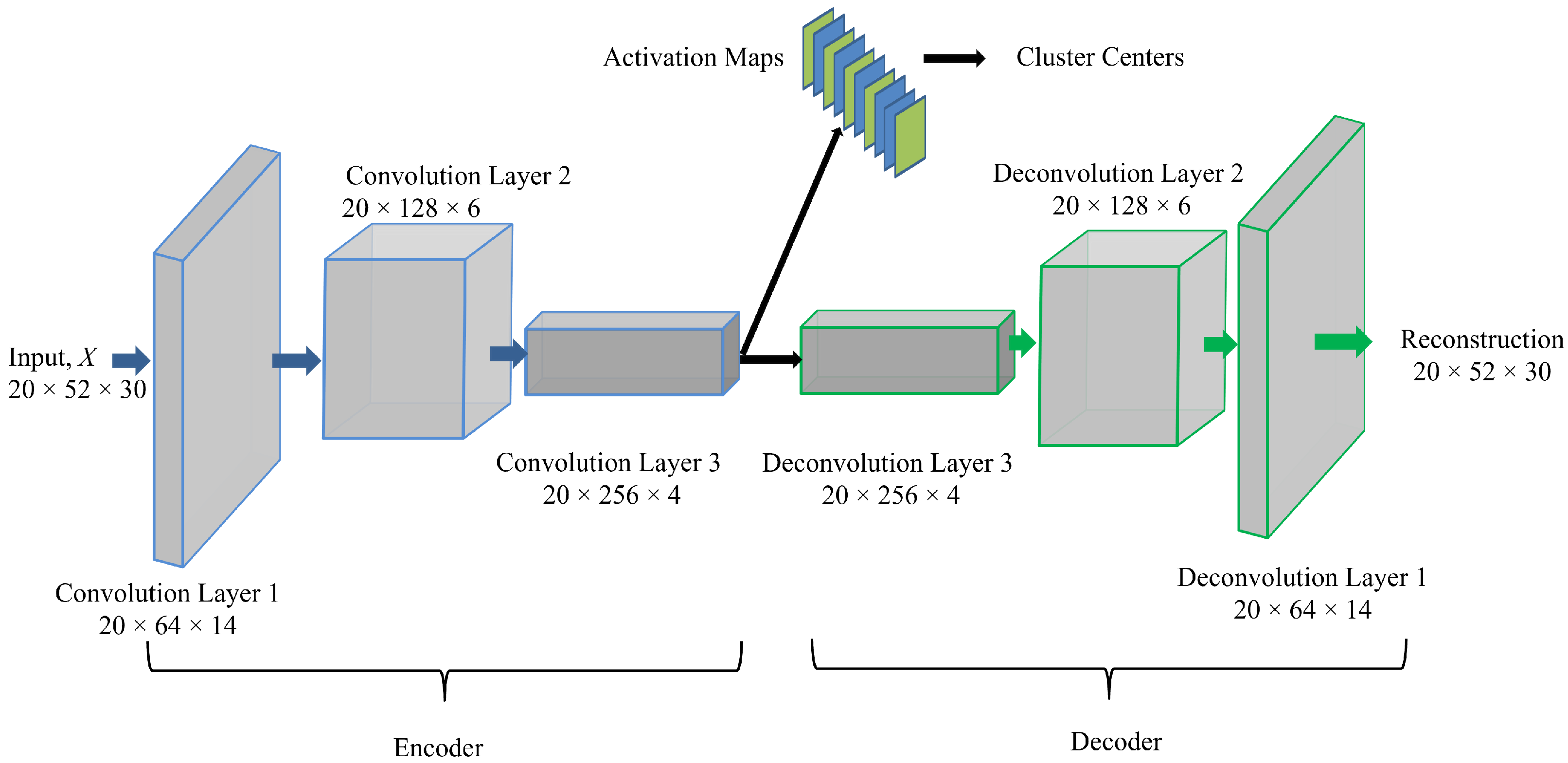
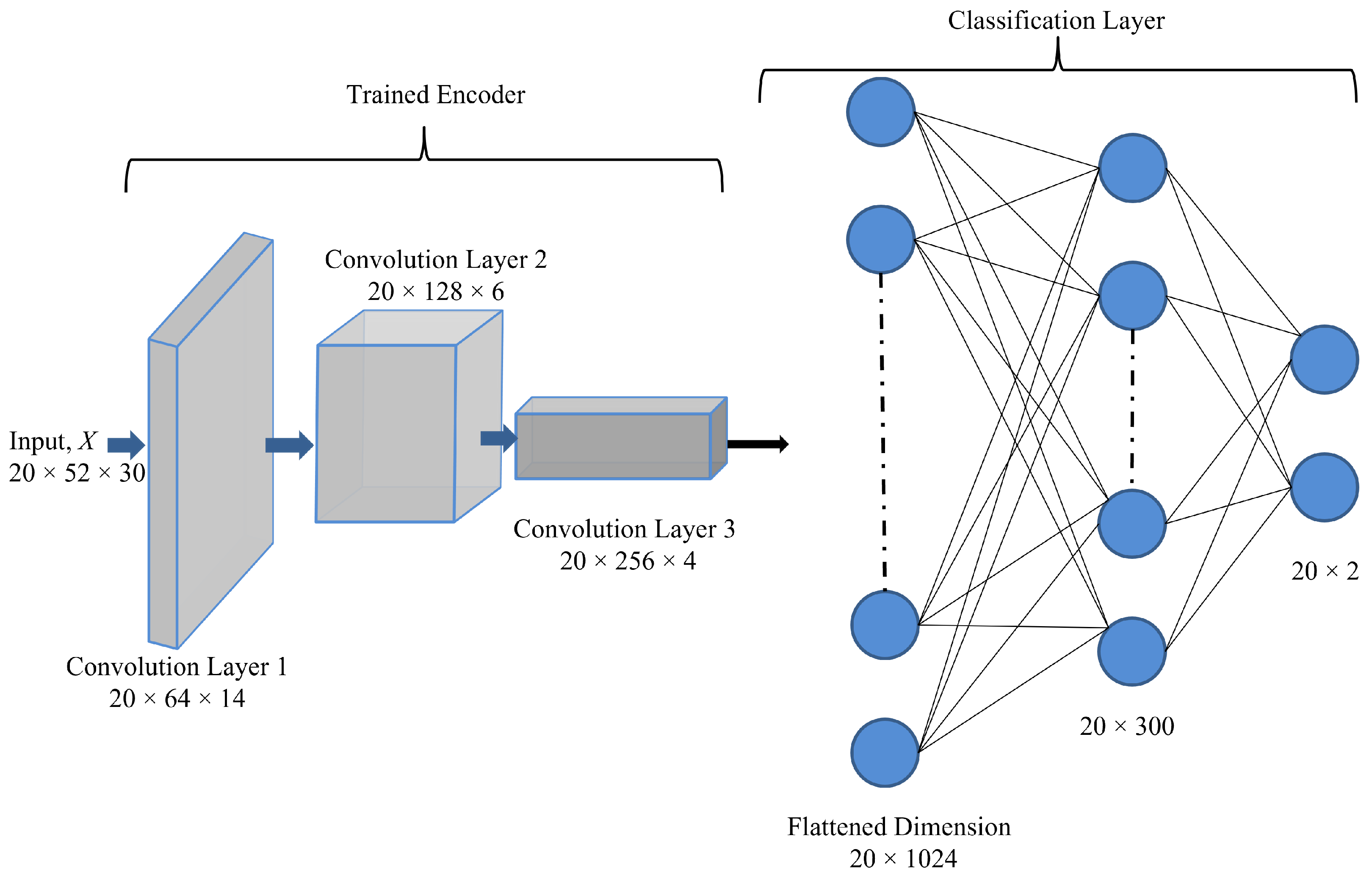
- Three convolution layers with the LeakyReLU [64] activation function
- A kernel size of 3 in all convolution layers
- The number of convolution channels doubling with each layer, starting with 64 channels.
- The number of clustering channels is set to 128 in the bottleneck layer.
- A batch-size of 20 with and is used.
- All the models are trained for 100 epochs with the stochastic gradient descent (SGD) optimizer with an penalty of 0.02.
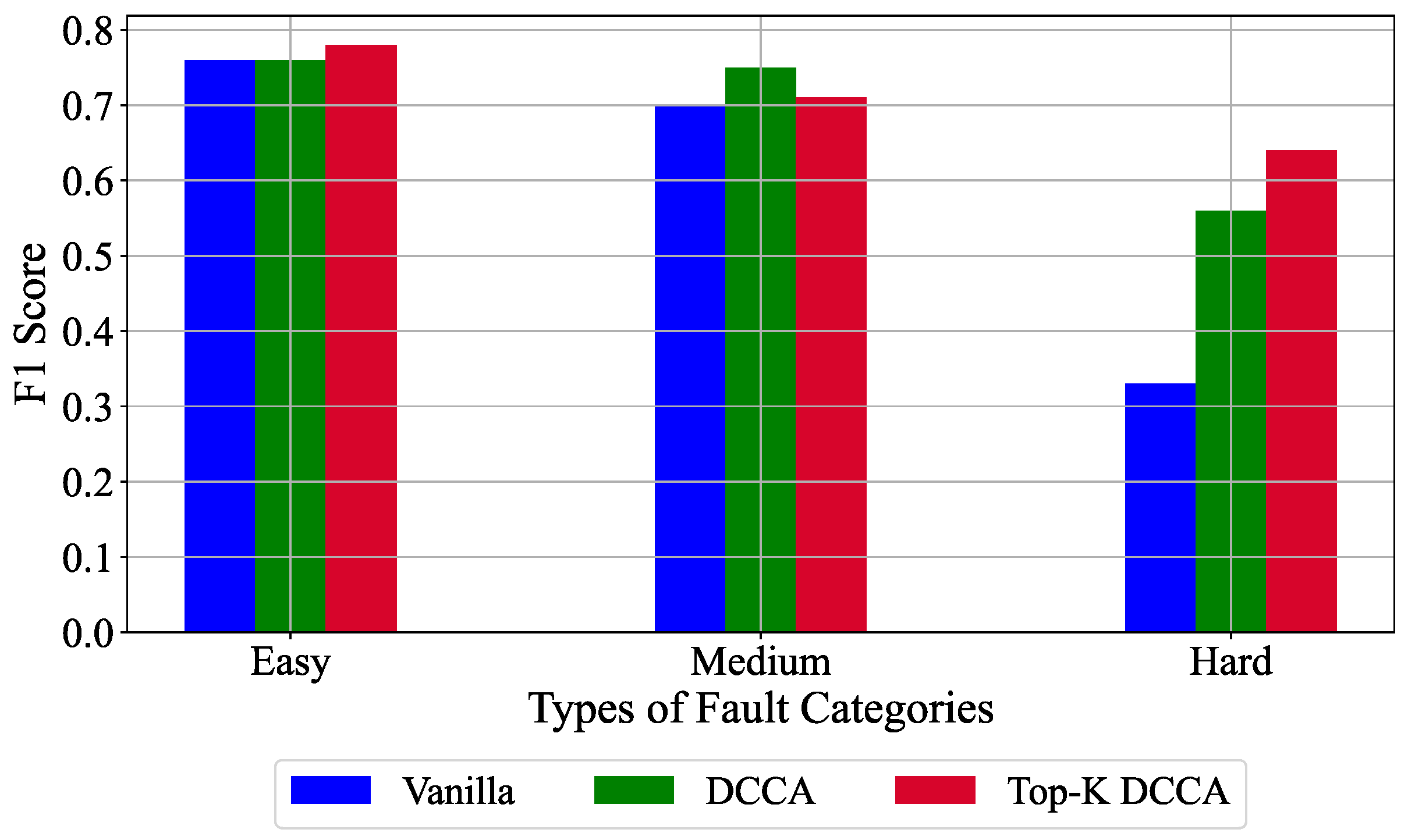
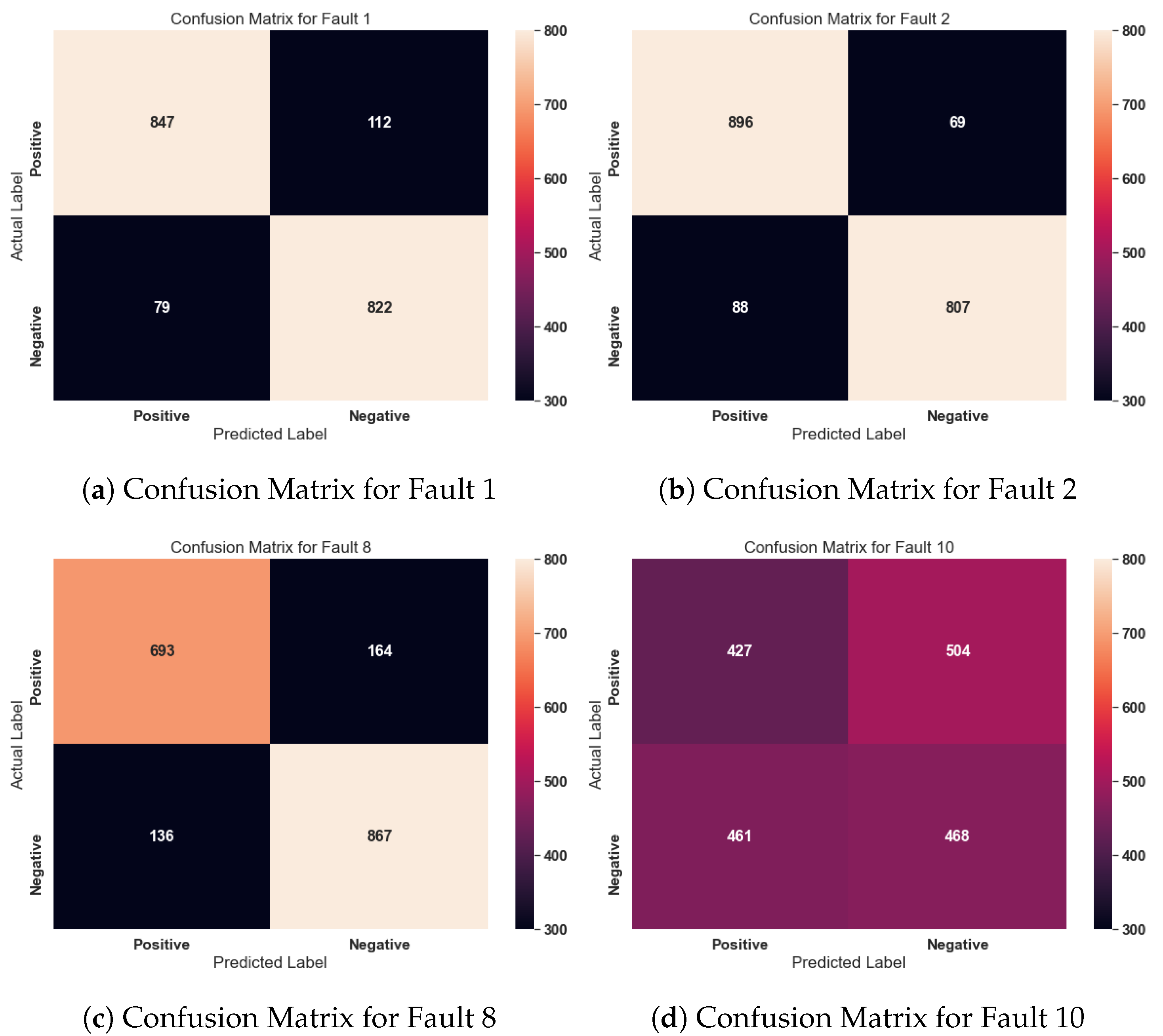
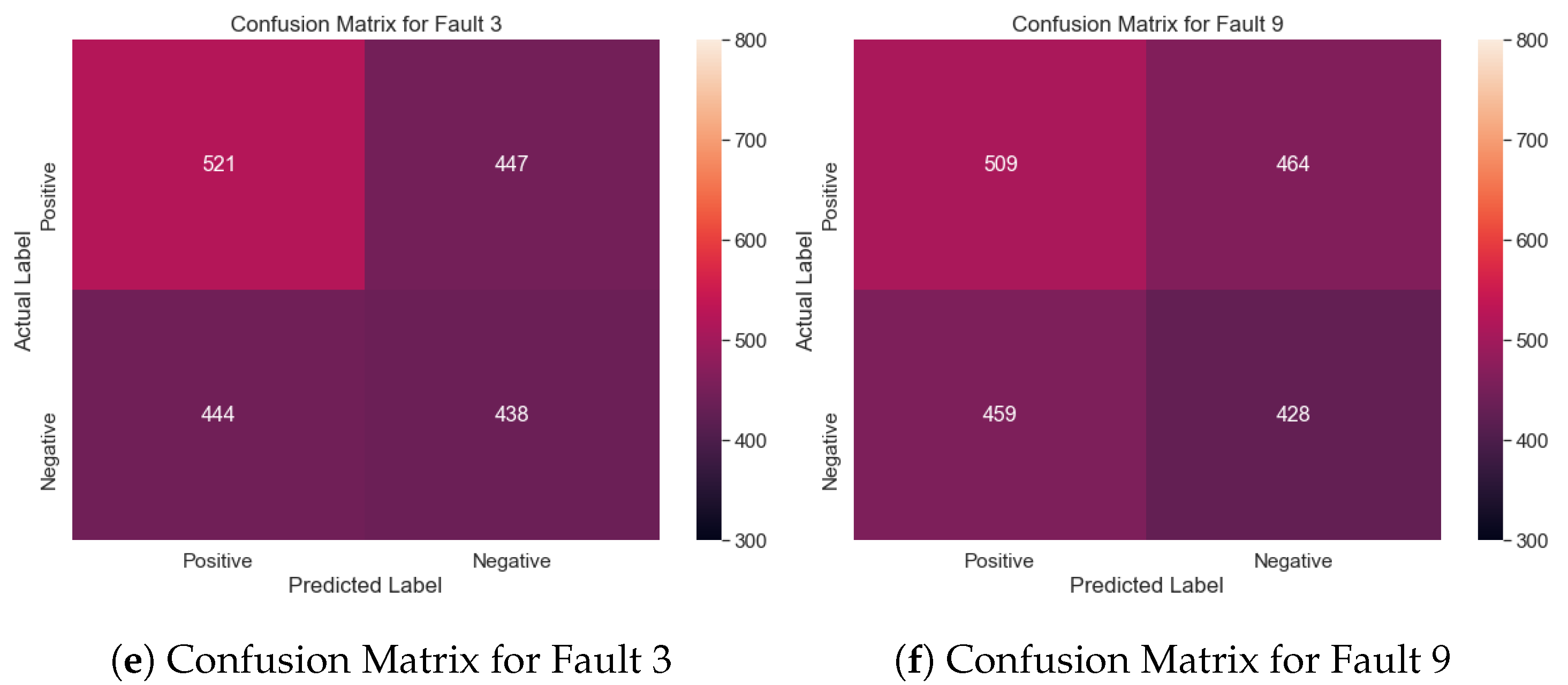
6.4. Semi-Supervised Learning Results
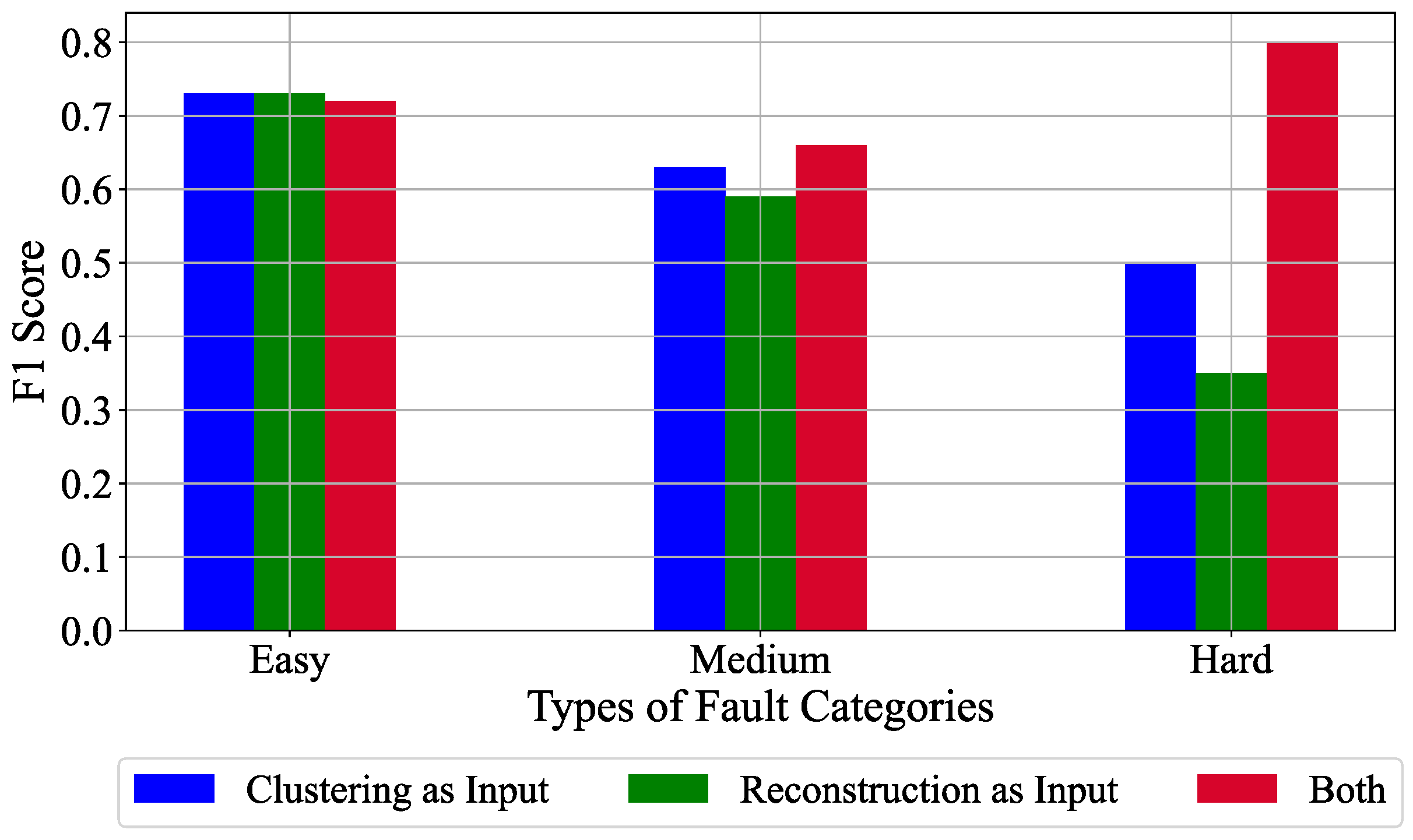
6.5. Classification Variants Results
6.6. Comparison with Literature
7. Conclusions
Author Contributions
Funding
Conflicts of Interest
Abbreviations
| DNN | Deep Neural Networks |
| CNN | Convolutional Neural Networks |
| AE | Autoencoder |
| CAE | Convolutional Autoencoder |
| VAE | Variational Autoencoder |
| GAN | Generative Adversarial Networks |
| TE | Tennessee Eastman |
| DCCA | Deep Convolutional Clustering Algorithm |
| LSTM | Long Short Term Memory |
References
- Chadha, G.S.; Panambilly, A.; Schwung, A.; Ding, S.X. Bidirectional deep recurrent neural networks for process fault classification. ISA Trans. 2020, 106, 330–342. [Google Scholar] [CrossRef] [PubMed]
- Da Xu, L.; He, W.; Li, S. Internet of things in industries: A survey. IEEE Trans. Ind. Inform. 2014, 10, 2233–2243. [Google Scholar]
- Pimentel, M.A.; Clifton, D.A.; Clifton, L.; Tarassenko, L. A review of novelty detection. Signal Process. 2014, 99, 215–249. [Google Scholar] [CrossRef]
- Ruff, L.; Kauffmann, J.R.; Vandermeulen, R.A.; Montavon, G.; Samek, W.; Kloft, M.; Dietterich, T.G.; Müller, K.-R. A Unifying Review of Deep and Shallow Anomaly Detection. Proc. IEEE 2021, 109, 756–795. [Google Scholar] [CrossRef]
- LeCun, Y.; Bengio, Y.; Hinton, G. Deep learning. Nature 2015, 521, 436–444. [Google Scholar] [CrossRef] [PubMed]
- Hinton, G.E. Connectionist learning procedures. Artif. Intell. 1989, 40, 185–234. [Google Scholar] [CrossRef] [Green Version]
- Goodfellow, I.; Pouget-Abadie, J.; Mirza, M.; Xu, B.; Warde-Farley, D.; Ozair, S.; Courville, A.; Bengio, Y. Generative Adversarial Nets. In Advances in Neural Information Processing Systems; Ghahramani, Z., Welling, M., Cortes, C., Lawrence, N., Weinberger, K.Q., Eds.; Curran Associates, Inc.: Red Hook, NY, USA, 2014; Volume 27, pp. 2672–2680. [Google Scholar]
- Vincent, P.; Larochelle, H.; Bengio, Y.; Manzagol, P.A. Extracting and composing robust features with denoising autoencoders. In Proceedings of the 25th International Conference on Machine Learning, Helsinki, Finland, 5–9 July 2008; pp. 1096–1103. [Google Scholar]
- Kingma, D.P.; Welling, M. An introduction to variational autoencoders. Found. Trends 2019, 12, 307–392. [Google Scholar]
- Makhzani, A.; Shlens, J.; Jaitly, N.; Goodfellow, I.; Frey, B. Adversarial autoencoders. arXiv 2015, arXiv:1511.05644. [Google Scholar]
- MacQueen, J. Some methods for classification and analysis of multivariate observations. In Proceedings of the Fifth Berkeley Symposium on Mathematical Statistics and Probability, Berkeley, CA, USA, 21 June–18 July 1965; Volume 1, pp. 281–297. [Google Scholar]
- Jain, A.K. Data clustering: 50 years beyond K-means. Pattern Recognit. Lett. 2010, 31, 651–666. [Google Scholar] [CrossRef]
- Downs, J.J.; Vogel, E.F. A plant-wide industrial process control problem. Comput. Chem. Eng. 1993, 17, 245–255. [Google Scholar] [CrossRef]
- Shiravi, A.; Shiravi, H.; Tavallaee, M.; Ghorbani, A.A. Toward developing a systematic approach to generate benchmark datasets for intrusion detection. Comput. Secur. 2012, 31, 357–374. [Google Scholar] [CrossRef]
- Ghosh, S.; Reilly, D.L. Credit card fraud detection with a neural-network. In Proceedings of the Twenty-Seventh Hawaii International Conference on System Sciences, Wailea, HI, USA, 4–7 January 1994; Volume 3, pp. 621–630. [Google Scholar] [CrossRef]
- Clifton, L.; Clifton, D.A.; Watkinson, P.J.; Tarassenko, L. Identification of patient deterioration in vital-sign data using one-class support vector machines. In Proceedings of the 2011 Federated Conference on Computer Science and Information Systems (FedCSIS), Szczecin, Poland, 18–21 September 2011; pp. 125–131. [Google Scholar]
- Venkatasubramanian, V.; Rengaswamy, R.; Kavuri, S.N.; Yin, K. A review of process fault detection and diagnosis: Part III: Process history based methods. Comput. Chem. Eng. 2003, 27, 327–346. [Google Scholar] [CrossRef]
- Yin, S.; Ding, S.X.; Xie, X.; Luo, H. A review on basic data-driven approaches for industrial process monitoring. IEEE Trans. Ind. Electron. 2014, 61, 6418–6428. [Google Scholar] [CrossRef]
- Gao, Z.; Cecati, C.; Ding, S.X. A Survey of Fault Diagnosis and Fault-Tolerant Techniques—Part II: Fault Diagnosis with Knowledge-Based and Hybrid/Active Approaches. IEEE Trans. Ind. Electron. 2015, 62, 3768–3774. [Google Scholar] [CrossRef] [Green Version]
- Giantomassi, A.; Ferracuti, F.; Iarlori, S.; Ippoliti, G.; Longhi, S. Electric Motor Fault Detection and Diagnosis by Kernel Density Estimation and Kullback–Leibler Divergence Based on Stator Current Measurements. IEEE Trans. Ind. Electron. 2015, 62, 1770–1780. [Google Scholar] [CrossRef]
- Yin, S.; Ding, S.X.; Haghani, A.; Hao, H.; Zhang, P. A comparison study of basic data-driven fault diagnosis and process monitoring methods on the benchmark Tennessee Eastman process. J. Process. Control. 2012, 22, 1567–1581. [Google Scholar] [CrossRef]
- He, Q.P.; Wang, J. Fault detection using the k-nearest neighbor rule for semiconductor manufacturing processes. IEEE Trans. Semicond. Manuf. 2007, 20, 345–354. [Google Scholar] [CrossRef]
- Mahadevan, S.; Shah, S.L. Fault detection and diagnosis in process data using one-class support vector machines. J. Process. Control. 2009, 19, 1627–1639. [Google Scholar] [CrossRef]
- Khan, S.; Yairi, T. A review on the application of deep learning in system health management. Mech. Syst. Signal Process. 2018, 107, 241–265. [Google Scholar] [CrossRef]
- Zhao, R.; Yan, R.; Chen, Z.; Mao, K.; Wang, P.; Gao, R.X. Deep learning and its applications to machine health monitoring. Mech. Syst. Signal Process. 2019, 115, 213–237. [Google Scholar] [CrossRef]
- Zhang, L.; Lin, J.; Liu, B.; Zhang, Z.; Yan, X.; Wei, M. A Review on Deep Learning Applications in Prognostics and Health Management. IEEE Access 2019, 7, 162415–162438. [Google Scholar] [CrossRef]
- Lei, Y.; Yang, B.; Jiang, X.; Jia, F.; Li, N.; Nandi, A.K. Applications of machine learning to machine fault diagnosis: A review and roadmap. Mech. Syst. Signal Process. 2020, 138, 106587. [Google Scholar] [CrossRef]
- Chalapathy, R.; Chawla, S. Deep learning for anomaly detection: A survey. arXiv 2019, arXiv:1901.03407. [Google Scholar]
- Schlegl, T.; Seeböck, P.; Waldstein, S.M.; Schmidt-Erfurth, U.; Langs, G. Unsupervised Anomaly Detection with Generative Adversarial Networks to Guide Marker Discovery. In Information Processing in Medical Imaging; Niethammer, M., Ed.; Springer: Cham, Switzerland, 2017; Volume 10265, pp. 146–157. [Google Scholar] [CrossRef] [Green Version]
- Akcay, S.; Atapour-Abarghouei, A.; Breckon, T.P. GANomaly: Semi-supervised Anomaly Detection via Adversarial Training. In Computer Vision—ACCV 2018; Jawahar, C.V., Li, H., Mori, G., Schindler, K., Eds.; Springer: Cham, Switzerland, 2019; Volume 11363, pp. 622–637. [Google Scholar] [CrossRef] [Green Version]
- Liu, H.; Zhou, J.; Xu, Y.; Zheng, Y.; Peng, X.; Jiang, W. Unsupervised fault diagnosis of rolling bearings using a deep neural network based on generative adversarial networks. Neurocomputing 2018, 315, 412–424. [Google Scholar] [CrossRef]
- Wang, Z.; Wang, J.; Wang, Y. An intelligent diagnosis scheme based on generative adversarial learning deep neural networks and its application to planetary gearbox fault pattern recognition. Neurocomputing 2018, 310, 213–222. [Google Scholar] [CrossRef]
- Arjovsky, M.; Bottou, L. Towards principled methods for training generative adversarial networks. arXiv 2017, arXiv:1701.04862. [Google Scholar]
- Hinton, G.E.; Salakhutdinov, R.R. Reducing the dimensionality of data with neural networks. Science 2006, 313, 504–507. [Google Scholar] [CrossRef] [Green Version]
- Pawlowski, N.; Lee, M.C.H.; Rajchl, M.; McDonagh, S.; Ferrante, E.; Kamnitsas, K.; Cooke, S.; Stevenson, S.; Khetani, A.; Newman, T.; et al. Unsupervised lesion detection in brain CT using bayesian convolutional autoencoders. In Proceedings of the International Conference on Medical Imaging with Deep Learning (MIDL), Amsterdam, The Netherlands, 4–6 July 2018. [Google Scholar]
- Yang, H.; Wang, B.; Lin, S.; Wipf, D.; Guo, M.; Guo, B. Unsupervised extraction of video highlights via robust recurrent auto-encoders. In Proceedings of the IEEE International Conference on Computer Vision, Santiago, Chile, 7–13 December 2015; pp. 4633–4641. [Google Scholar]
- Zong, B.; Song, Q.; Min, M.R.; Cheng, W.; Lumezanu, C.; Cho, D.; Chen, H. Deep autoencoding gaussian mixture model for unsupervised anomaly detection. In Proceedings of the International Conference on Learning Representations, Vancouver, BC, Canada, 30 April–3 May 2018. [Google Scholar]
- Hu, B.; Gao, B.; Woo, W.L.; Ruan, L.; Jin, J.; Yang, Y.; Yu, Y. A Lightweight Spatial and Temporal Multi-Feature Fusion Network for Defect Detection. IEEE Trans. Image Process. 2021, 30, 472–486. [Google Scholar] [CrossRef]
- Ahmed, J.; Gao, B.; Woo, W.L. Sparse Low-Rank Tensor Decomposition for Metal Defect Detection Using Thermographic Imaging Diagnostics. IEEE Trans. Ind. Inform. 2021, 17, 1810–1820. [Google Scholar] [CrossRef]
- Wang, Y.; Yang, H.; Yuan, X.; Shardt, Y.A.; Yang, C.; Gui, W. Deep learning for fault-relevant feature extraction and fault classification with stacked supervised auto-encoder. J. Process. Control 2020, 92, 79–89. [Google Scholar] [CrossRef]
- Gong, D.; Liu, L.; Le, V.; Saha, B.; Mansour, M.R.; Venkatesh, S.; van den Hengel, A. Memorizing Normality to Detect Anomaly: Memory-Augmented Deep Autoencoder for Unsupervised Anomaly Detection. In Proceedings of the 2019 IEEE/CVF International Conference on Computer Vision (ICCV), Seoul, Korea, 27 Decemder–2 November 2019; pp. 1705–1714. [Google Scholar] [CrossRef] [Green Version]
- Ruff, L.; Vandermeulen, R.; Goernitz, N.; Deecke, L.; Siddiqui, S.A.; Binder, A.; Müller, E.; Kloft, M. Deep one-class classification. In Proceedings of the 35th International Conference on Machine Learning, Stockholm, Sweden, 10–15 July 2018; pp. 4393–4402. [Google Scholar]
- Qi, Y.; Shen, C.; Wang, D.; Shi, J.; Jiang, X.; Zhu, Z. Stacked Sparse Autoencoder-Based Deep Network for Fault Diagnosis of Rotating Machinery. IEEE Access 2017, 5, 15066–15079. [Google Scholar] [CrossRef]
- Sun, W.; Shao, S.; Zhao, R.; Yan, R.; Zhang, X.; Chen, X. A sparse auto-encoder-based deep neural network approach for induction motor faults classification. Measurement 2016, 89, 171–178. [Google Scholar] [CrossRef]
- Wang, L.; Zhang, Z.; Xu, J.; Liu, R. Wind Turbine Blade Breakage Monitoring with Deep Autoencoders. IEEE Trans. Smart Grid 2018, 9, 2824–2833. [Google Scholar] [CrossRef]
- Jiang, G.; Xie, P.; He, H.; Yan, J. Wind Turbine Fault Detection Using a Denoising Autoencoder With Temporal Information. IEEE/ASME Trans. Mechatron. 2018, 23, 89–100. [Google Scholar] [CrossRef]
- Liu, C.; Ghosal, S.; Jiang, Z.; Sarkar, S. An Unsupervised Spatiotemporal Graphical Modeling Approach to Anomaly Detection in Distributed CPS. In Proceedings of the 7th International Conference on Cyber-Physical Systems, Vienna, Austria, 11–14 April 2016. [Google Scholar]
- Yan, W.; Guo, P.; Gong, L.; Li, Z. Nonlinear and robust statistical process monitoring based on variant autoencoders. Chemom. Intell. Lab. Syst. 2016, 158, 31–40. [Google Scholar] [CrossRef]
- Chadha, G.S.; Rabbani, A.; Schwung, A. Comparison of Semi-supervised Deep Neural Networks for Anomaly Detection in Industrial Processes. In Proceedings of the 2019 IEEE 17th International Conference on Industrial Informatics (INDIN), Helsinki-Espoo, Finland, 22–25 July 2019; Volume 1, pp. 214–219. [Google Scholar] [CrossRef]
- Kim, C.; Lee, J.; Kim, R.; Park, Y.; Kang, J. DeepNAP: Deep neural anomaly pre-detection in a semiconductor fab. Inf. Sci. 2018, 457–458, 1–11. [Google Scholar] [CrossRef]
- Masci, J.; Meier, U.; Cireşan, D.; Schmidhuber, J. Stacked convolutional auto-encoders for hierarchical feature extraction. In International Conference on Artificial Neural Networks; Springer: Berlin/Heidelberg, Germany, 2011; pp. 52–59. [Google Scholar]
- Tran, H.T.M.; Hogg, D. Anomaly detection using a convolutional winner-take-all autoencoder. In Proceedings of the British Machine Vision Conference 2017, London, UK, 4–7 September 2017. [Google Scholar]
- Ribeiro, M.; Lazzaretti, A.E.; Lopes, H.S. A study of deep convolutional auto-encoders for anomaly detection in videos. Pattern Recognit. Lett. 2018, 105, 13–22. [Google Scholar] [CrossRef]
- Zhang, C.; Song, D.; Chen, Y.; Feng, X.; Lumezanu, C.; Cheng, W.; Ni, J.; Zong, B.; Chen, H.; Chawla, N.V. A deep neural network for unsupervised anomaly detection and diagnosis in multivariate time series data. In Proceedings of the AAAI Conference on Artificial Intelligence, Honolulu, HI, USA, 27 January–1 February 2019; Volume 33, pp. 1409–1416. [Google Scholar]
- Yang, B.; Fu, X.; Sidiropoulos, N.D.; Hong, M. Towards k-means-friendly spaces: Simultaneous deep learning and clustering. In Proceedings of the 34th International Conference on Machine Learning, Sydney, Australia, 6–11 August 2017; Volume 70, pp. 3861–3870. [Google Scholar]
- Guo, X.; Liu, X.; Zhu, E.; Yin, J. Deep clustering with convolutional autoencoders. In International Conference on Neural Information Processing; Springer: Cham, Switzerland, 2017; pp. 373–382. [Google Scholar]
- Caron, M.; Bojanowski, P.; Joulin, A.; Douze, M. Deep Clustering for Unsupervised Learning of Visual Features. In Proceedings of the European Conference on Computer Vision (ECCV), Munich, Germany, 8–14 September 2018. [Google Scholar]
- Ghasedi Dizaji, K.; Herandi, A.; Deng, C.; Cai, W.; Huang, H. Deep Clustering via Joint Convolutional Autoencoder Embedding and Relative Entropy Minimization. In Proceedings of the IEEE International Conference on Computer Vision (ICCV), Venice, Italy, 22–29 October 2017. [Google Scholar]
- Banerjee, A.; Merugu, S.; Dhillon, I.S.; Ghosh, J. Clustering with Bregman divergences. J. Mach. Learn. Res. 2005, 6, 1705–1749. [Google Scholar]
- Xu, W.; Liu, X.; Gong, Y. Document Clustering Based on Non-Negative Matrix Factorization. In Proceedings of the 26th Annual International ACM SIGIR Conference on Research and Development in Informaion Retrieval, Toronto, ON, Canada, 28 July–1 August 2003; Association for Computing Machinery: New York, NY, USA, 2003; pp. 267–273. [Google Scholar] [CrossRef]
- Bruna, J.; Mallat, S. Invariant Scattering Convolution Networks. IEEE Trans. Pattern Anal. Mach. Intell. 2013, 35, 1872–1886. [Google Scholar] [CrossRef] [Green Version]
- Chadha, G.S.; Panara, U.; Schwung, A.; Ding, S.X. Generalized dilation convolutional neural networks for remaining useful lifetime estimation. Neurocomputing 2021, 452, 182–199. [Google Scholar] [CrossRef]
- Rumelhart, D.E.; Hinton, G.E.; Williams, R.J. Learning representations by back-propagating errors. Nature 1986, 323, 533–536. [Google Scholar] [CrossRef]
- Maas, A.L.; Hannun, A.Y.; Ng, A.Y. Rectifier nonlinearities improve neural network acoustic models. In Proceedings of the International Conference on Machine Learning, Atlanta, GA, USA, 16–21 June 2013; Volume 30, p. 3. [Google Scholar]
- Van der Maaten, L.; Hinton, G. Visualizing Data using t-SNE. J. Mach. Learn. Res. 2008, 9, 2579–2605. [Google Scholar]
- Rato, T.J.; Reis, M.S. Fault detection in the Tennessee Eastman benchmark process using dynamic principal components analysis based on decorrelated residuals (DPCA-DR). Chemom. Intell. Lab. Syst. 2013, 125, 101–108. [Google Scholar] [CrossRef]
- Russell, E.L.; Chiang, L.H.; Braatz, R.D. Fault detection in industrial processes using canonical variate analysis and dynamic principal component analysis. Chemom. Intell. Lab. Syst. 2000, 51, 81–93. [Google Scholar] [CrossRef]
- Bagnall, A.; Lines, J.; Bostrom, A.; Large, J.; Keogh, E. The great time series classification bake off: A review and experimental evaluation of recent algorithmic advances. Data Min. Knowl. Discov. 2017, 31, 606–660. [Google Scholar] [CrossRef] [PubMed] [Green Version]


| Fault Cases | Description | Type |
|---|---|---|
| 1 | A/C ratio, B composition constant (Stream 4) | Step |
| 2 | B composition, A/C ratio constant (Stream 4) | Step |
| 3 | D feed temperature (Stream 2) | Step |
| 4 | Reactor cooling water supply temperature | Step |
| 5 | Condenser cooling water supply temperature | Step |
| 6 | A feed loss (Stream 1) | Step |
| 7 | C header pressure loss (Stream 4) | Step |
| 8 | A, B, C feed composition (Stream 4) | Random |
| 9 | D feed temperature (Stream 2) | Random |
| 10 | C feed temperature (Stream 4) | Random |
| 11 | Reactor cooling water supply temperature | Random |
| 12 | Condenser cooling water supply temperature | Random |
| 13 | Reaction Kinetics | Slow drift |
| 14 | Reactor cooling water valve | Sticking |
| 15 | Condenser cooling water valve | Sticking |
| 16 | Unknown | - |
| 17 | Unknown | - |
| 18 | Unknown | - |
| 19 | Unknown | - |
| 20 | Unknown | - |
| 21 | A, B, C feed valve (Stream 4) | Constant position |
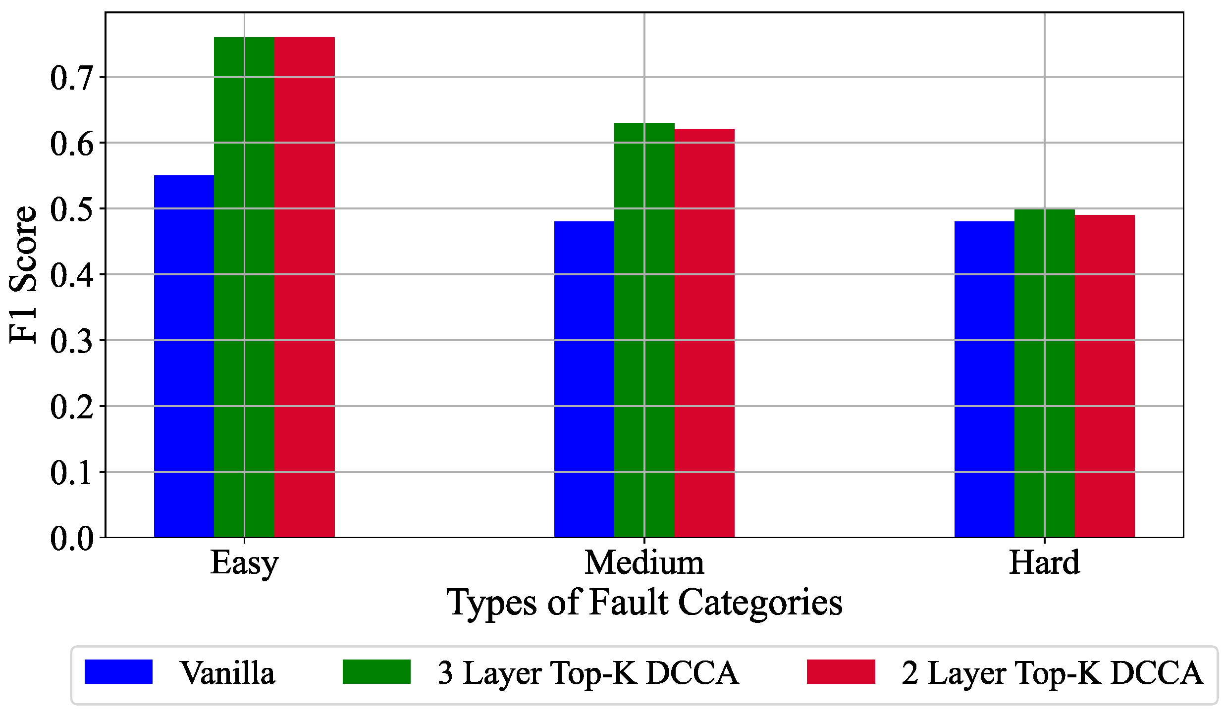
| Subgroup | Normal Case | Fault Cases |
|---|---|---|
| Easy | 0 | 1, 2, 4, 5, 6, 7, 12, 14, 18 |
| Medium | 0 | 8, 10, 11, 13, 16, 17, 19, 20 |
| Hard | 0 | 3, 9, 15, 21 |
| Fault Case | Top-K DCCA | [21] | [66] | [67] | DAE [49] | Denoising DAE [49] |
|---|---|---|---|---|---|---|
| (3) | 53.82 | 4.5 | 2.1 | 1.4 | 16.66 | 16.67 |
| (9) | 52.31 | 4.75 | 2 | 0.7 | 16.87 | 16.97 |
| (15) | 43.98 | 7.75 | 38.5 | 9.7 | 17.08 | 17.08 |
| (21) | 50.05 | 56.38 | 53.9 | 65.8 | 44.37 | 45 |
| Overall | 50.04 | 18.34 | 24.12 | 19.4 | 23.74 | 23.93 |
Publisher’s Note: MDPI stays neutral with regard to jurisdictional claims in published maps and institutional affiliations. |
© 2021 by the authors. Licensee MDPI, Basel, Switzerland. This article is an open access article distributed under the terms and conditions of the Creative Commons Attribution (CC BY) license (https://creativecommons.org/licenses/by/4.0/).
Share and Cite
Chadha, G.S.; Islam, I.; Schwung, A.; Ding, S.X. Deep Convolutional Clustering-Based Time Series Anomaly Detection. Sensors 2021, 21, 5488. https://doi.org/10.3390/s21165488
Chadha GS, Islam I, Schwung A, Ding SX. Deep Convolutional Clustering-Based Time Series Anomaly Detection. Sensors. 2021; 21(16):5488. https://doi.org/10.3390/s21165488
Chicago/Turabian StyleChadha, Gavneet Singh, Intekhab Islam, Andreas Schwung, and Steven X. Ding. 2021. "Deep Convolutional Clustering-Based Time Series Anomaly Detection" Sensors 21, no. 16: 5488. https://doi.org/10.3390/s21165488