Passive Measurement of Three Optical Beacon Coordinates Using a Simultaneous Method

Abstract

Among other things, passive methods based on the processing of images of feature points or beacons captured by an image sensor are used to measure the relative position of objects. At least two cameras usually have to be used to obtain the required information, or the cameras are combined with other sensors working on different physical principles. This paper describes the principle of passively measuring three position coordinates of an optical beacon using a simultaneous method and presents the results of corresponding experimental tests. The beacon is represented by an artificial geometric structure, consisting of several semiconductor light sources. The sources are suitably arranged to allow, all from one camera, passive measurement of the distance, two position angles, the azimuth, and the beacon elevation. The mathematical model of this method consists of working equations containing measured coordinates, geometric parameters of the beacon, and geometric parameters of the beacon image captured by the camera. All the results of these experimental tests are presented.

1. Introduction

The article describes how to measure a position of an artificially created object, an optical beacon (hereinafter beacon), in relation to one measuring camera (hereinafter camera). The below presented simultaneous analytical method is one of the passive methods for measuring an object’s relative position.

1.1. Problem Statement

The measurement of object position is an important problem that is solved in numerous areas of human activities. Many different instruments and methods have been developed for outdoor and indoor positioning.

Passive methods using images of some objects of interest constitute one group of methods of measuring the relative position of objects. Some analytical methods are theoretically developed, experimentally verified, and practically used as well [1,2,3,4,5,6]. There are some studies that use stereo vision for measuring position [7,8] or a combination of one camera and another sensor such as a sonar or laser range finder [9,10]. Cameras are also used along with inertial navigation systems [7,11]. This task can be solved using neural networks as well [12,13].

The proposed passive method does not require complex and extensive instrumentation. It needs one camera as the only sensor. On the other hand, the necessary condition for the application of this method is the use of a specific system of feature points, which have to be defined on a surface of the object of interest. The feature points do not have to transmit a specific optical signal. They can create an artificial beacon, which serves as a reference object for a measuring unit equipped with an image sensor. The paper presents a positioning system of this type. Due to the design of the beacon, spans of measured angular coordinates are constrained. However, the beacon layout can be modified so that a span of measured values of position angles is significantly extended.

1.2. Literature Review

A number of different techniques have been developed for indoor positioning systems. Some of these methods are based on evaluating either the time of arrival (TOA) or the time difference of arrival (TDOA) of an optical signal to the receiver; others are based on the received signal strength (RSS) depending on the receiver position [14,15,16,17], and there are also methods based on a receiver position determination according to the angle of arrival (AOA) [18,19,20,21,22,23,24]. Time methods use modulated signal travel time between several reference sources and a receiver. If the source irradiance spatial pattern is known, e.g., light-emitting diode (LED) [25], certain angle methods use the dependence of the received signal strength on the incident angle and on the angle between the normal radiation source and the direction to the receiver. Position angles can be determined also without knowledge of the radiation spatial distribution [16]. Other methods utilize the dependence of a position or of individual source image sizes in the plane of the image sensor [22,26]. The AOA method is also used in a quadrant angular diversity aperture (QADA) receiver, which is equipped with a quadrant photodiode (PD) and an aperture shifted from the PD plane by a small distance. The QADA receiver can be combined with an image sensor [27].

Measuring systems consist of one or several radiation sources and receivers. The radiation of the fixed reference sources located in a room, for example on the ceiling, can be modulated in accordance with the applied method. The sources’ coordinates have to be known. The predominant, but not the only, radiation source type is LED semiconductor. Photodiodes [14,16] or image sensors [18,19,20,21] or both together are used to detect radiation on the receiver side. Optoelectronic receivers can be combined with magnetic field sensors [23], accelerometers [14,16], gyroscopes, or inertial navigation systems, depending on the method [24]. Active optoelectronic sensors, e.g., lidars, are utilized too [22]. Utilization of the scale-invariant feature transform (SIFT) method is described in [18]. Indoor positioning systems also use artificial neural networks (see [18,24,28,29]). Feature points can have an arbitrary nature. In order to be identifiable, they need to be sufficiently contrasting. No specific radiation pattern needs to be assumed to determine the beacon position. The measuring error of the position coordinates is in the order of centimeters when the radiation sources and the receivers are at a distance in the order of meters.

1.3. Principle of the Simultaneous Analytical Method

The solution presented in this article is based on the utilization of one camera. We use the specific object, beacon, and the simultaneous measurement of individual quantities. This method provides the possibility of measuring three positional coordinates if the transverse axis of the beacon and the transverse axis of the camera lie in parallel planes. The diagram of the beacon made for experimental test purposes is shown in Figure 1 [30,31], where A_f is the beacon front wall; A_slp and A_srp are projections of the left and right beacon side walls, respectively; b, d₁₆, α₁, and β are parameters of the beacon; C_B is the center of the beacon; S₁ to S₉ are light sources (S₁ is the reference light source); S₁x_By_Bz_B is the beacon coordinate system; and ρ_h and ρ_v are the horizontal and vertical planes, respectively.

The beacon enables satisfactory measurement of the distance between the beacon and the camera R (hereinafter beacon distance), the beacon position angle in a horizontal plane ω (hereinafter azimuth), and the beacon elevation angle ψ (hereinafter elevation). The angles are created by rotating the beacon around its transverse axes z_ρωψ0 and y_B, respectively (see Figure 2), where Cx_Cy_Cz_C is the camera coordinate system, S₁x_ωy_ρωψ0z_ρωψ0 is the reference coordinate system, and γ_r is a mutual tilt between the camera and the beacon. Nine semiconductor light sources of LED type (hereinafter diodes) represent sources of the optical signals, which are captured by the camera. According to the mutual position of the diodes on the beacon, and according to the diodes’ mutual position in their images in the plane of the camera sensor, the desired quantities can be then determined. The diodes create three square walls of the beacon with side b: a front wall A_f and two side walls, left A_sl and right A_sr. The main parameters of the beacon are the base b and the beacon opening angle β. The side wall projection sizes A_slp and A_srp depend on these parameters.

The evaluation of the position of the beacon diode images was done manually. The position coordinates were calculated and the measurement results were processed on a personal computer. Nowadays, the practical use of this method in real time is not possible. To do this, it is necessary to make a purpose-built automatic measuring device and to create the necessary software similar to those described in [32], where a smaller version of the optical beacon is used. A basic unsolved task is the measurement of the real range of the system for which the position coordinates reach their limits determined by the permissible errors.

The aim of the paper is to explain the method principle and to present the test results obtained during the experiments verifying the suitability of the simultaneous analytical method for measuring the beacon distance, azimuth, and elevation. The rest of the paper is organized as follows: The simultaneous analytical method is described in Section 2. Section 3 provides experimental test results. Sources of errors are characterized in Section 4. Section 5 details ways of mathematical model adjustment. Section 6 presents the conclusion.

2. Description of the Simultaneous Analytical Method

The simultaneous analytical method for measuring two position coordinates was published in [30,31]. In these publications, we use working equations enabling measurement of the beacon distance R and the azimuth ω. These equations represent a mathematical model of this method. The method principle consists in a calculation of several so-called functional beacon distances (hereinafter functional distances) based on known distances between the two selected diodes and the measured distances between images of these diodes that were captured by the camera. Measuring two coordinates, as presented in [30,31], enables the determination of the position of an object only in the 2D plane. The only position coordinate on which the working equations depend is the azimuth ω. Functional distances were calculated for the so-called functional diodes S₂, S₃, S₆, and S₈ according to projections onto the y_ρψω0 axis. The problem can be solved only with the use of the functional distances for the diodes S₆ and S₈. When measuring the beacon position in the plane, the functional distance equation for the diode S₈, for example, is as follows [30,31]:

$$R_{81}=f\cdot \left[\frac{d_{16}\cdot \cos \left({\mathsf{\alpha }}_1-\mathsf{\omega }\right)}{b_{81}^{\prime }}-1\right]-d_{16}\cdot \sin \left({\mathsf{\alpha }}_1-\mathsf{\omega }\right),$$

(1)

where b^’₈₁ is the distance between the image of the S₁ reference diode and the image of the S₈ functional diode in the plane of the camera detector and d₁₆ and α₁ are the parameters of the beacon (see Figure 1).

For the measurement of the position of an object in 3D, the mathematical model had to be extended by at least one functional distance of one of the functional diodes S₄, S₅, S₇, and S₉, which lie on the lower line of the beacon. The working equations had to be adjusted also to include projections onto the z_ρψω0 axis, if they exist, which depend on both azimuth ω and elevation ψ. At least three functional distances have to be used as working equations. Such equations have to be chosen that their manifestation for at least one pair of functional diodes is opposite for both position angles. The chosen calculation uses parallel projections of the distances, between the reference diode S₁ and all eight functional diodes S₂ to S_9, onto appropriate axes of the reference rectangular coordinate system. Its axis xω is identical to the optical axis of the camera x_C. Then, for one particular functional diode, its functional distance for the provided azimuth and elevation is the calculated distance between the reference diode and the camera. The working equations are derived from the lens equations of the projections of the distances between the relevant diodes.

The angles ω and ψ are unknown variables that are computed as the numbers for which the deviation between the beacon functional distances, for the individual functional diodes, is a minimum. In other words, we are looking for the minimum of the root mean square (rms) of the difference D_rms between the individual functional distances and the mean of these functional distances. When the minimum is reached, the set azimuth, the set elevation, and the mean of the calculated functional distances are equal to the desired measured variables ω_m, ψ_m, and R_m, respectively. The following formulas, i.e., the working equations for the functional diodes S₃, S₅, S₈, and S₉ represent the mathematical model of this method:

$$R_{31}=f\cdot \left(\frac{P{S}_{3\mathsf{\rho }\mathsf{\omega }\mathsf{\psi }0}^{}}{b_{31y}^{}}-1\right)-P{S}_{3x\mathsf{\omega }}^{},$$

(2)

where $P{S}_{3x\mathsf{\omega }}^{}=-0.5\cdot b\cdot \sin \mathsf{\omega }$ and $P{S}_{3\mathsf{\rho }\mathsf{\omega }\mathsf{\psi }0}^{}=0.5\cdot b\cdot \cos \left(-\mathsf{\omega }\right)$;

$$R_{51}=f\cdot \left[\frac{\sqrt{{\left(P{S}_{5\mathsf{\rho }\mathsf{\omega }\mathsf{\psi }0}^y\right)}^2+{\left(P{S}_{5\mathsf{\rho }\mathsf{\omega }\mathsf{\psi }0}^z\right)}^2}}{\sqrt{b_{51y}^2+b_{51z}^2}}-1\right]-P{S}_{5x\mathsf{\omega }}^{},$$

(3)

where $P{S}_{5x\mathsf{\omega }}^{}=-0.5\cdot b\cdot \sin {\mathsf{\omega }+\mathsf{\delta }}_{x\mathsf{\psi }5}$, $P{S}_{5\mathsf{\rho }\mathsf{\omega }\mathsf{\psi }0}^y=0.5\cdot b\cdot \cos {\mathsf{\omega }+\mathsf{\delta }}_{y\mathsf{\psi }5}$, $P{S}_{5\mathsf{\rho }\mathsf{\omega }\mathsf{\psi }0}^z=b\cdot \cos \mathsf{\psi }$, ${\mathsf{\delta }}_{x\mathsf{\psi }5}=b\cdot \sin \mathsf{\psi }\cdot \cos \mathsf{\omega }$, and ${\mathsf{\delta }}_{y\mathsf{\psi }5}=b\cdot \sin \mathsf{\psi }\cdot \sin \mathsf{\omega }$;

$$R_{81}=f\cdot \left[\frac{\sqrt{{\left(P{S}_{8\mathsf{\rho }\mathsf{\omega }\mathsf{\psi }0}^y\right)}^2+{\left(P{S}_{8\mathsf{\rho }\mathsf{\omega }\mathsf{\psi }0}^z\right)}^2}}{\sqrt{b_{81y}^2+b_{81z}^2}}-1\right]-P{S}_{8x\mathsf{\omega }}^{},$$

(4)

where $P{S}_{8x\mathsf{\omega }}^{}=d_{16}\cdot \left[\sin \left({\mathsf{\alpha }}_1-\mathsf{\omega }\right)-\sin {\mathsf{\alpha }}_1\cdot \cos \mathsf{\omega }\cdot \left(1-\cos \mathsf{\psi }\right)\right]$,$P{S}_{8\mathsf{\rho }\mathsf{\omega }\mathsf{\psi }0}^y=d_{16}\cdot \left[\cos \left({\mathsf{\alpha }}_1-\mathsf{\omega }\right)-\sin {\mathsf{\alpha }}_1\cdot \sin \mathsf{\omega }\cdot \left(1-\cos \mathsf{\psi }\right)\right]$, and $P{S}_{8\mathsf{\rho }\mathsf{\omega }\mathsf{\psi }0}^z=d_{16}\cdot \sin {\mathsf{\alpha }}_1\cdot \sin \mathsf{\psi }$;

$$R_{91}=f\cdot \left[\frac{\sqrt{{\left(P{S}_{9\mathsf{\rho }\mathsf{\omega }\mathsf{\psi }0}^y\right)}^2+{\left(P{S}_{9\mathsf{\rho }\mathsf{\omega }\mathsf{\psi }0}^z\right)}^2}}{\sqrt{b_{91y}^2+b_{91z}^2}}-1\right]-P{S}_{9x\mathsf{\omega }}^{},$$

(5)

where $P{S}_{9x\mathsf{\omega }}^{}=d_{16}\cdot \sin \left({\mathsf{\alpha }}_1-\mathsf{\omega }\right)+{\mathsf{\delta }}_{x\mathsf{\psi }9}$, $P{S}_{9\mathsf{\rho }\mathsf{\omega }\mathsf{\psi }0}^y=d_{16}\cdot \cos \left({\mathsf{\alpha }}_1-\mathsf{\omega }\right)+{\mathsf{\delta }}_{y\mathsf{\psi }9}$, $P{S}_{9\mathsf{\rho }\mathsf{\omega }\mathsf{\psi }0}^z=d_{17\mathsf{\rho }v}\cdot \cos \left({\mathsf{\alpha }}_{2\mathsf{\rho }\mathrm{v}}+\mathsf{\psi }\right)$, ${\mathsf{\delta }}_{x\mathsf{\psi }9}=\left(a_{\mathsf{\psi }9}-a_0\right)\cdot \cos \mathsf{\omega }$, ${\mathsf{\delta }}_{y\mathsf{\psi }9}=\left(a_{\mathsf{\psi }9}-a_0\right)\cdot \sin \mathsf{\omega }$, $a_{\mathsf{\psi }9}=d_{17\mathsf{\rho }\mathrm{v}}\cdot \sin \left({\mathsf{\alpha }}_{2\mathsf{\rho }\mathrm{v}}+\mathsf{\psi }\right)$, $a_0=d_{16}\cdot \sin {\mathsf{\alpha }}_1$, $d_{17\mathsf{\rho }\mathrm{v}}=\sqrt{b^2+{\left(d_{16}\cdot \sin {\mathsf{\alpha }}_1\right)}^2}$, and ${\mathsf{\alpha }}_{2\mathsf{\rho }\mathrm{v}}=\arctan \frac{d_{16}\cdot \sin {\mathsf{\alpha }}_1}{b}$.

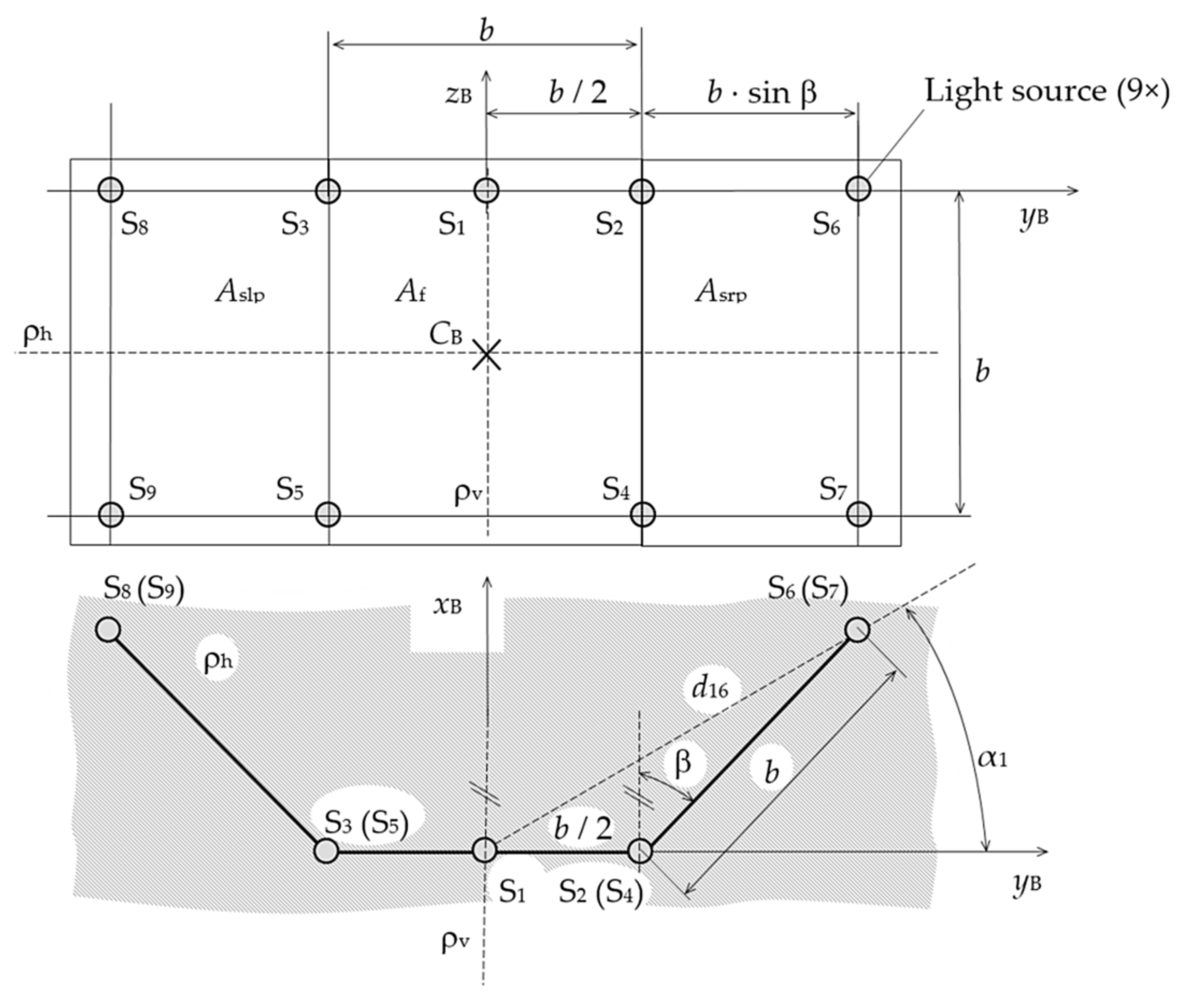
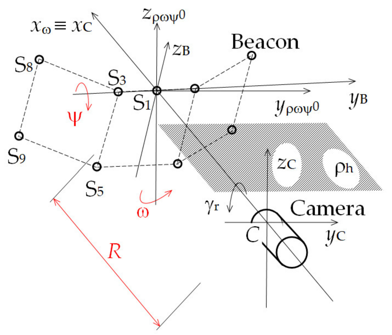
The above equations were derived assuming that the y_B beacon axis and y_C camera axis are parallel to the horizontal plane ρ_h (see Figure 2). Their mutual roll angle γ_r, which is created by the beacon or the camera rotation around the camera optical axis, was considered to be zero. The variables expressed with (2) to (5) are the functional distances R_i1 for diodes S_i, where i = 3, 5, 8, 9, and reference diode S₁. They are the beacon distances computed from the projections of the distances PS_i (between the reference diode S₁ and the functional diodes) onto the individual axes of the reference rectangular coordinate system and from the projections of the image distances b_i1 of these diodes onto transverse axes y_C and z_C of the camera coordinate system Cx_Cy_Cz_C. The reference coordinate system is parallel with the camera coordinate system. The axis x_ω of the reference coordinate system and the axis x_C of the camera coordinate system are identical with the camera optical axis. The origin of the reference system is at the intersection of the axis x_ω and the beacon front wall A_f (in the place of the reference diode S₁); the axes y_ρωψ0 and z_ρωψ0 lie in the plane ρ_ωψ0, which is identical with the beacon front wall A_f for ω = ψ = 0°. In this case, y_ρωψ0 ≡ y_B and z_ρωψ0 ≡ z_B. The azimuth and the elevation are formed by the beacon rotation around the axis z_ρωψ0 and y_B, respectively. Parameters d₁₆ and α₁ are derived from the beacon base b and the beacon opening angle β (see Figure 1). The working equations for the rest of the functional diodes are performed analogically. The elements PS_ixω are corrections of the deviation between the object distances of the functional diodes and the measured beacon distance.

For all the functional diodes, the rms of the functional distance differences D_rms (m) is as follows:

$$D_{\mathrm{rms}}=\sqrt{\frac{1}{8}\cdot {\displaystyle \sum _{\mathrm{i}=2}^9{D}_{\mathrm{i}1}^2}},$$

(6)

where D_i1 (m) is the functional distance difference D_i1 (m) for the diode pair S_i and S₁. It is given by the formula

$$D_{\mathrm{i}1}=R_{\mathrm{i}1}-R_{\mathrm{M}},$$

(7)

where $R_{\mathrm{M}}$ (m) is the mean of the calculated functional distances. This mean is expressed by the following formula:

$$R_{\mathrm{M}}=\frac{{\displaystyle \sum _{\mathrm{i}=2}^9{R}_{\mathrm{i}1}}}{8}.$$

(8)

Changing the azimuth and the elevation in the working equations of the mathematical model leads to changes in the mean of the calculated distances and the rms of the distance differences. Assuming that the input position angles are equal to the true azimuth and the elevation, the beacon parameters are set exactly according to the selected values, and the camera has a high resolution, we could theoretically expect the rms of the distance differences to be practically zero.

3. Experimental Test Results

Three basic experimental tests and several check tests were performed. Their aim was to verify the functionality of the created mathematical model and the suitability of the simultaneous analytical method for measuring the optical beacon distance, azimuth, and elevation. The beacon base b and its opening angle β were equal to 470 mm and 56.2°, respectively (see Figure 1). The beacon was placed on a positioning mechanism, which was put on the Thorlabs RBB12A rotation stage. The MOTICAM 1080 camera was used, having two lenses with different focal lengths. 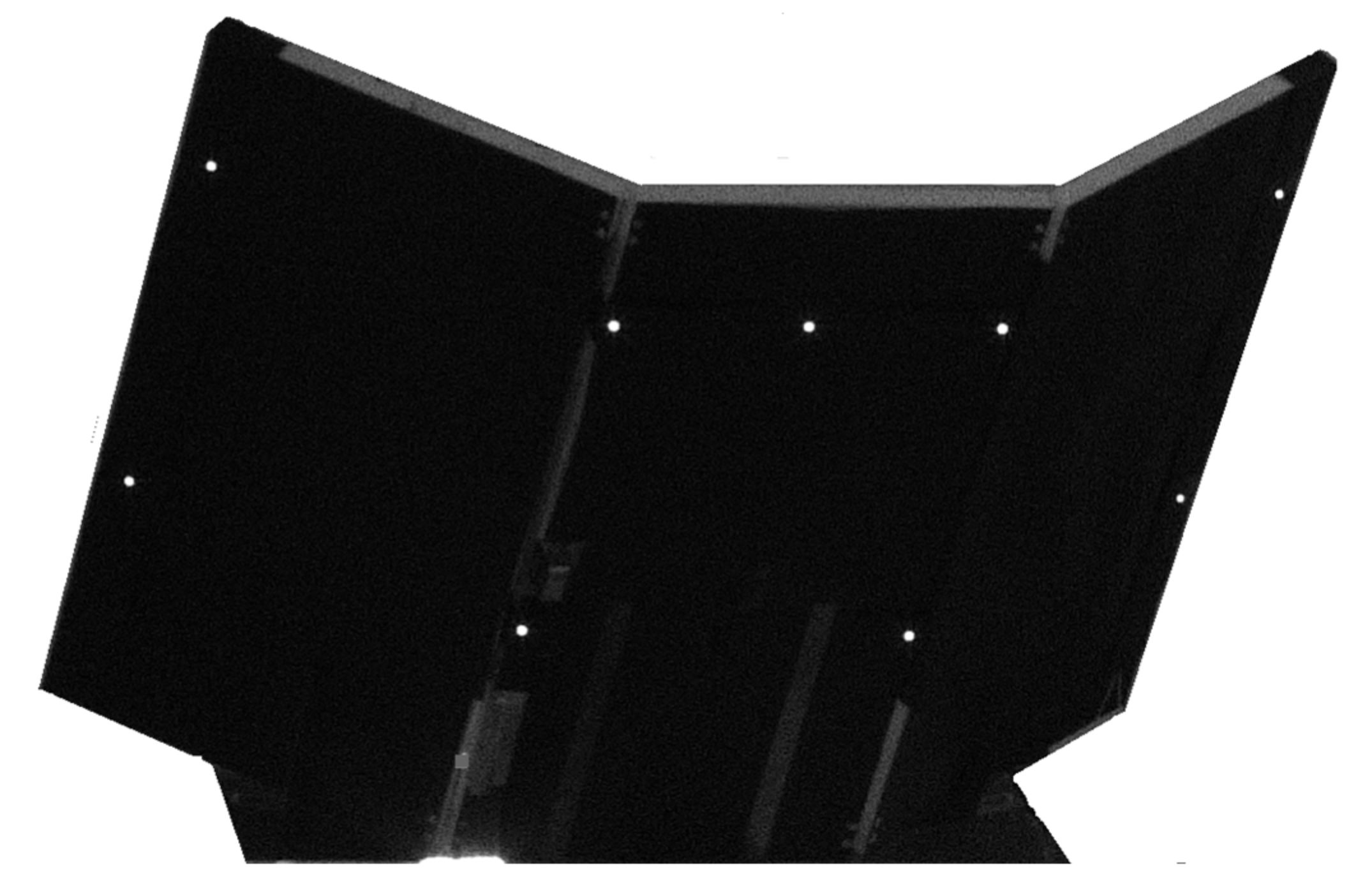Figure 3 shows beacon in the nominal position of ω_n = 20° and ψ_n = 35° during check test.

The rotation stage was used to set the actual beacon azimuth. The conventionally true azimuth ω₀ was measured using a scale of the actual rotation stage with the error of 2.5′. The azimuth nominal values ω_n were selected, around which the actual azimuth was set. The positioning mechanism was used to set the beacon elevation to nominal discrete values ψ_n in the range from 0 to 35° with the step of 5°. The conventionally true elevation values ψ₀ were measured using the Fortum model 4780200 inclinometer with the error of ±0.1°. The conventionally true beacon distances R₀ were measured using the Leica Disto D510 laser distance meter with the error of 1 mm. The nominal azimuth ω_n and elevation ψ_n were introduced to mark the groups of the conventionally true position angles as the azimuth was set randomly and, due to the random elevation of the relatively loose beacon fixation, the actual beacon elevation differed from the elevation set by the positioning mechanism.

The first experiment was performed using a lens with a focal length f_L = 120 mm. The beacon distance R₀ was 46,520 mm. The nominal azimuth ω_n (°) and elevation ψ_n (°) were {−3, 0, 3, 10, 20, 35, 46} and {0, 5, 20, 35}, respectively. For the individual nominal elevations, the azimuths were set around their nominal values and the beacon image was recorded. Five test series were performed for every elevation. Obtained results were used for statistical processing of errors. The second and third tests were performed with the same beacon, however, using a lens with a focal length f_L = 25 mm. The beacon distances were 13,460 and 46,728 mm, respectively. The setup of these tests was the same as for the first test. One hundred forty photos were taken for each distance and focal length; in total, 420 photos were taken.

Table 1. Nominal, conventionally true, and measured beacon position coordinates; first test.

Series		ωn (°)
		−3	0	3	10	20	35	46
1	Rm (mm)	46,407	46,457	46,486	46,588	46,708	46,875	46,858
	ψ0 (°)	21.6	21.6	21.6	21.5	21.5	21.3	21.2
	ψm (°)	21.3	21.5	21.5	21.3	20.8	20.5	21.1
	ω0 (°)	−3.3	0	3.5	10.3	19.8	35.0	45.8
	ωm (°)	−4.5	−1.1	2.2	9.1	18.7	33.8	44.8
2	Rm (mm)	46,402	46,472	46,474	46,553	46,733	46,974	46,931
	ψ0 (°)	21.6	21.6	21.6	21.5	21.5	21.3	21.2
	ψm (°)	21.4	21.1	21.1	20.8	20.8	20.5	21.1
	ω0 (°)	−3.3	0	3.4	10.3	20.0	35.00	46.1
	ωm (°)	−4.5	−1.3	2.2	9.0	18.8	33.7	45.0

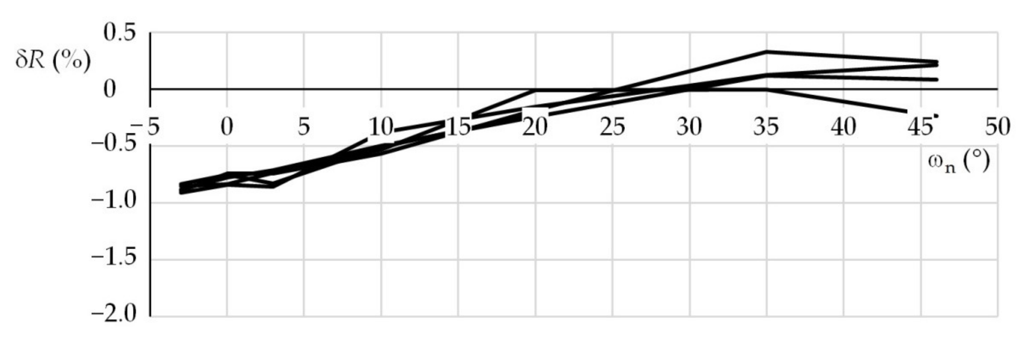
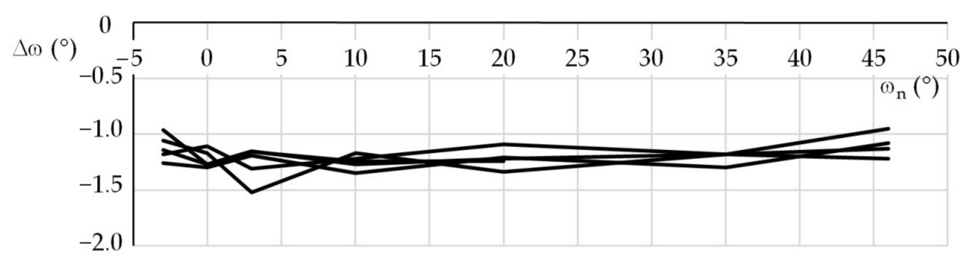
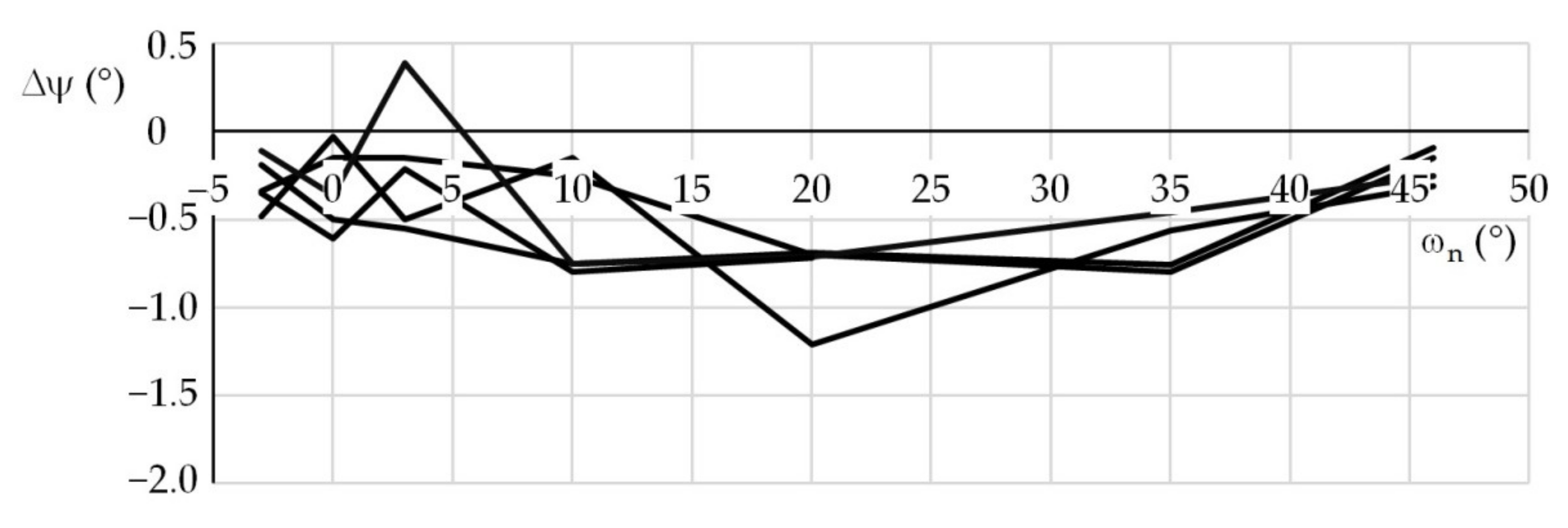
shows examples of distance R_m, azimuth ω_m, and elevation ψ_m that were measured during the first experiment in the first and second test series, for the nominal elevation of 20°. For comparison, the conventionally true values R₀, ω₀, and ψ₀ are also shown. Figure 4, Figure 5 and Figure 6 show the distance percentage errors δR and the position angles errors Δω and Δψ for the same test and in all the five test series.

The distance measurements from the first test were as follows: For the nominal elevation ψ_n = 0°, the mean of the measured distances $\overline{R}$ was 46,675 mm. For the nominal elevations of 5, 20, and 35°, the means of the measured distances were 46,668, 46,620, and 46,643 mm, respectively. Corresponding sample standard deviations s_R were 100, 127, 197, and 355 mm, respectively.

Results from the second experiment were as follows: For ψ_n (°) ∈ {0, 5, 20, 35}, the means of the measured distances were 13,513, 13,550, 13,518, and 13,499 mm. The corresponding sample standard deviations s_R (mm) ∈ {45, 45, 64, 105}.

From the measured distances in the third experiment, for the same above-mentioned nominal elevation, we yielded $\overline{R}\left(\mathrm{mm}\right) \{\mathrm{47,000}, \mathrm{46,933}, \mathrm{46,933}, \mathrm{46,925}\}$ and s_R (mm) ∈ {189, 129, 220, 374}. The presented values were determined from the test results of all five series.

The means and sample standard deviations of the distance percentage errors as well as azimuth and elevation errors, gained from the results of all three experiments, are listed in

Table 2. Summary of the distance measurement results.

	ψn (°)
	0	5	20	35
	fL = 120 mm, R0 = 46,520 mm, first test
$\overline{\mathsf{\delta }R} (\%)$	−0.31	−0.33	−0.43	−0.38
sδR (%)	0.21	0.27	0.42	0.76
FδR (%)	20/74/100	23/66/100	9/43/94	0/17/66
	fL = 25 mm, R0 = 13,460 mm, second test
$\overline{\mathsf{\delta }R} (\%)$	−0.39	−0.67	−0.43	−0.29
sδR (%)	0.33	0.33	0.48	0.78
FδR (%)	17/66/91	0/34/83	31/57/80	9/66/74
	fL = 25 mm, R0 = 46,728 mm, third test
$\overline{\mathsf{\delta }R}$ (%)	0.58	0.24	0.19	0.26
sδR (%)	0.40	0.28	0.44	0.80
FδR (%)	6/46/77	26/71/100	11/69/97	9/57/71

$\overline{\mathsf{\delta }R} (\%)$ is the mean percentage error of the distance. s_δR (%) is the sample standard deviation of the distance percentage errors. F_δR (%) is the frequency for absolute distance percentage errors 0.0 to 0.1%/0.0 to 0.5%/0.0 to 1.0%.

,

Table 3. Summary of the azimuth measurement results.

	ψn (°)
	0	5	20	35
	fL = 120 mm, R0 = 46,520 mm, first test
$\overline{\mathsf{\Delta }\mathsf{\omega }} (°)$	−1.55	−1.92	−1.20	−1.95
sΔω (°)	0.38	0.35	0.11	0.36
FΔω (%)	20/74/100	23/66/100	9/43/94	0/17/66
	fL = 25 mm, R0 = 13,460 mm, second test
$\overline{\mathsf{\Delta }\mathsf{\omega }}$ (°)	−4.1	−1.6	−1.8	−2.6
sΔω (°)	0.1	0.2	0.3	0.5
FΔω (%)	100/100/100	100/100/100	97/97/100	63/97/100
	fL = 25 mm, R0 = 46,728 mm, third test
$\overline{\mathsf{\Delta }\mathsf{\omega }}$ (°)	−2.0	−1.5	−1.8	−1.9
sΔω (°)	0.4	0.2	0.4	0.5
FΔω (%)	94/97/100	100/100/100	74/89/100	57/100/100

$\overline{\mathsf{\Delta }\mathsf{\omega }} (°)$ is the mean error of the azimuth. s_Δω (°) is the sample standard deviation of the azimuth errors. F_Δω (%) is the frequency for absolute azimuth errors 0.0 to 0.5°/0.0 to 1.0°/0.0 to 2.0°.

and

Table 4. Summary of the elevation measurement results.

	ψn (°)
	0	5	20	35
	fL = 120 mm, R0 = 46,520 mm, first test
$\overline{\mathsf{\Delta }\mathsf{\psi }} (°)$	−0.9	−1.0	−0.4	−0.2
sΔψ (°)	0.5	0.4	0.3	0.3
FΔψ (%)	20/54/100	9/49/100	57/91/94	77/100/100
	fL = 25 mm, R0 = 13,460 mm, second test
$\overline{\mathsf{\Delta }\mathsf{\psi }} (°)$	−0.6	−0.6	−0.4	−0.7
sΔψ (°)	0.4	0.4	0.3	0.6
FΔψ (%)	43/80/100	37/87/100	54/100/100	54/69/100
	fL = 25 mm, D = 46,728 mm, third test
$\overline{\mathsf{\Delta }\mathsf{\psi }}$ (°)	−0.8	−0.8	−0.3	−0.2
sΔψ (°)	0.9	0.5	0.4	0.6
FΔψ (%)	34/51/89	31/69/97	74/94/100	49/86/100

$\overline{\mathsf{\Delta }\mathsf{\psi }} (°)$ is the mean error of the elevation. s_Δψ (°) is the sample standard deviation of the elevation errors. F_Δψ (%) is the frequency for absolute elevation errors 0.0 to 0.5°/0.0 to 1.0°/0.0 to 2.0°.

. The measurement error frequency of these individual quantities is expressed in percentage from the total number of measurements for the individual nominal elevations. The intervals of the absolute distance percentage errors |δR| are 0.0 to 0.1%, 0.0 to 0.5%, and 0.0 to 1.0%. The spans of the absolute azimuth errors |Δω|and absolute elevation errors |Δψ|are 0.0 to 0.5°, 0.0 to 1.0°, and 0.0 to 2.0°.

The measured azimuth and elevation means and their sample standard deviations are not presented as their conventionally true values mostly differed from the nominal values and were not the same even in the individual test series.

For azimuth, the error frequency was determined for the error deviations between the individual tests and the mean error of the particular test series. The reason for selecting these deviations was the beacon’s random default position in relation to the rotation stage and in relation to the support base in the azimuth. These random positions manifested themselves as a component of systematic errors. The default position differed for the individual elevations as a result of the necessary manipulation with the beacon. Thus, the relatively large nonzero mean errors were proportional mainly to the magnitudes of the unspecified default position of the beacon.

The elevation error frequency was evaluated analogously to the distance errors, according to the differences between the conventionally true and the measured values. In fact, the unspecified beacon elevation did not shift the measurement errors too much outside the selected intervals that were expected for the frequency.

4. Sources of Errors

The measurement errors of the simultaneous analytical method had the following basic causes:

• Differences between the actual beacon and camera parameters and the parameters that were entered into the mathematical model;
• Inaccuracies in determining the diode picture coordinates;
• Aberration of the camera lens;
• Inaccuracies in determining the beacon and camera mutual position.

4.1. Differences between the Actual Beacon and Camera Parameters and the Mathematical Model Parameters

The beacon base, the opening angle, and the camera focal length are all used in the beacon mathematical model. If the actual real values differ from the values entered into the model, methodological measurement errors occur. In general, these errors occur in all three measured coordinates. This fact worsens the measurement accuracy; however, on the other hand, it enables adjusting the measuring system with its optimal beacon parameters for which the accuracy indicator is the best. By modifying the mathematical model parameters, all the measured quantities can be affected. Especially, manipulation with the focal length of the camera lens is important in the mathematical model. It enables optimizing the beacon distance measurement accuracy, and at the same time, it does not influence the beacon measured angles.

4.2. Inaccuracies in Determining the Diode Picture Coordinates

The influence of the pixel number error (pixel coordinate error) was tested on the mathematical model, based on the fifth series of the first experiment results, with the beacon elevation of 5°. The azimuth of 10° was selected.

For one beacon diode, the number of pixels was increased by one or by two for the y_C coordinate. Subsequently, the corresponding distance, azimuth, and elevation were determined. The influence of the pixel coordinates was tested for all nine diodes. The change of the measured beacon position was always measured only for the y_C pixel coordinate of one diode. The gained results are provided in

Table 5. Changes of measured angles when changing pixel coordinates.

Diode	yC0	zC0	yC0 + 1	Δωp1	Δψp1	yC0 + 2	Δωp2	Δψp2
1	1009	239	1010	0.3	0	1011	0.5	0.1
2	1230	242	1231	0	0.1	1232	0	0.3
3	789	236	790	0.1	−0.3	791	0.1	−0.5
4	1223	688	1224	0.1	−0.1	1225	0.1	−0.1
5	773	679	774	0.1	−0.1	775	0.1	−0.1
6	1578	225	1579	0	0	1580	−0.1	0.2
7	1566	668	1567	0	−0.2	1568	0	−0.4
8	363	202	364	0	−0.1	365	0	−0.2
9	350	649	351	0	0	351	0	0

.

Changes of the position angles Δω_p1, Δψ_p1 and Δω_p2, Δψ_p2 are the differences between the original azimuth and elevation and the new azimuth and elevation for the increased pixel coordinates y_C0 + 1 and y_C0 + 2, respectively, where y_C0 is the original pixel coordinate. A change of the pixel coordinate just in one direction can affect all three measured quantities. The distance deviations are not presented in Table 5 as they were only in order of hundredths of a percent. The maximum of the distance error changes was about 0.15%.

It is clear from the table that most deviations for both angles were in order of tenths of a degree. Their maximum magnitude was 0.3° for the change by one pixel and 0.5° for the change by two pixels. The deviations were zero in some cases. They occurred not only when the pixel coordinate was increased by one pixel, but also when the pixel coordinate was increased by two pixels. The nonzero deviations for two pixels were in most cases larger than deviations for one pixel. They were never smaller.

When the pixel coordinates changed for several diodes, the measured position angles changed by more than one degree. This was verified by the pixel coordinates being assessed by two persons independent of each other. The deviations of the determined pixel number were observable at both the y_C coordinates and the z_C coordinates. The biggest difference found between the measured position angles was 1.5°. It is clear that the method is sensitive to the accuracy of determining the pixel coordinates.

4.3. Lens Aberration

In general, camera lens aberrations can be the cause of measurement errors. The distortion of all the used lenses was experimentally verified. The distortions were not measurable. Other lens aberrations were compensated manually. For these reasons, the influence of the lens aberrations on the measurement accuracy was not considered.

4.4. Inaccuracies in Determining Mutual Position of the Beacon and the Camera

The azimuth measurement results were burdened with some systematic errors due to the fact that some components of the azimuth were not determined and included in the conventionally true values. These components were the beacon rotation relative to the rotation stage movable disk and the supporting base rotation that the rotation stage was placed on. Another factor that could adversely affect the measurement accuracy of both position angles was the mutual tilt of the camera and the beacon, i.e., a mutual roll of these objects around the camera’s optical axis (see Figure 2). Two check measurements were performed with the aim of quantitatively assessing the mentioned inaccuracies.

The first check measurement helped to assess the influence of the undetermined components of the azimuth. The beacon was set with a maximum azimuth deviation of approximately 1.0° towards the rotation stage movable disk. The measurements were performed for two nominal elevations of 0 and 35°. For each elevation, the supporting base was set for initial azimuths of −6.2, 0, and 6.2°. For each of these azimuths, several conventionally true azimuths were set on the rotation stage. The resulting absolute azimuth deviations, relative to the initial azimuths of the supporting base, did not exceed 0.9 and 0.6° for the nominal elevations of 0 and 35°, respectively. The measurement errors were comparable to the errors obtained from the basic experiments. It is clear that for practical use of this method, a firm fixation between the observed object and the measuring pattern has to be ensured.

The influence of the mutual tilt between the camera and the beacon was also measured at nominal elevations of 0 and 35°. For each elevation, their mutual tilt γ_r was set at −1.1, 0.0, and 0.9°. The error span and the maximum measurement errors are provided in

Table 6. Effect of the mutual tilt between the camera and the beacon.

ψn (°)	γr (°)			γr (°)
	0	−1.1	0.9	0	−1.1	0.9
	δDmax − δDmin (%)			|δD|max (%)
0	0.71	0.77	0.83	0.36	0.45	0.53
35	1.94	1.71	1.56	1.37	1.27	1.32
	Δωmax − Δωmin (°)			|Δω|max (°)
0	0.58	0.74	0.63	0.38	0.74	0.60
35	3.30	3.40	3.29	1.82	1.88	1.87
	Δψmax − Δψmin (°)			|Δψ|max (°)
0	1.7	2.7	1.4	1.2	1.5	1.4
35	1.2	2.1	0.8	0.9	1.4	1.0

. It shows that the mutual tilt between the camera and the beacon influences the measurement error magnitude. However, for the selected relatively small tilts, it demonstrated itself only by a small accuracy worsening. In some cases, the errors were even smaller for the nonzero tilt than for the zero tilt. This phenomenon can be explained by the difference between the beacon parameters used in the mathematical model and the actual beacon parameters.

4.5. Influence of the Mathematical Model

The errors resulting from determining inaccuracies of the pixel coordinates, as well as the beacon parameter inaccuracies, are also influenced by the mathematical model character, formed by a system of working equations. The equation’s core is represented by the ratios of the distance projections between the reference diodes and the functional diodes and the corresponding distance projections of the diode images. The object distances are expressed by trigonometric functions of the azimuth and elevations. Both the azimuth and the elevation are independent variables that are systematically changed until the required solution, based on the above-mentioned rule, is found (see Section 2). The coefficients and the initial angles in the working equations are taken from the beacon parameters. The differences between the parameters used in the mathematical model and the actual beacon parameters contribute to the systematic errors. These differences burden the measurement accuracy of the individual functional diodes to different extents, depending on the actual position angles. These mentioned parameter differences cause various functional distance differences, for all functional diodes.

Sizes of images are determined from the pixel coordinates of the corresponding diodes. Errors of the pixel coordinate determination play a significant role in the measurement errors of all the position coordinates. Minimum systematic errors are given by the size of one pixel as it determines elementary measurement uncertainty that cannot be reduced. A manifestation of this uncertainty depends on the picture size, beacon parameters, and measured position angles.

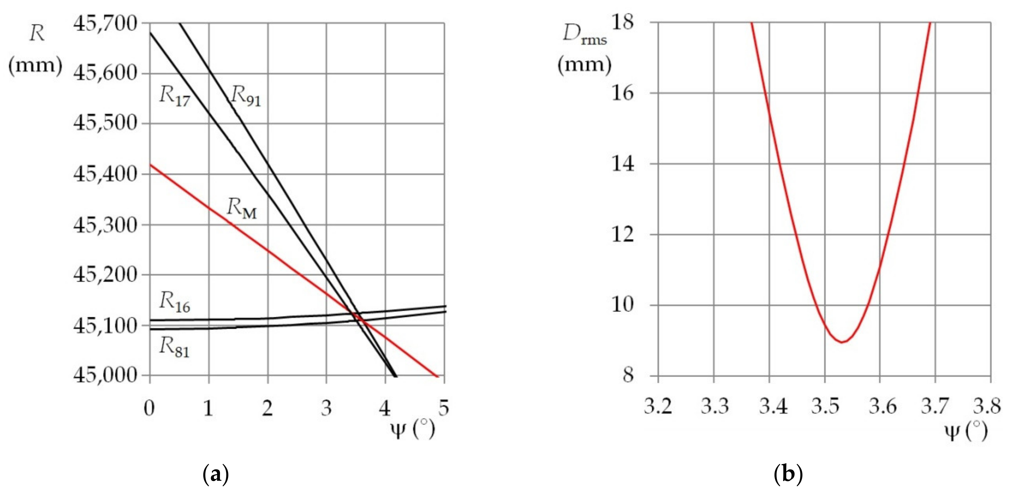
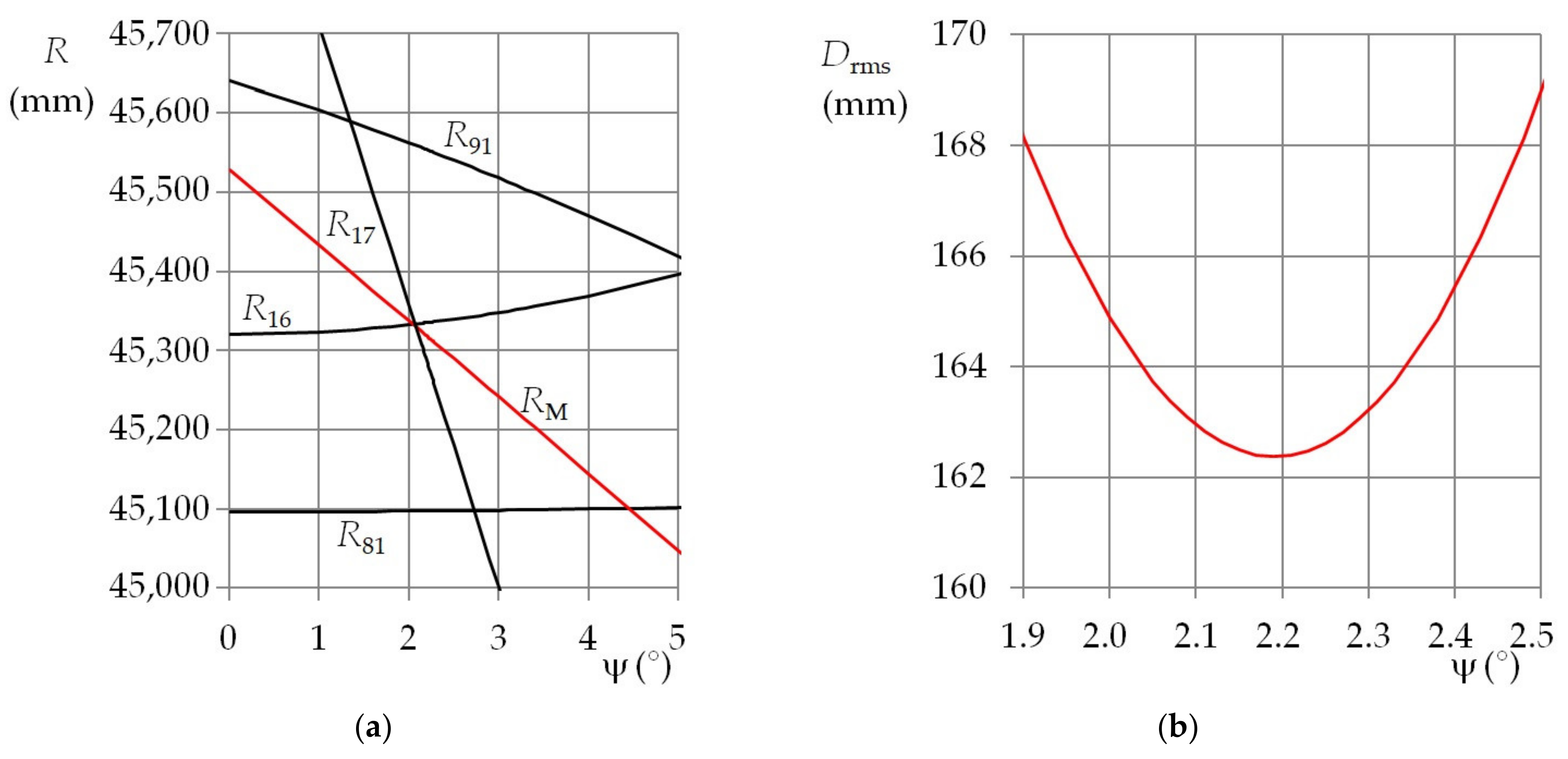
This fact is illustrated in Figure 7a and Figure 8a. They show the dependence of the functional distance, for the selected functional diodes, on the elevation that is entered into the mathematical model. Two combinations of the nominal position angles were used. Individual plots show azimuths when the rms minimum of the distance deviation D_rms was achieved. Due to the above-mentioned errors, the D_rms minimum had different levels for various combinations of the azimuth and the elevation. In addition, the rate at which the D_rms was approaching its minimum depended on the actual position angles. These properties are evident in Figure 7b and Figure 8b.

The presented results are from the first experiment (with beacon distance of 46,820 mm and a lens with focal length of 120 mm) for ω_n = ψ_n = 0° (see Figure 7a) and for ω_n = 20° and ψ_n = 0° (see Figure 8a). The plots show not only the functional distances R₁₆, R₁₇, R₈₁, and R₉₁ for the reference diode S₁ and the functional diodes S₆, S₇, S₈, and S₉, but also the calculated functional distance means R_M. In addition, the plots of the rms of the distance deviations D_rms for the mentioned diodes and the nominal position angles are shown in Figure 7b and Figure 8b. The functional distances are shown depending on elevation. The azimuth entered into the mathematical model was actually the parameter of the respective functions. The rms of the distance deviations was evaluated during the measurement process. Its only unambiguous minimum was determined using the entered azimuth and its appropriate elevation. By changing the azimuth, the minimum D_rms was shifted along the elevation axis and changed in size. Generally, a local minimum for a function with two variables was searched for. When the smallest rms was achieved, then the mean of the functional distances, the entered azimuth, and the appropriate elevation were the sought beacon coordinates.

It is clear from the plots of the functional distances that the measurement errors depend on the combination of the distance, azimuth, and elevation. If the measurements were burdened only with systematic errors, resulting from the incorrect determination of the actual position coordinates, the mean of the errors would be approximately constant. As the level of the random errors depended on the mentioned combination of the measured quantities, the mean errors expressed as a function of the azimuth often showed a certain trend—most often a significant local extreme (see Figure 4, Figure 5 and Figure 6).

This fact is clear from the functional distance plots. Each diode plot line has a different slope. If the slope is not steep, the deviations between the model parameters and the actual beacon parameters are the significant cause of the measurement errors. This applies especially to the beacon opening angle. It can happen that a small deviation of the beacon parameters has to be compensated by azimuths or elevations that differ very much from the actual values. If the slope of the functional distance line is steep, then the pixel coordinate errors will manifest for the image of the corresponding functional diode. As the distances between the images of the corresponding functional diodes and the reference diode are very small, the deviation of one or two pixels can cause big errors.

An important feature of the mathematical model is the fact that the pixel coordinate errors and the differences between parameters of the real beacon and the mathematical model do not have the same influence on the measurement errors. This is true in the whole range of the measured quantities and their combinations. Thus, the adjustment of the measuring system using optimization of the mathematical model parameters is possible only for some selected intervals of the measured quantities and their combinations. This mathematical model feature was especially apparent for the beacon opening angle.

5. Mathematical Model Adjustments

The influence of the beacon and camera parameters on the measurement results can be utilized for the adjustment of the mathematical model that contains all the relevant parameters. In general, it means that the measurement errors can be minimized by changing the system parameters in the mathematical model. As the errors are not linearly dependent on the measured quantities, the adjustment was performed using an optimization of the selected accuracy indicator. This indicator was selected from a group of results containing several combinations of the measured variables. The results were then compared with conventionally true values of the measured beacon position coordinates. Their high determining accuracy is the necessary precondition for successful adjustment. The measuring system can be adjusted using either the focal length or the beacon opening angle or the beacon base that manifests itself similarly to the focal length.

5.1. Mathematical Model Adjustment Using the Model Focal Length

Distance measurement errors can be reduced by selecting a suitable focal length f_M for the model (hereinafter model focal length). The position angle errors were affected by the focal length f_M only slightly. The focal lengths f_M entered into the model were 125.00 and 26.31 mm, where the actual real focal lengths f_L were 120 and 25 mm, respectively. The adjustment performed with the model focal length f_M is illustrated in

Table 7. Distance percentage errors δR (%) for different model focal lengths.

	ωn (°)
	−3	0	3	10	20	35	46
δR (%) for fM = 26.31 mm	−1.23	−1.11	−0.88	−0.75	−0.36	0.59	0.77
δR (%) for fM = 26.00 mm	−1.55	−1.21	−1.31	−0.69	−0.92	0.16	0.32
δR (%) for fM = 26.50 mm	0.34	0.70	0.59	1.20	0.99	2.05	2.26

for f_L = 25 mm, R₀ = 46,730 mm, and ψ_n = 35°. It is clear that small changes in the model focal length significantly affect the distance percentage errors.

Since the measured position angles remain almost constant while the model focal length is changing, the focal length f_M can be optimized by finding the minimum of the biggest distance percentage error for a random combination of the position angles in the provided beacon–camera configuration. The optimal focal lengths f_M were found for both beacon distances, performed with a lens with a focal length of 25 mm, and for two beacon elevations.

Table 8. Distance percentage errors δR (%) for the optimal model focal length.

	ωn (°)
	−3	0	3	10	20	35	46
	fL = 25 mm, R0 = 13,460 mm, ψn = 5°
δR (%) for fMo = fM13 = 26.15 mm 1	−0.40	−0.20	−0.10	0.03	0.04	0.35	0.42
	fL = 25 mm, R0 = 13,460 mm, ψn = 35°
δR (%) for fMo = 26.17 mm	−1.04	−0.85	−0.86	−0.62	−0.12	0.76	1.06
	fL = 25 mm, R0 = 46,730 m, ψn = 5°
δR (%) for fMo = fM46 = 26.19 mm 2	−0.37	−0.10	−0.07	−0.06	−0.17	−0.07	0.39
	fL = 25 mm, R0 = 46,730 m, ψn = 35°
δR (%) for fMo = 26.16 mm	−0.95	−0.60	−0.70	−0.10	−0.31	0.74	0.94

¹ The model focal length, which was determined as optimal for the beacon distance of 13,460 mm. ² The model focal length, which was determined as optimal for the beacon distance of 46,730 mm.

shows distance percentage errors for the optimal model focal length f_Mo.

Table 9. Errors for various optimal model focal lengths.

	ωn (°)
	−3	0	3	10	20	35	46
	fL = 25 mm, R0 = 13,460 mm, ψn = 5°
δR (%) for fM13 = 26.15 mm 1	−0.40	−0.20	−0.10	0.03	0.04	0.35	0.42
δR (%) for fM46 = 26.19 mm 2	−0.24	−0.05	0.06	0.20	0.20	0.50	0.60
	fL = 25 mm, R0 = 46,730 mm, ψn = 5°
δR (%) for fM13 = 26.15 mm 1	−0.52	−0.26	−0.22	0.20	0.30	0.20	0.20
δR (%) for fM46 = 26.19 mm 2	−0.37	−0.10	−0.07	0.06	0.17	0.07	0.39

¹ The model focal length, which was determined as optimal for the beacon distance of 13,460 mm. ² The model focal length, which was determined as optimal for the beacon distance of 46,730 mm.

shows the percentage errors for both beacon distances and for two model focal lengths f_M13 and f_M46, which were determined as the optimal lengths for the elevation of 5°. From the comparison of the individual optimal focal lengths and the corresponding distance percentage errors, it is clear that the utilization of only one model focal length can be regarded as acceptable, within the selected intervals of the measured distances and angles.

5.2. Mathematical Model Adjustment Using the Beacon Opening Angle

Adjustment of the mathematical model, by entering the beacon opening angle β_M into the model (hereinafter model opening angle), consists of position angle error evaluation for different angles β_M. As an example,

Table 10. Optimization of the model opening angle.

	βM (°)
	56.0	56.5	57.0	57.5	58.0	59.0	59.5	60.0	60.5	61.0	62.0	63.0	64.0
	ωn = 0°, ψn = 20°
Δω (°)	−1.11	−1.11	−1.11	−1.11	−1.11	−1.21	−1.21	−1.21	−1.21	−1.21	−1.31	−1.31	−1.41
Δψ (°)	1.45	1.45	1.35	1.25	1.25	1.15	1.05	1.05	0.95	0.95	0.85	0.75	0.65
PArms (°)	1.29	1.29	1.24	1.18	1.18	1.18	1.13	1.13	1.09	1.09	1.10	1.07	1.10
	ωn = 20°, ψn = 20°
Δω (°)	−1.69	−1.39	−1.19	−0.99	−0.69	−0.19	0.01	0.31	0.51	0.81	1.41	1.91	2.51
Δψ (°)	0.20	0.20	0.30	0.30	0.30	0.40	0.40	0.50	0.50	0.50	0.60	0.70	0.80
PArms (°)	1.20	0.99	0.87	0.73	0.53	0.31	0.28	0.42	0.51	0.67	1.08	1.44	1.86

shows the results for several angles β_M and two combinations of nominal azimuth and elevation, [ω_n; ψ_n] (°). These combinations were [0; 20] and [20; 20]. Results from the first series of the first experiment were used; the beacon distance and lens focal length were 46,820 and 120 mm, respectively.

For the model opening angles β_M (°) ∈ 〈56, 64〉 with the step of 0.5°, the azimuth and elevation errors were evaluated. For every β_M, the root mean square of the position angle error PA_rms was determined according to the following formula PA_rms = ((Δω)² + (Δψ)²)^0.5/2. Model opening angle β_M is considered optimal when the PA_rms is minimum. If the PA_rms is minimum for more different angles, then the beacon distance percentage error can be taken into consideration.

The model opening angle affects all the measured quantities. It can potentially be used to optimize the measurement of the position angles regardless of their distance errors. Distance errors can be minimized separately by optimizing the model focal length as all the model working equations are linearly dependent on the focal length. However, the adjustment of the mathematical model with the opening angle is not suitable as the optimum opening angles vary significantly with different values and combinations of the measured position angles (see Table 10). In the presented cases, the optimal angles were 63.0° for [0; 20] and 59.5° for [20; 20].

6. Conclusions

The results of the performed experiments show that the presented simultaneous passive method is usable not only for two coordinates, but also for three position beacon coordinates. In both cases, the mathematical model was based on lens equations of the lines connecting the individual functional diodes with the reference diode. Their functional distances were derived from these equations, depending on one or two beacon position angles. The task was solved numerically according to the rms of the difference between the individual functional distances and the mean of the functional distances. When the minimum of this rms was reached, then, the mean of the functional distances and the substituted values of the position angles were taken as the required results. The method can be used in practice to determine the mutual position of the beacon and camera with sufficient accuracy not only in the 2D plane, but also in 3D. The measurement accuracy was limited mainly by the camera resolution. In addition, the deviations between the real beacon parameters and the mathematical model parameters also have some negative influence on the measurement errors.

The particular reached measurement accuracy for the selected configurations was comparable between the individual experiments. The distance percentage errors were in the order of tenths of a percent. The mean errors and standard deviations of the azimuth and elevation errors were in order of tenths of an angular degree. An increase in the absolute mean azimuth errors above one degree was caused by systematic errors as a consequence of the undetermined components of azimuths (see Section 4.4).

The measuring system can be adjusted by a suitable selection of some mathematical model parameters. The effects of the model focal length f_M and the model opening angle β_M were verified. The accuracy of the beacon distance measurement can be favorably affected by the focal length f_M entered into the mathematical model. Thus, it is possible to effectively reduce the distance percentage errors and to find the optimal focal length f_Mo, usable within all the intervals of the individual measured quantities, while the influence on the azimuth and elevation remains negligible. On the contrary, the influence of the angle β_M is reflected in all the measured coordinates. Thus, the angle β_M is potentially suitable for the azimuth and elevation; however, its utilization in practice is not suitable as its optimal value depends on the current β_M value and on the position angle combinations.

Analogously, the minimum and the maximum measured beacon distances were affected by the beacon size as much as by the focal length. The layout of the functional diodes, and their mutual position with the reference diode, had influence mainly on the span of the measured position angles. All equations of the mathematical model could not be used when some diodes appeared in one line and were not distinguishable or visible. This situation occurred for large beacon distances or when the position angles exceeded their limits ω_l and ψ_l. The limits are clearly provided not only by the beacon layout but also, in general, by both position angles; for ψ = 0° the ω_l = β, and for ω = 0° the ψ_l = 90°.

The option to use this method, but with a smaller number of diodes, was verified too. Only five diodes were used in this model. The diode S₁ was used as a reference diode, and the diodes S₆, S₇, S₈, and S₉ were tested as the functional diodes (see Figure 1). It is clear from the results that the method was also suitable. However, it was necessary to select only diodes for which the azimuth and the elevation had opposite manifestations. In other words, the line projections between the diodes had to extend for some functional diodes and shorten for others. The resultant errors were comparable with errors listed in Table 5, Table 6 and Table 7.

The presented method is potentially suitable for measuring the position of a random known object. Both the functional and the reference points have to be defined on the surface of this object. In an ideal case, all of these points are visible in the camera pictures. Their images have to be clearly visible so that the distances between the reference point and the individual functional points in the pictures are measurable. Analogously, with this purpose-built beacon, the mathematical model of the object of interest has to contain equations including the line projections (between the reference point and the individual functional points) in the corresponding plane and the line images in the plane of the camera detector.