An AI-Application-Oriented In-Class Teaching Evaluation Model by Using Statistical Modeling and Ensemble Learning †


Abstract
:1. Introduction
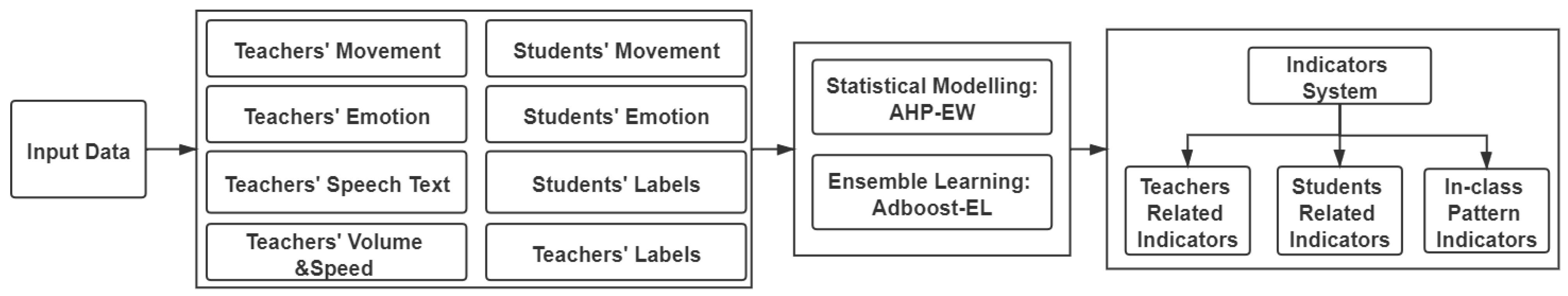
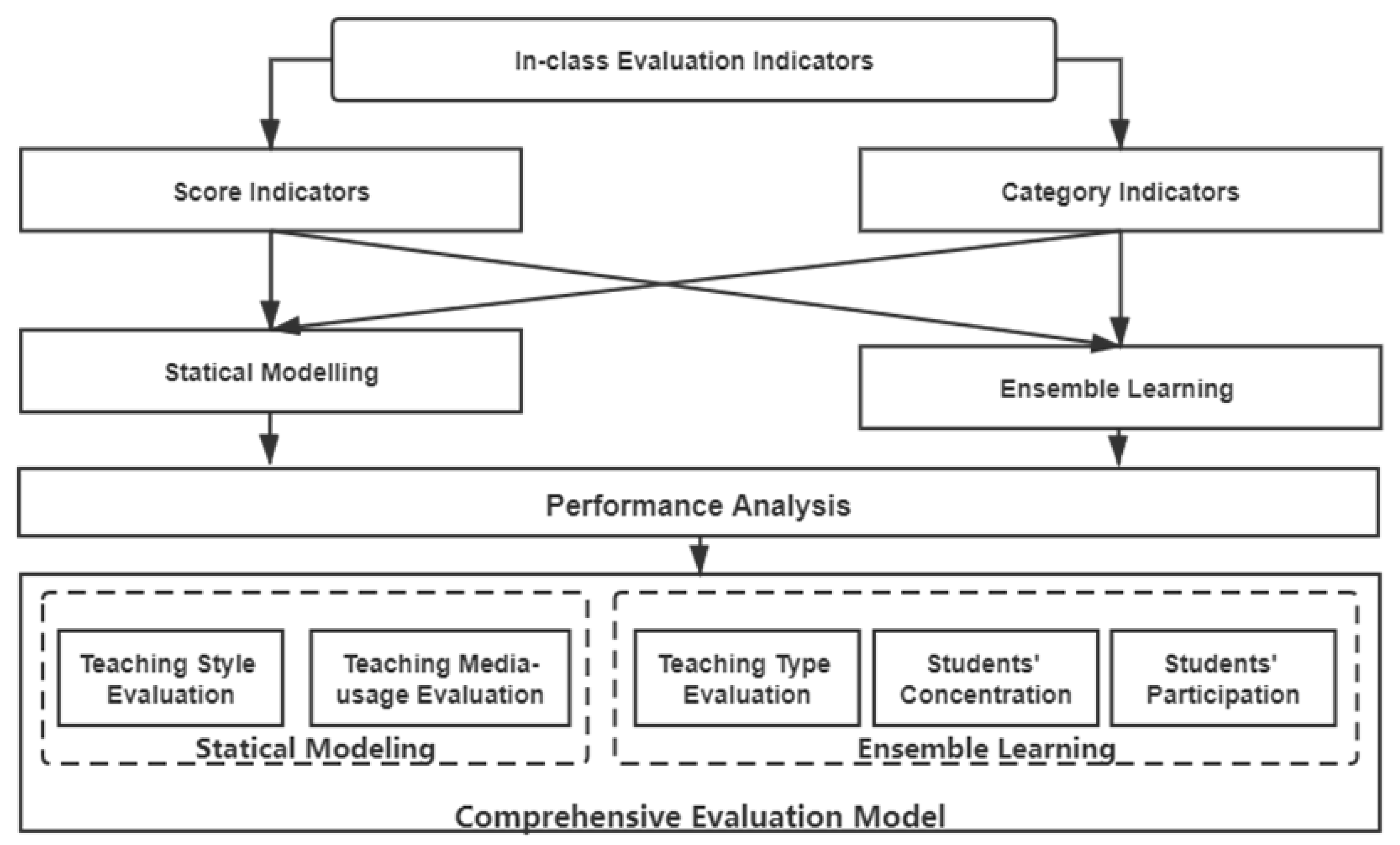
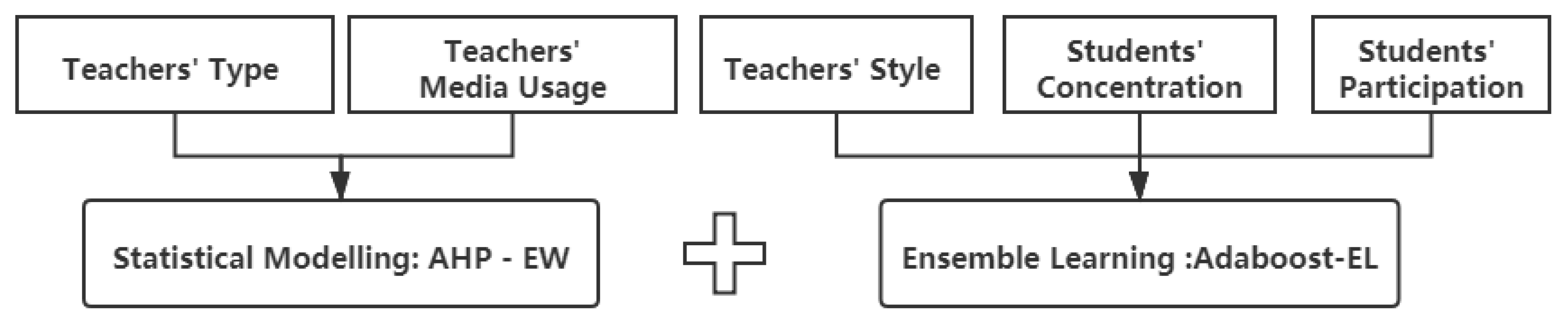
2. In-Class Evaluation Framework
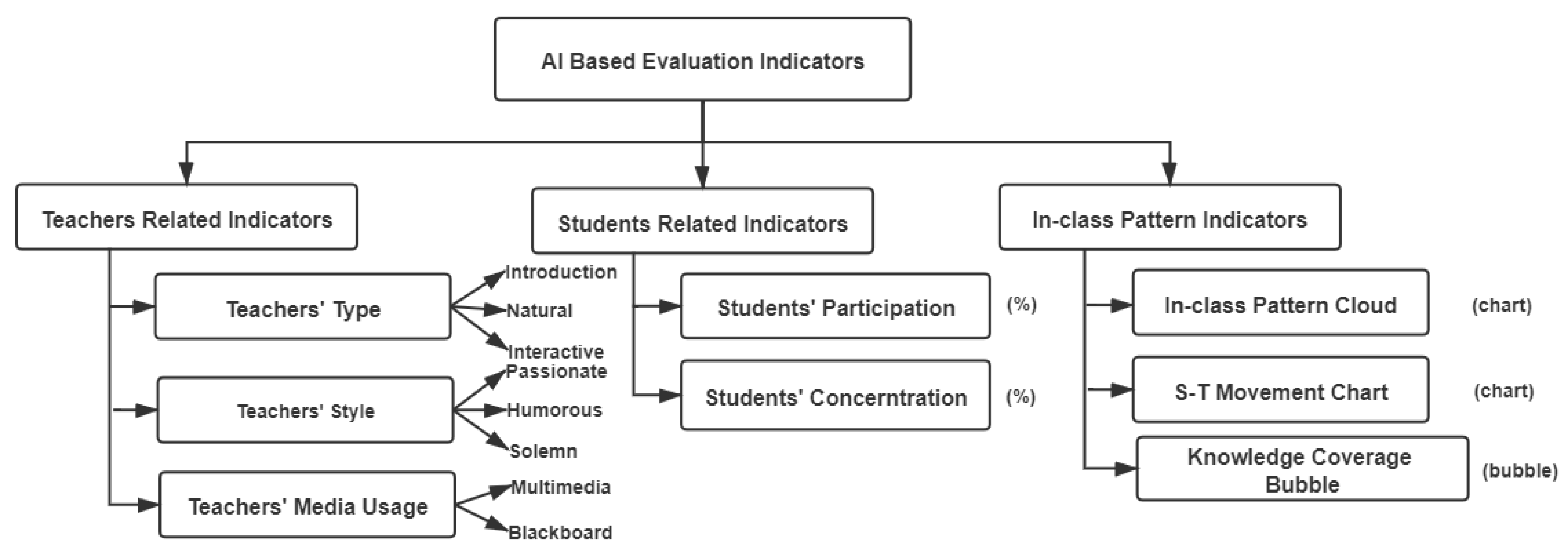
3. Index System Design
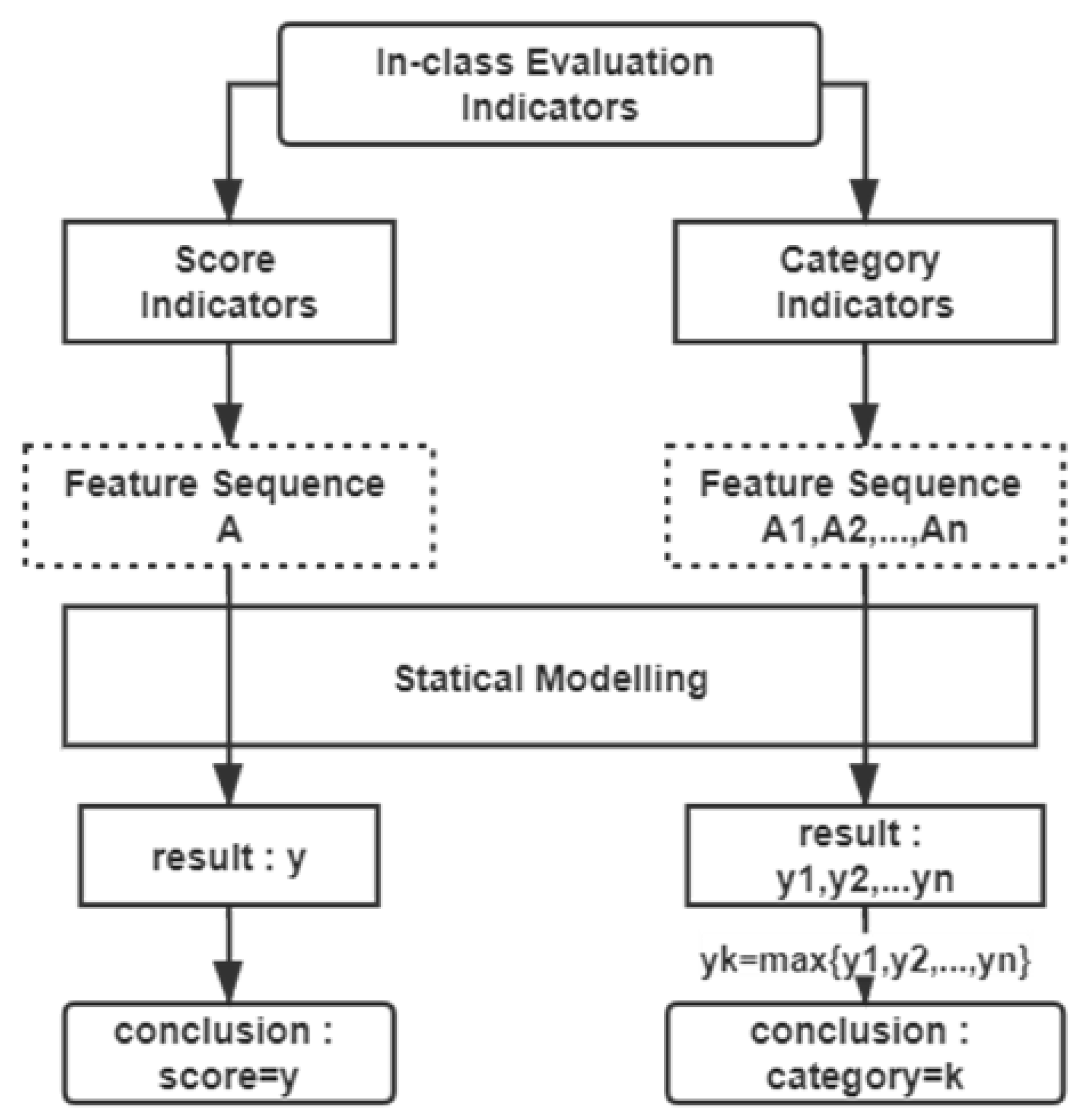
4. The Module of Statistical Modeling
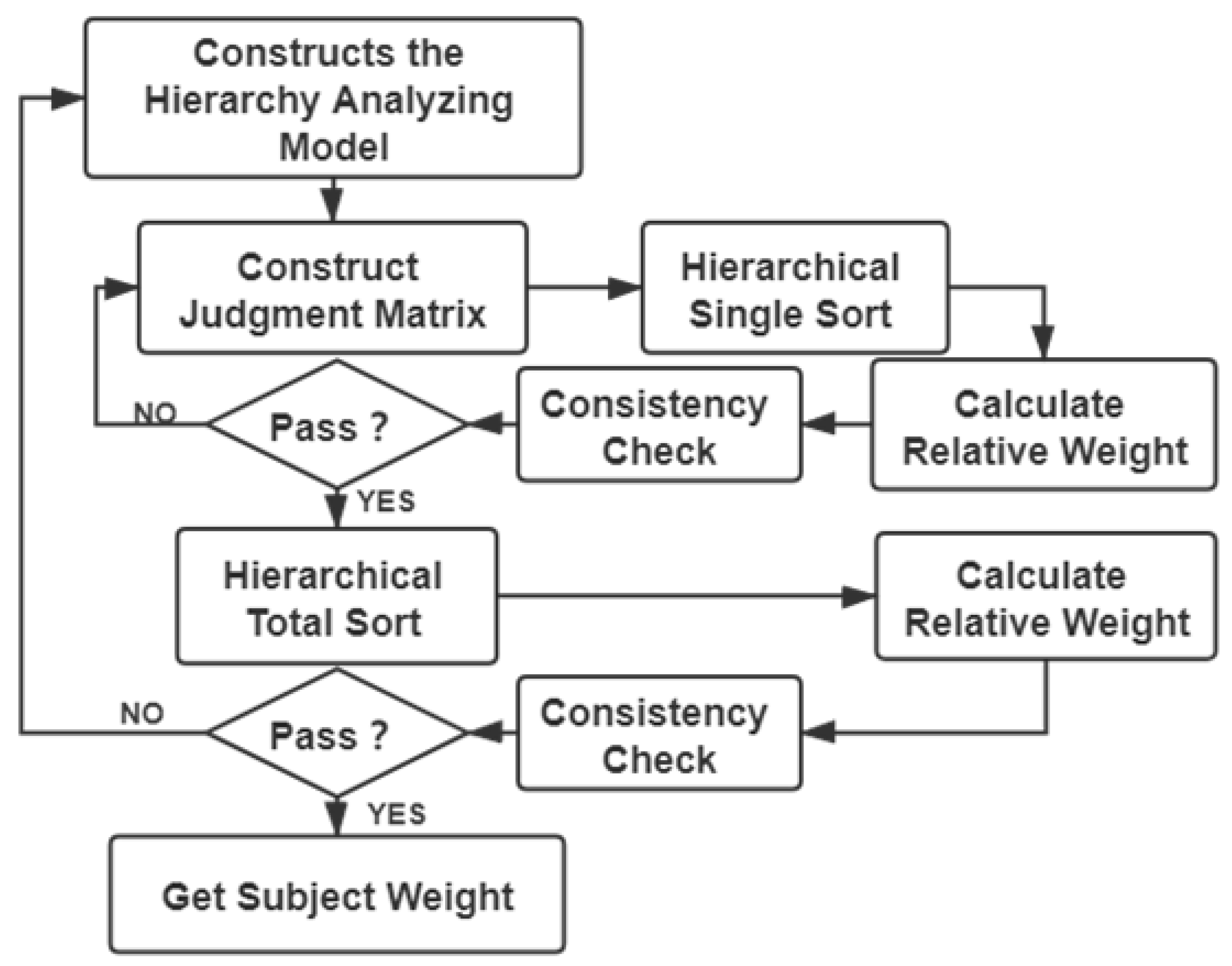
4.1. Analytic Hierarchy Process and Entropy Weight Method
- Build an analytic hierarchy model module,
- Construct a judgment matrix,
- Hierarchical ordering and consistency check,
- Consistency test and get subjective weight.
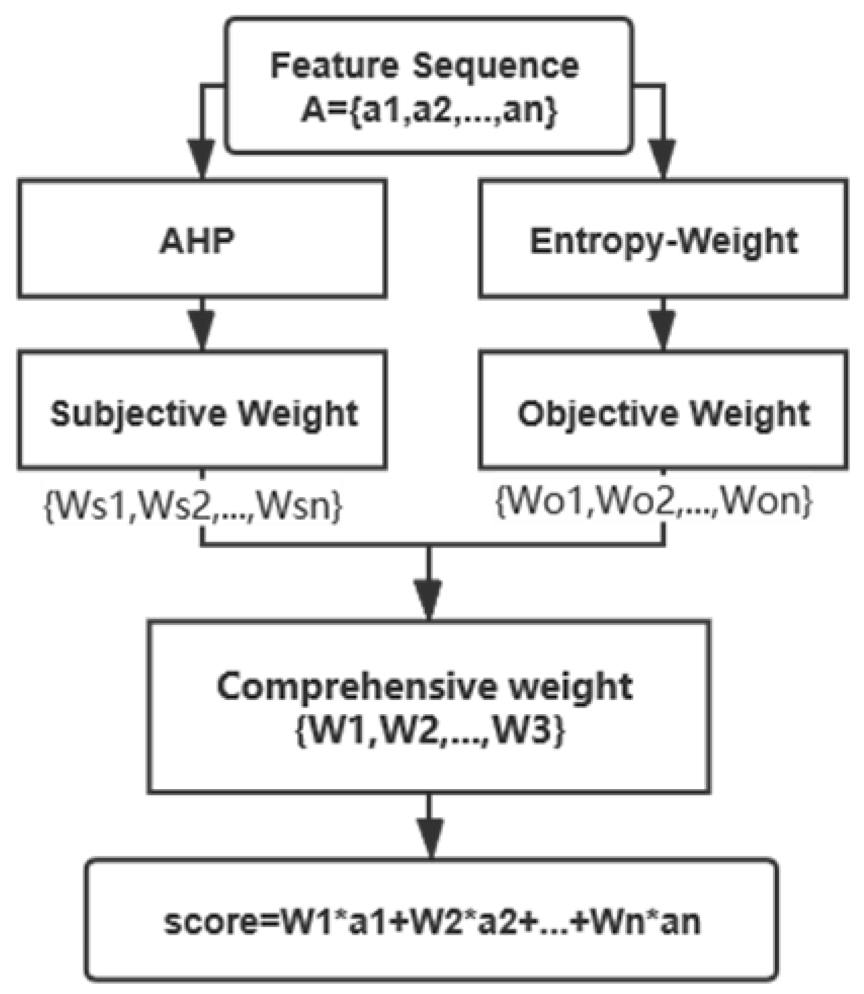
4.2. Analytic Hierarchy Process-Entropy Weight (AHP-EW) Statistical Modeling for In-Class Teaching Evaluation
- Step 1: Determine the type of indicators and find the corresponding feature sequence.
- Step 2: Calculate the subjective and objective weights of the features for the indicators.
- Step 3: Calculate comprehensive weights by the combination weighting optimization method.
- Step 4: Calculate each student sample’s final score of students’ concentration.
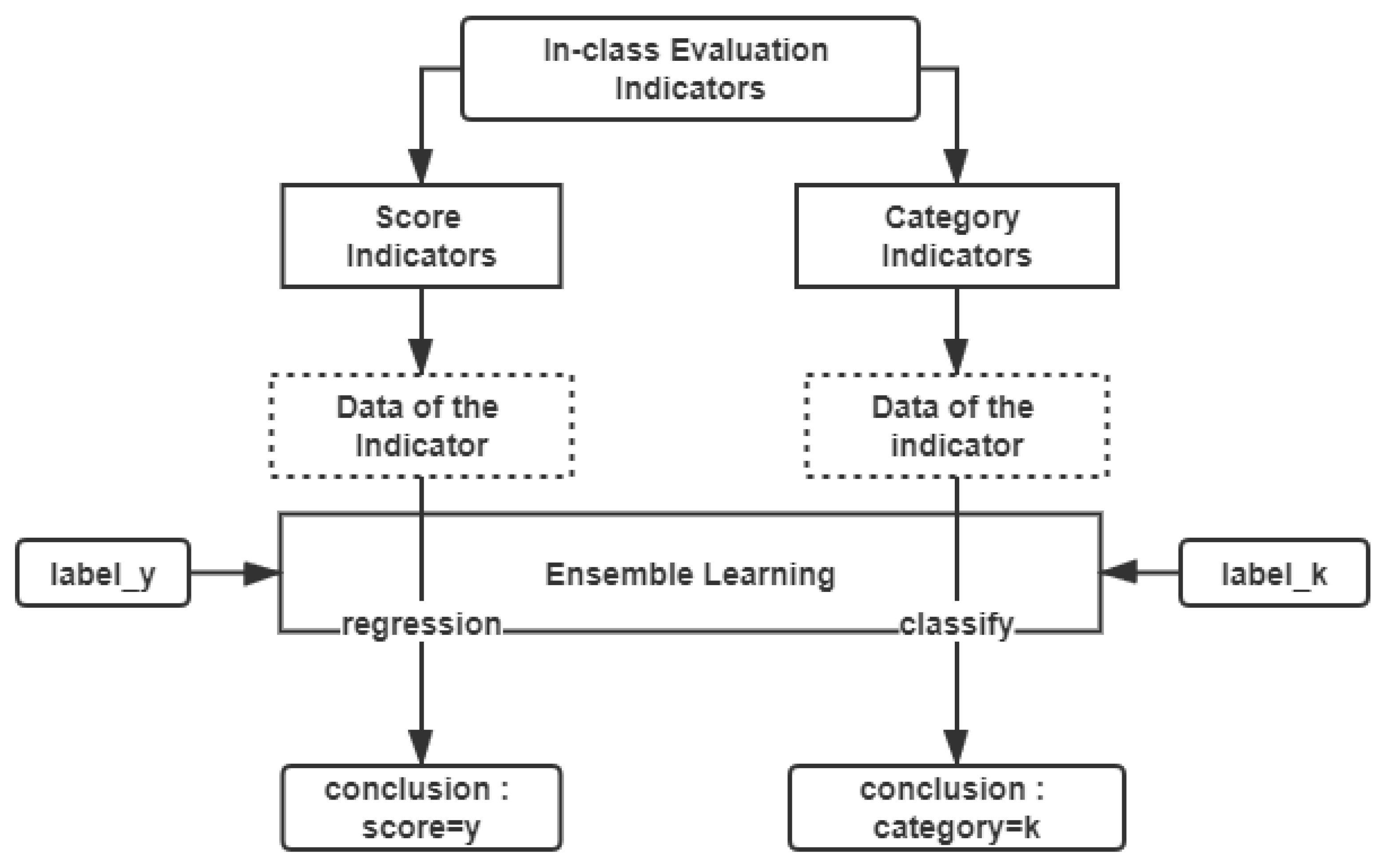
5. The Module of Ensemble Learning
5.1. AdaBoost
5.2. Adaboost-Ensemble Learning (Adaboost-EL) for In-Class Teaching Evaluation
- Step 1: Determine the type of the indicator and set the corresponding input data for ensemble learning module.
- Step 2: Construct the ensemble learning module and adjust its parameters.
6. Experiment and Performance Analysis
6.1. Input Data
6.2. Performance Analysis Indicators
- (1)
- Root mean square error (RMSE):
- (2)
- Accuracy (Accu.):
- (3)
- Confusion Matrix
- (4)
- Precision (P)
- (5)
- Recall (R)
- (6)
- F1_score (F1)
- (7)
- Macro_Precision (M_P)
- (8)
- Macro_Recall (M_R)
- (9)
- Macro_F-measure (M_F1)
6.3. Model Construction and Parameter Selection
6.3.1. The Example of Statistical Modeling Module
- Step 1: Determine the type of the indicator and find the corresponding feature sequence.
- Step 2: Calculate the subjective and objective weights of 11 features for students’ concentration
- Step 3: Calculate comprehensive weights by the combination weighting optimization method.
- Step 4: Calculate each student sample’s final score of students’ concentration.
6.3.2. The Example of Ensemble Learning Module
- Step 1: Determine the type of the indicator and set the corresponding input data for the AdaBoost-EL method.
- Step 2: Construct the ensemble learning module and adjust its parameters.
6.4. Performance Analysis
6.4.1. Performance Analysis of Statistical Modeling Module
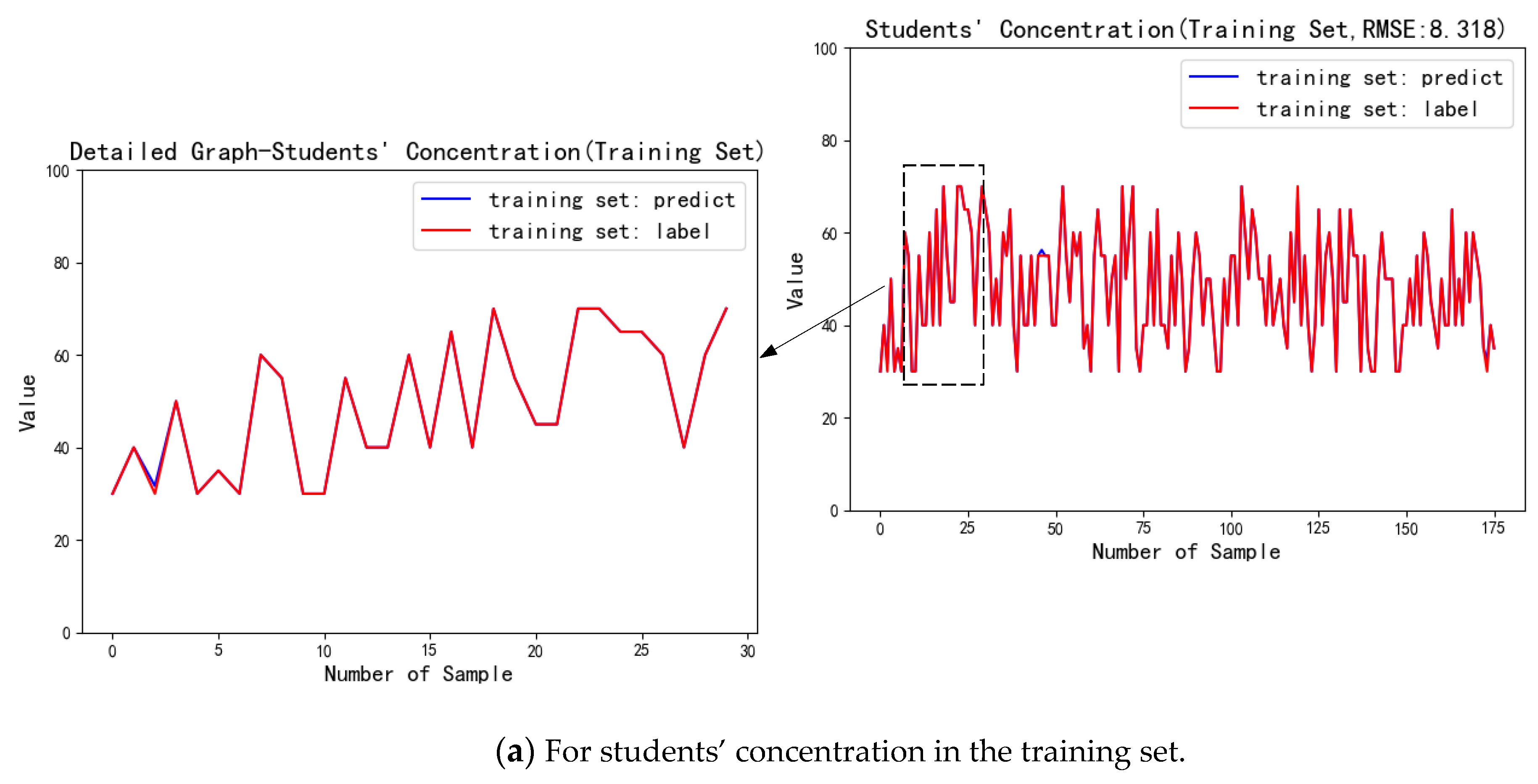
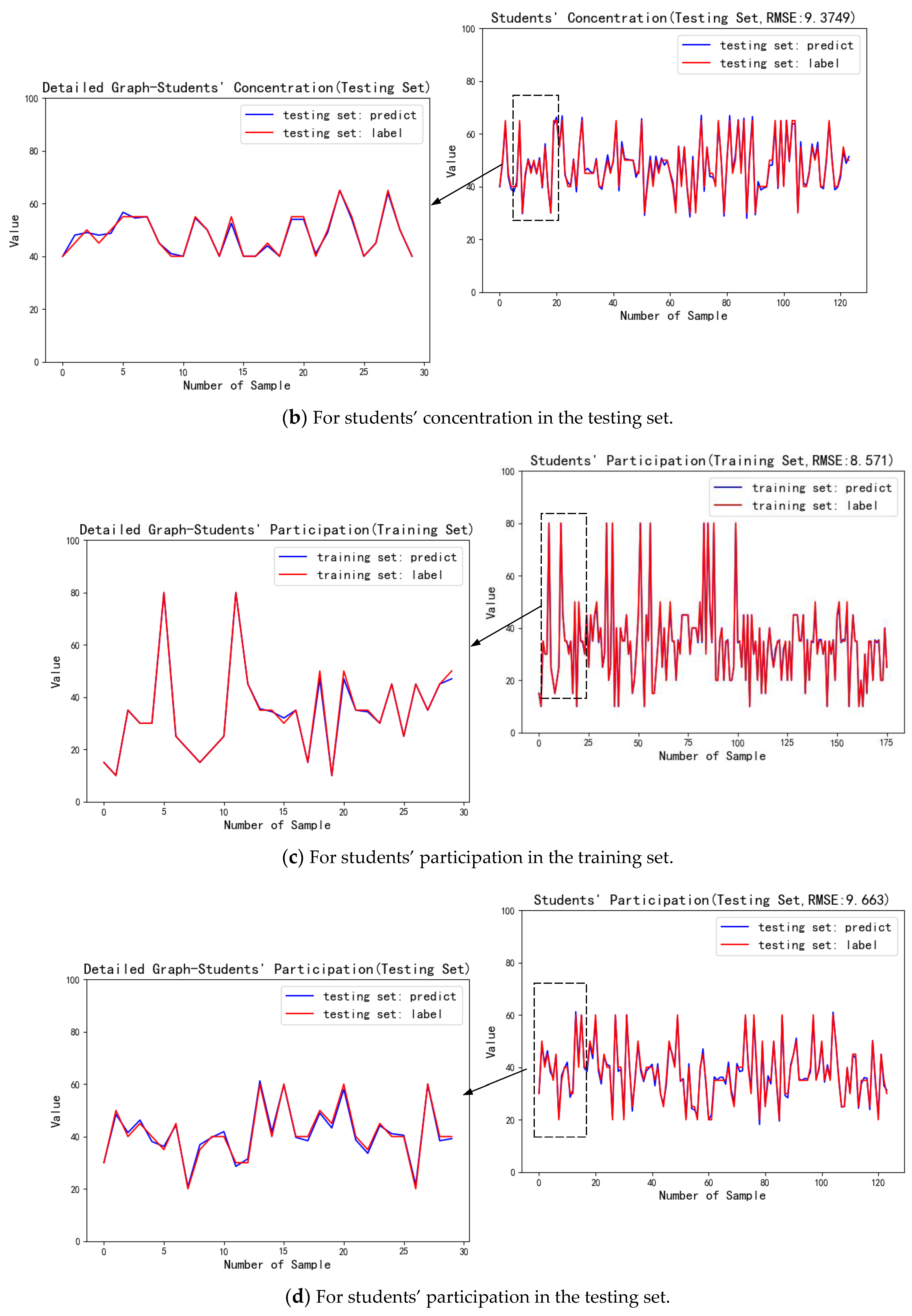
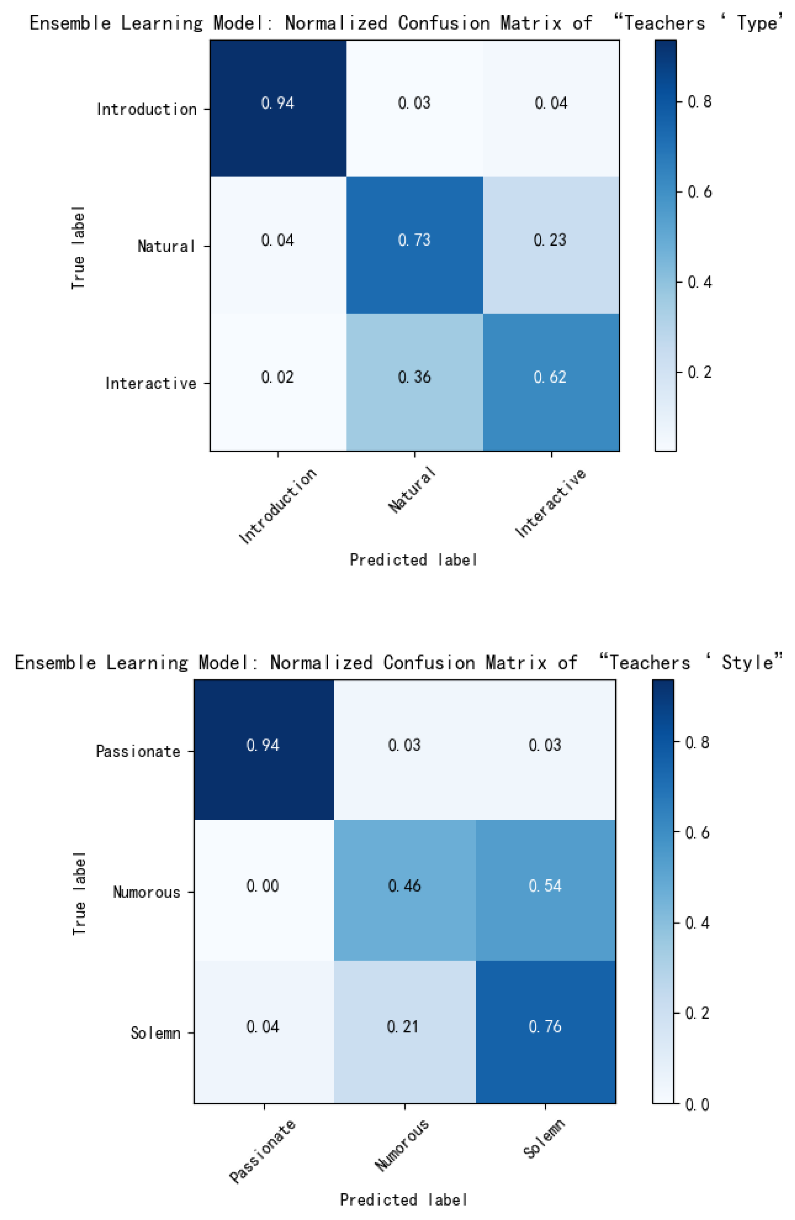
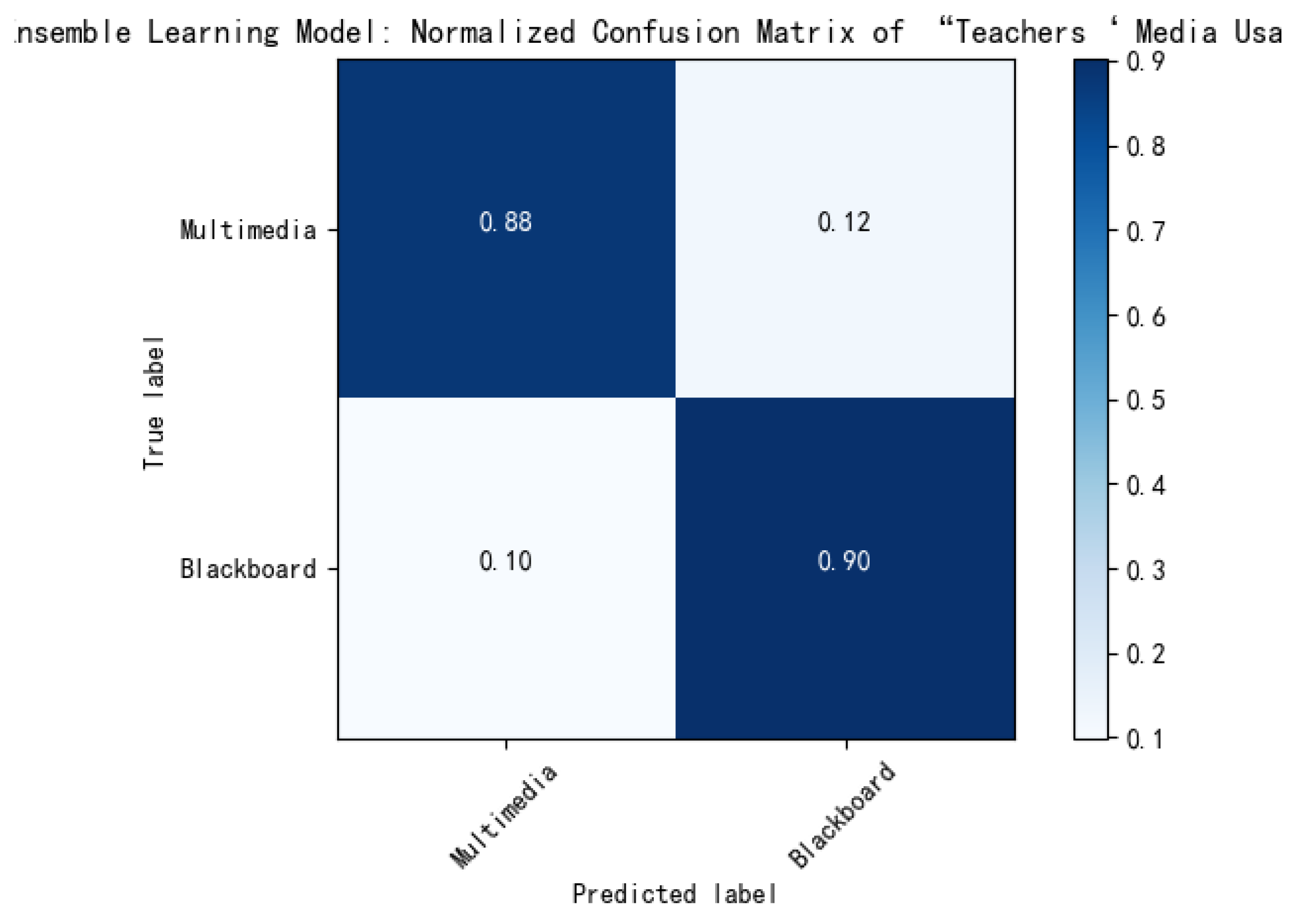
6.4.2. Performance Analysis of Ensemble Learning Module
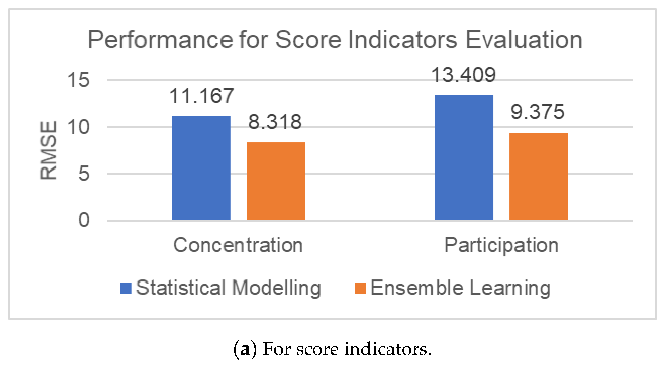
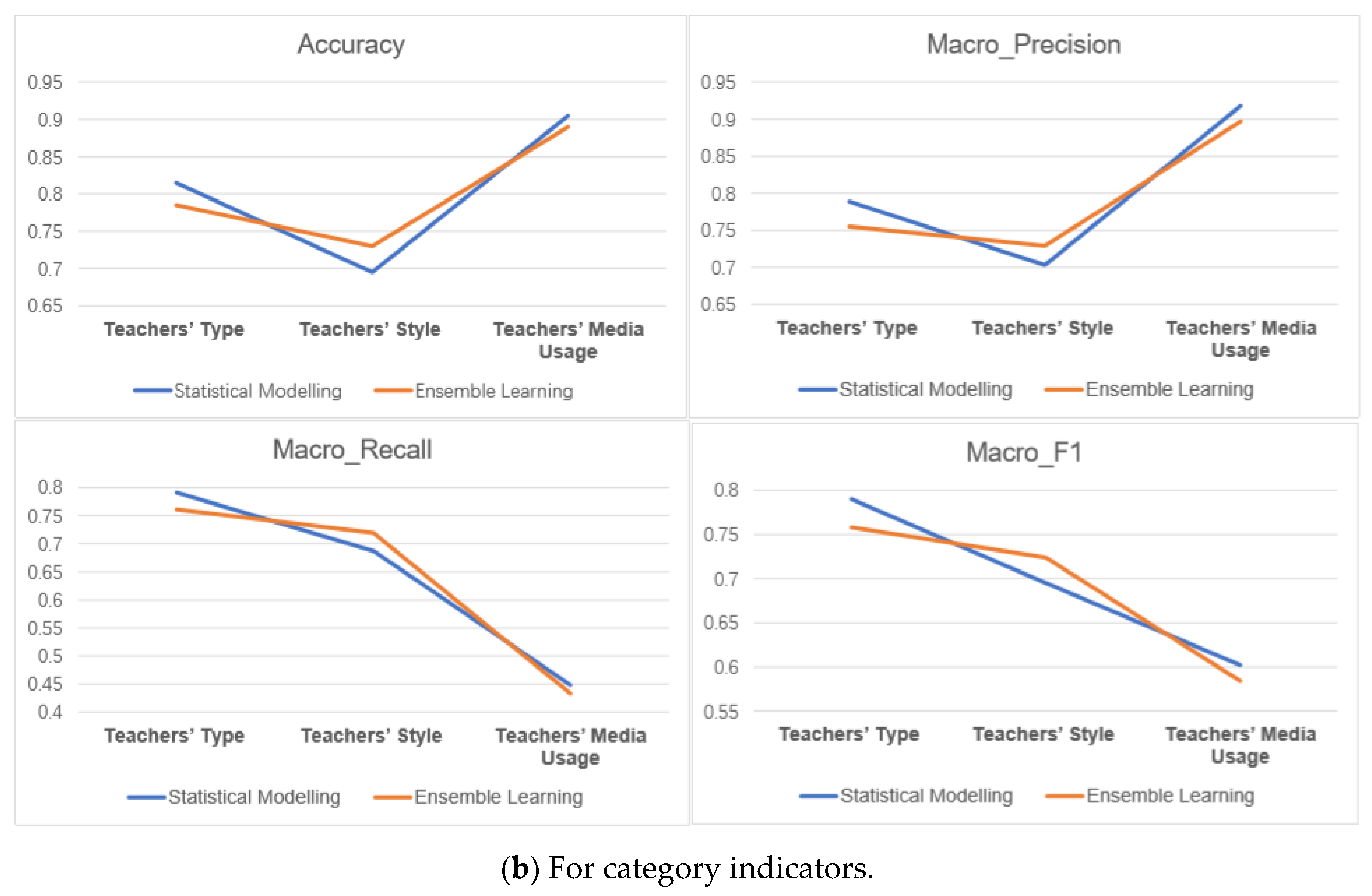
6.4.3. Comparison between the Two Modules
7. Conclusions
Author Contributions
Funding
Institutional Review Board Statement
Informed Consent Statement
Data Availability Statement
Acknowledgments
Conflicts of Interest
Appendix A
Appendix A.1.
| Algorithms A1 Calculating objective weights by the entropy weight method | |
| Input: For totally N samples and M corresponding features, the j-th feature value of the i-th sample ; | |
| Process: | |
| 1. | % Normalization of positive influence feature |
| 2. | % Normalization of negative influence feature |
| 3. , | |
| % Entropy value of the j-th feature | |
| 4. | % Information entropy redundancy of the j-th feature |
| end Output: Subjective weight of the j-th feature | |
Appendix A.2.
| Algorithms A2 Learning process of the AdaBoost algorithm | |
| Input:Dataset;; Basic-learner; Iteration; | |
| Process: | |
| 1. ; | % Initialize training set weight |
| 2. for : | |
| 3. | % use D and Dt to train the learner ht |
| 4. ; | % Calculate the error of learner ht |
| 5. if then break | |
| 6. ; | % Calculate the coefficient of learner ht |
| 7. | |
| 8. % Update the weight of training set, where Zt is the normalization factor. | |
| % | |
| 9. end | |
| Output: | |
Appendix B
| Device | Picture | Description |
| Real Classroom |  | Overall layout of the smart classroom |
| Pickup DS-2FP2020-A |  | To obtain the voice data in the classroom |
| Camera for students iDS-ECD8012-H/T (8–32 mm) |  | In the front of the classroom. To record the voice for students, and obtain the data such as students’ movement, emotion… |
| Camera for teachers iDS-EGD0288-HFR (8–32 mm) (2.8 mm) |  | In the middle of the classroom. To record the voice for teachers, and obtain the data such as teachers’ movement, emotion… |
References
- Wang, Y.; He, G. Inspirations and creativeness from the U.S. national education technology plan: Based on comparison and analysis of five U.S. national education technology plans (1996–2016). J. Distance Educ. 2016, 35, 11–18. [Google Scholar] [CrossRef]
- Ahmed, A.A.; Mona, R.A.; Abdel, H.S. Validating the modified System for Evaluation of Teaching Qualities: A teaching quality assessment instrument. Adv. Med. Educ. Pract. 2018, 9, 881. [Google Scholar]
- Andrejevic, M.; Selwyn, N. Facial recognition technology in schools: Critical questions and concerns. Learn. Media Technol. 2020, 45, 115–128. [Google Scholar] [CrossRef]
- Muramatsu, H. Trends of Technology Education in Compulsory Education in Japan. J. Robot. Mechatron. 2017, 29, 952–956. [Google Scholar] [CrossRef]
- Kim, H. An Exploratory Study on the Problems and Solutions of STEAM Education in Technology Education to Enhance STEAM Education. J. Korean Inst. Inf. Technol. 2016, 14, 211–218. [Google Scholar] [CrossRef]
- Best, M.; MacGregor, D. Transitioning Design and Technology Education from physical classrooms to virtual spaces: Implications for pre-service teacher education. Int. J. Technol. Des. Educ. 2017, 27, 201–213. [Google Scholar] [CrossRef]
- Ren, Y.; Zheng, X.; Wu, M. Promoting the Integration and Innovation of Information Technology with Education—Interpretation of China’s 13th Five-Year Plan for ICT in Education (2016). Mod. Distance Educ. Res. 2016, 5, 3–9. Available online: https://kns.cnki.net/kcms/detail/detail.aspx?FileName=XDYC201605002&DbName=CJFQ2016 (accessed on 1 January 2021).
- Youqun, R.E.N. Stepping into the New Age of Chinese Education Informatization: Interpretation of Education Informatization 2.0 Action Plan(1). e-Educ. Res. 2018, 6, 6. [Google Scholar]
- Gu, M.; Teng, J. China Education Modernization 2035 Framework and Its Significance for SDG4. Int. Comp. Educ. 2019, 5, 3–9, 35. Available online: https://kns.cnki.net/kcms/detail/detail.aspx?FileName=BJJY201905001&DbName=CJFQ2019 (accessed on 1 January 2021).
- Ye, L.I.; Dai, Q.H. On Exploration of University Supervisors in the Evaluation of Classroom Teaching Quality. In Proceedings of the 2018 International Conference on Education, Social Sciences and Humanities (ICESSH 2018), Chengdu, China, 25–26 March 2018; DEStech Publications: Lancaster, UK, 2018; pp. 24–27. [Google Scholar]
- Chen, Y.; Tao, T. The Design of Evaluation Index for Learning-oriented Classroom Teaching. Curric. Teach. Mater. Method 2016, 1, 45–52. [Google Scholar]
- Guo, Q. Exploring Teaching Evaluation in UC Berkeley. Tsinghua J. Educ. 2014, 5, 103–108. [Google Scholar]
- Wang, X. Multimedia Systems in Music Teaching of Normal University. In Proceedings of the 2011 International Conference of Environmental Science and Engineering (ICESE 2011 Part B), Singapore, 15 November 2011; Elsevier: Amsterdam, The Netherlands, 2011; pp. 535–539. [Google Scholar]
- Liu, Z.; Liu, Y. Teaching strategy and instructional system construction of Chinese national instrumental technology education. Eurasia J. Math. Sci. Technol. Educ. 2017, 13, 5645–5653. [Google Scholar] [CrossRef]
- Dai, Q.; Chen, Y.; Hua, G. Relationship between Big Data and Teaching Evaluation. In Proceedings of the 3rd International Conference on Education and Social Development (ICESD 2017), Xi’an, China, 8–9 April 2017. [Google Scholar]
- He, Y.; Li, T. A Lightweight CNN Model and Its Application in Intelligent Practical Teaching Evaluation. In Proceedings of the MATEC Web of Conferences, Sanya, China, 22–23 December 2019. [Google Scholar]
- Al_Janabi, S. Smart system to create an optimal higher education environment using IDA and IOTs. Int. J. Comput. Appl. 2020, 42, 244–259. [Google Scholar] [CrossRef]
- Flanders, N.A. Intent, Action and Feedback: A Preparation for Teaching. J. Teach. Educ. 1963, 14, 251–260. [Google Scholar] [CrossRef] [Green Version]
- Ogbu, J.U.; Feng, Z.; Yiqing, W. The purpose and method of Educational Anthropology. Abstr. Mod. Foreign Philos. Soc. Sci. 1988, 1, 44–45. [Google Scholar]
- Bei, L.; Qian, X.; Fang, L. Optimizing classroom observation by quantitative and qualitative methods. Surv. Educ. 2014, 15–17. [Google Scholar] [CrossRef]
- Yunfu, C. Classroom Observation: A New Par adigm. Res. Educ. Dev. 2007, 18, 38–41. [Google Scholar]
- Wu, J.; Lin, R.; Yu, X. Licc Mode of Classroom Observation: Lesson Set; Huadong Normal University Press: Shanghai, China, 2013. [Google Scholar] [CrossRef]
- Shirzadi, A.; Shahabi, H.; Chapi, K.; Bui, D.T.; Pham, B.T.; Shahedi, K.; Ahmad, B.B. A comparative study between popular statistical and machine learning methods for simulating volume of landslides. Catena 2017, 157, 213–226. [Google Scholar] [CrossRef]
- Han, Y.; Deng, Y. An evidential fractal analytic hierarchy process target recognition method. Def. Sci. J. 2018, 68, 367–373. [Google Scholar] [CrossRef] [Green Version]
- Kang, B.; Deng, Y.; Hewage, K.; Sadiq, R. Generating Z-number based on OWA weights using maximum entropy. Int. J. Intell. Syst. 2018, 33, 1745–1755. [Google Scholar] [CrossRef]
- Zhou, M.; Liu, X.B.; Yang, J.B.; Chen, Y.W.; Wu, J. Evidential reasoning approach with multiple kinds of attributes and entropy-based weight assignment. Knowl. Based Syst. 2018, 163, 58–75. [Google Scholar] [CrossRef]
- Xu, S.; Xu, D.; Liu, L. Construction of regional informatization ecological environment based on the entropy weight modified AHP hierarchy model. Sustain. Comput. Inform. Syst. 2019, 22, 26–31. [Google Scholar] [CrossRef]
- Li, G.; Li, J.; Sun, X.; Wu, D. Research on a Combined Method of Subjective-Objective Weighting Based on the Ordered Information and Intensity Information. Chin. J. Manag. Sci. 2017, 12, 179–187. [Google Scholar]
- Shafizadeh-Moghadam, H.; Valavi, R.; Shahabi, H.; Chapi, K.; Shirzadi, A. Novel forecasting approaches using combination of machine learning and statistical models for flood susceptibility mapping. J. Environ. Manag. 2018, 217, 1–11. [Google Scholar] [CrossRef] [PubMed] [Green Version]
- Norvig, P.; Russel, S. Artificial intelligence: A modern approach (all inclusive), 3/e. Appl. Mech. Mater. 1995, 263, 2829–2833. [Google Scholar]
- Sun, J.; Lang, J.; Fujita, H.; Li, H. Imbalanced enterprise credit evaluation with DTE-SBD: Decision tree ensemble based on SMOTE and bagging with differentiated sampling rates. Inf. Sci. 2018, 425, 76–91. [Google Scholar] [CrossRef]
- Schapire, R.E. The Strength of Weak Learnability. Mach. Learn. 1990, 5, 197–227. [Google Scholar] [CrossRef] [Green Version]
- Freund, Y.; Schapire, R.E. A Decision-Theoretic Generalization of On-Line Learning and an Application to Boosting. J. Comput. Syst. Sci. 1997, 55, 119–139. [Google Scholar] [CrossRef] [Green Version]
- Martin-Diaz, I.; Morinigo-Sotelo, D.; Duque-Perez, O.; Romero-Troncoso, R.D.J. Early fault detection in induction motors using adaboost with imbalanced small data and optimized sampling. IEEE Trans. Ind. Appl. 2017, 53, 3066–3075. [Google Scholar] [CrossRef]
- Bai, L.; Yu, Z.; Zhang, S.; Hu, K.; Chen, Z.; Guo, J. An In-class Teaching Comprehensive Evaluation Model Based on Statistical Modelling and Ensemble Learning. In Proceedings of the 4rd IEEE International Conference on Smart Internet of Things, Beijing, China, 14–16 August 2020. in press. [Google Scholar]


| Index | Input | Feature | Output |
|---|---|---|---|
| Students Concentration | Students’ Movement Students’ Emotion Concentration Judgment Matrix Concentration Labels | Frequency and Average Duration of 8 types of Students’ Movement; Frequency and Average Duration of 2 types of Students’ Emotion; | Score_Concentration |
| Students’ Participation | Students’ Movement Students’ Emotion Participation Judgment Matrix Participation Labels | Frequency and Average Duration of 8 types of Students’ Movement; Frequency and Average Duration of 2 types of Students’ Emotion; | Score_Participation |
| Teachers’ Type | Teachers’ Movement Teachers’ Emotion Teaching Type Labels | Frequency and Average Duration of 9 types of Teachers’ Movement; Frequency and Average Duration of 2 types of Teachers’ Emotion; | Score_ Indoctrination Score_ Natural Score_ Interactive |
| Teachers’ Style | Teachers’ Movement Teachers’ Emotion Teachers’ Volume and Speed Teaching Style Labels | Frequency and Average Duration of 9 types of Teachers’ Movement; Frequency and Average Duration of 2 types of Teachers’ Emotion; Mean and Variance od Teachers’ Volume and Speed | Score_Passionate Score_Humorous Score_Solemn |
| Teachers’ Media usage | Teachers’ Movement Media Usage Labels | Frequency and Average Duration of 9 types of Teachers’ Movement; | Score_ Multimedia Score_ Blackboard |
| Indicator | Input | Base Learners | Classification Algorithm | Output |
|---|---|---|---|---|
| Students’ Concentration | Students’ Movement Students’ Emotion Concentration Labels | Regression Tree | Forecast Score of Concentration | |
| Students’ Participation | Students’ Movement Students’ Emotion Participation Labels | Forecast Score of Participation | ||
| Teachers’ Type | Teachers’ Movement Teachers’ Emotion Teaching Type Labels | Classification Tree | SAMME | Types: Indoctrination, Natural, Interactive |
| Teachers’ Style | Teachers’ Movement Teachers’ Emotion Teachers’ Volume and Speed Teachers’ Style Labels | Types: Passionate, Humorous, Solemn | ||
| Teachers’ Media-usage | Teachers’ Movement Media Usage Labels | Types: Multimedia, Blackboard |
| Data Categories | Collection Methods | Data Content | |
|---|---|---|---|
| 200 teacher samples | Movement | Collect teachers’ movements per 3 s | Movement number (1–9) and corresponding time |
| Emotion | Collect teachers’ emotions per 3 s | Emotion numbers (1–2) and corresponding time | |
| Volume and Speed | Collect teachers’ volume (dB) and speed (word per minute) per 3 s | Volume value, speed value and corresponding time | |
| Speech Text | The content sequence of process speech text in the whole class | Every sentence and its start and end time | |
| Labels | Three evaluation labels marked by experts to evaluate the teachers from the courses. | Teaching type (1–3), Teaching style (1–3), Media usage (1–2). | |
| 300 student samples | Movement | Collect students’ movements per 3 s | Movement numbers (1–8) and corresponding time |
| Emotion | Collect students’ emotions per 3 s | Emotion numbers (1–2) and corresponding time | |
| Labels | According to the test after class and the Concentration and Participation in the whole class | Scores of the tests, Concentration and Participation in class |
| Predicted | Positive | Negative | |
|---|---|---|---|
| Actual | |||
| Positive | TP | FN | |
| Negative | FP | TN | |
| Subjective Weights and Orders | Objective Weights and Orders | Comprehensive Weights and Orders | |||||
|---|---|---|---|---|---|---|---|
| (1) | (2) | (3) | (4) | (5) | (6) | (7) | (8) |
| Feature | Weights | Orders | Weights | Orders | Reasonable Value Range | Weights | Orders |
| X1 | 0.166 | 1 | 0.072 | 7 | [0.072–0.166] | 0.121 | 2 |
| X2 | 0.142 | 3 | 0.109 | 4 | [0.109–0.142] | 0.125 | 1 |
| X3 | 0.094 | 6 | 0.062 | 10 | [0.062–0.094] | 0.080 | 8 |
| X4 | 0.031 | 10 | 0.071 | 8 | [0.031–0.071] | 0.053 | 11 |
| X5 | 0.151 | 2 | 0.043 | 11 | [0.043–0.151] | 0.095 | 5 |
| X6 | 0.140 | 4 | 0.102 | 5 | [0.102–0.140] | 0.120 | 3 |
| X7 | 0.106 | 5 | 0.075 | 6 | [0.075–0.106] | 0.088 | 6 |
| X8 | 0.041 | 8 | 0.069 | 9 | [0.041–0.069] | 0.056 | 10 |
| X9 | 0.032 | 9 | 0.133 | 1 | [0.032–0.133] | 0.083 | 7 |
| X10 | 0.023 | 11 | 0.132 | 3 | [0.023–0.132] | 0.073 | 9 |
| X11 | 0.074 | 7 | 0.133 | 2 | [0.074–0.133] | 0.105 | 4 |
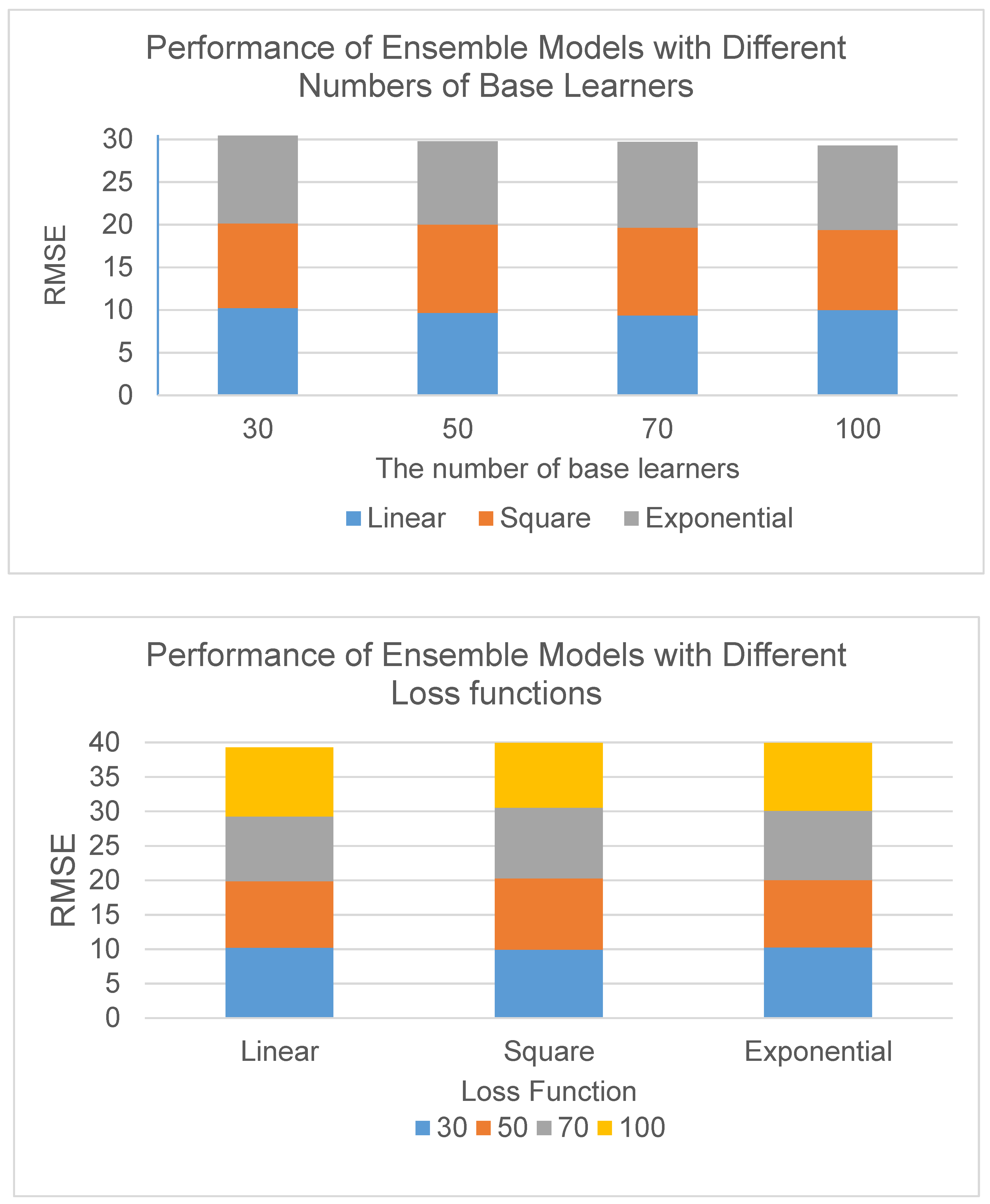
| Loss Function | The Number of Base Learners | RMSE |
|---|---|---|
| Linear | 30 | 10.2316 |
| 50 | 9.6649 | |
| 70 | 9.3749 | |
| 100 | 10.0136 | |
| Square | 30 | 9.9312 |
| 50 | 10.3445 | |
| 70 | 10.1863 | |
| 100 | 9.3807 | |
| Exponential | 30 | 10.2625 |
| 50 | 9.7782 | |
| 70 | 10.0313 | |
| 100 | 9.8675 |
| Statistical Modelling | Score Indicator | RMSE |
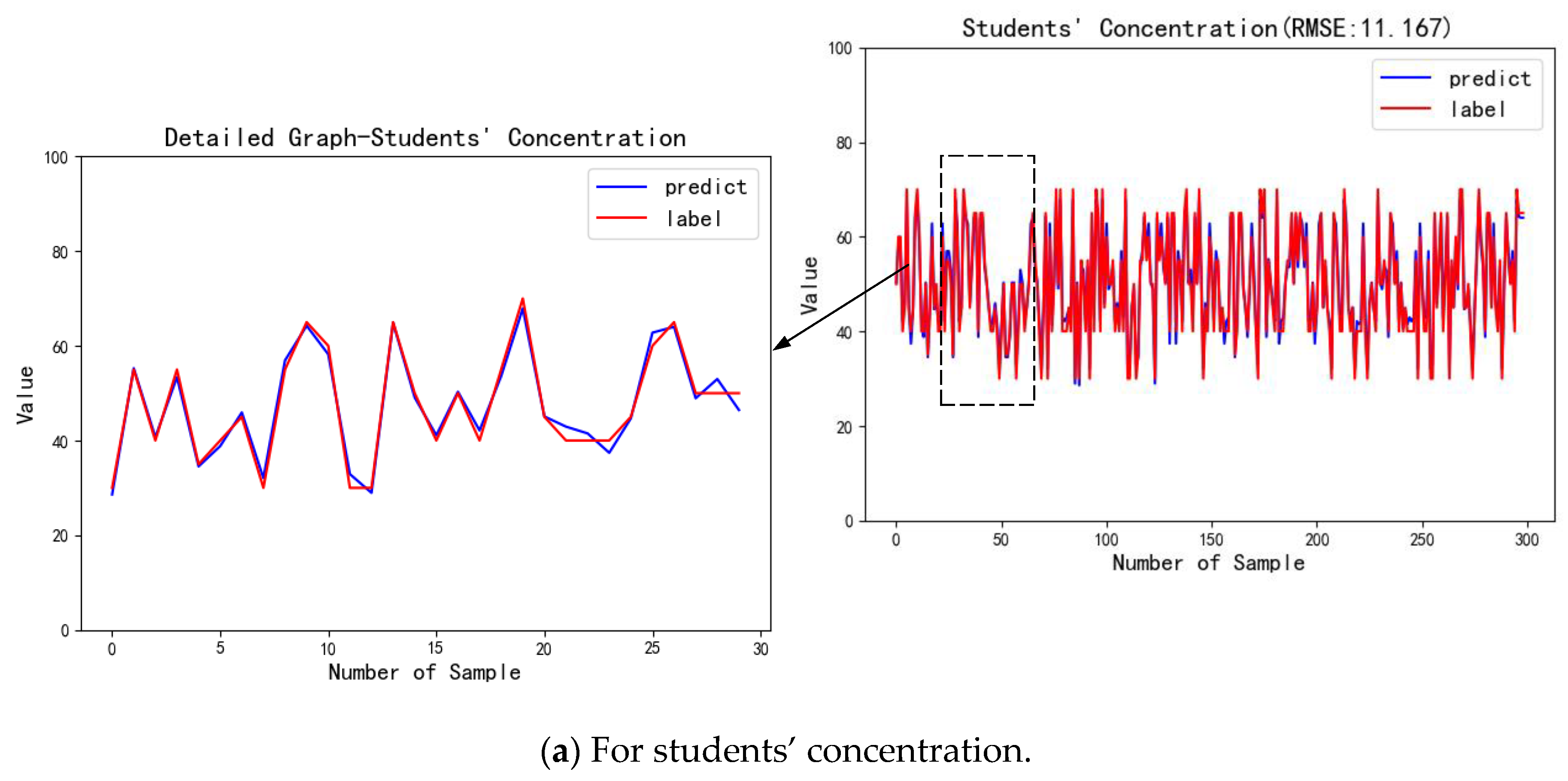
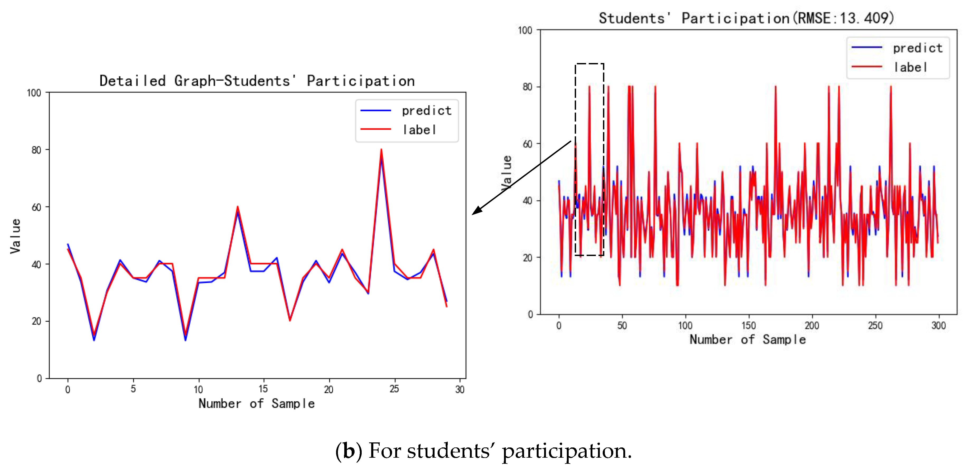
| Concentration | 11.167 | |
| Participation | 13.409 |
| Statistical Modelling | Category Indicators | Precision | Recall | F1 | Accuracy | M_P | M_R | M_F1 | |
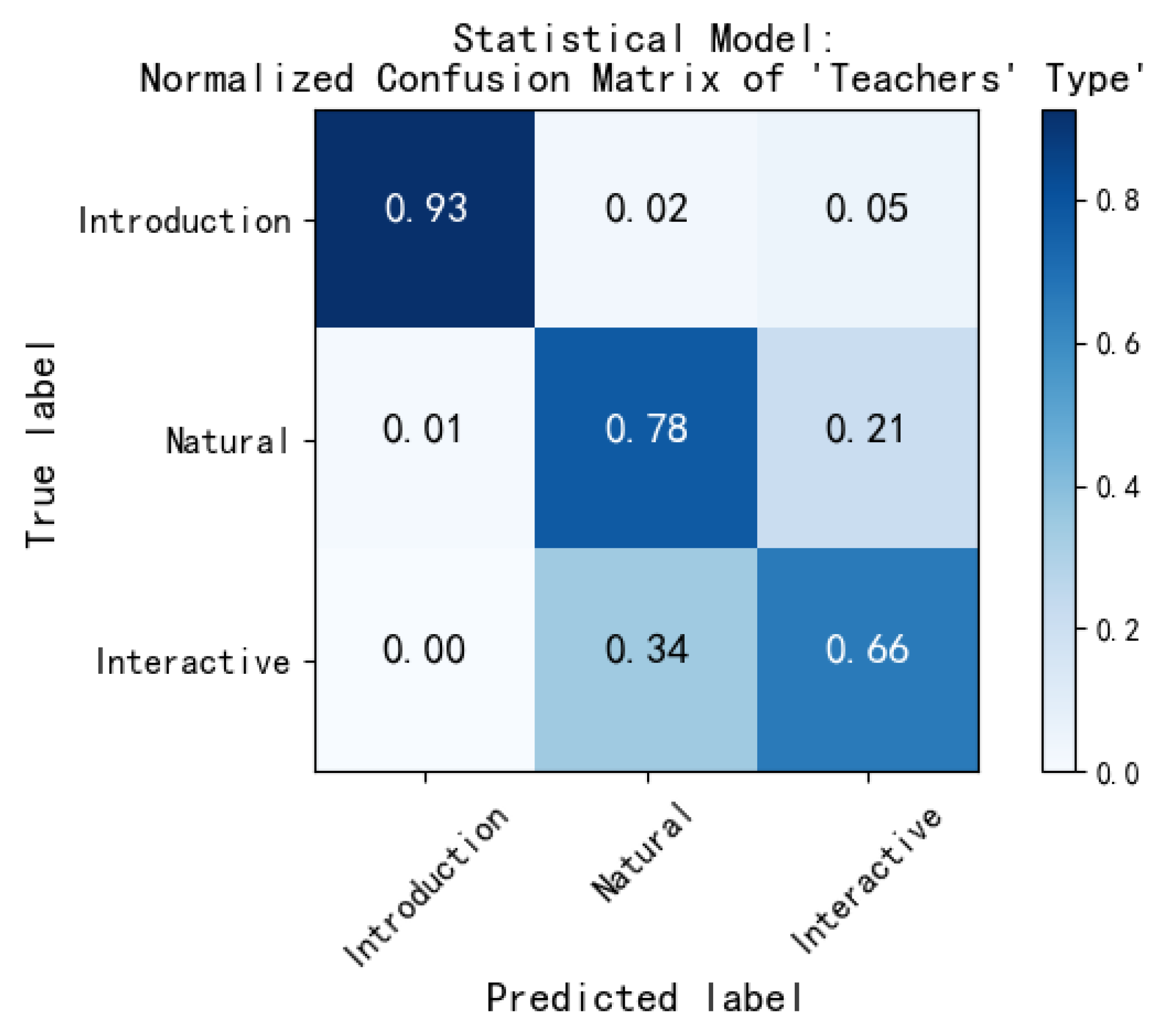
| Teachers’ Type | Indoctrination | 0.987 | 0.938 | 0.962 | 0.815 | 0.789 | 0.791 | 0.790 | |
| Natural | 0.776 | 0.776 | 0.776 | ||||||
| Interactive | 0.604 | 0.659 | 0.630 | ||||||
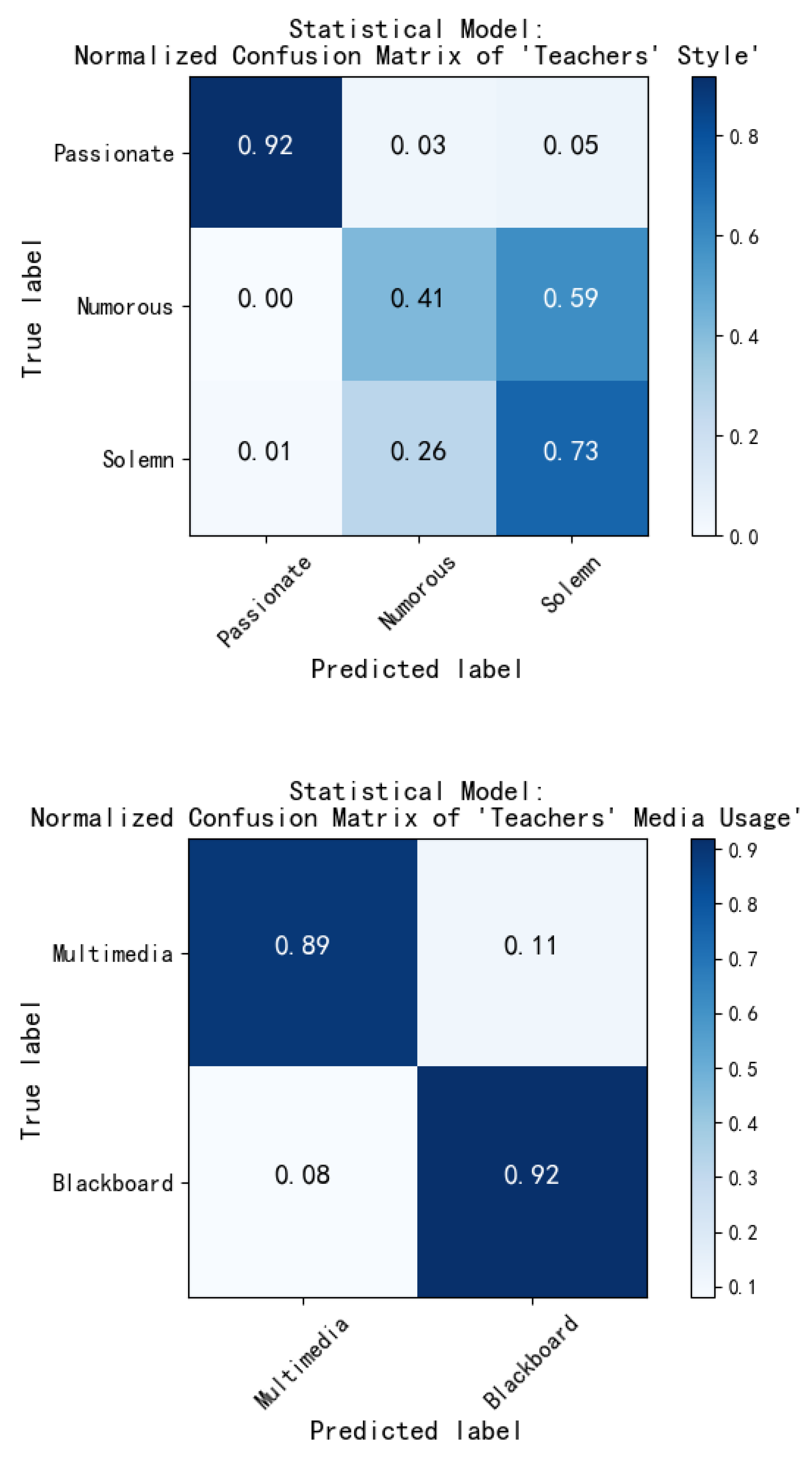
| Teachers’ Style | Passionate | 0.982 | 0.918 | 0.949 | 0.695 | 0.703 | 0.687 | 0.695 | |
| Humorous | 0.511 | 0.414 | 0.457 | ||||||
| Solemn | 0.615 | 0.728 | 0.667 | ||||||
| Teachers’ Media Usage | Multimedia | 0.891 | 0.905 | 0.918 | 0.448 | 0.602 | |||
| Blackboard | 0.919 | ||||||||
| Ensemble Learning | Score Indicator | RMSE |
| Concentration | 8.318 | |
| Participation | 9.375 |
| Ensemble Learning | Category Indicators | Precision | Recall | F1 | Accuracy | M_P | M_R | M_F1 | |
| Teachers’ Type | Indoctrination | 0.947 | 0.935 | 0.941 | 0.785 | 0.755 | 0.761 | 0.758 | |
| Natural | 0.776 | 0.728 | 0.752 | ||||||
| Interactive | 0.542 | 0.619 | 0.619 | ||||||
| Teachers’ Style | Passionate | 0.951 | 0.935 | 0.943 | 0.73 | 0.729 | 0.719 | 0.724 | |
| Humorous | 0.578 | 0.464 | 0.515 | ||||||
| Solemn | 0.66 | 0.756 | 0.705 | ||||||
| Teachers’ Media Usage | Multimedia | 0.881 | 0.89 | 0.897 | 0.433 | 0.584 | |||
| Blackboard | 0.899 | ||||||||
| Statistical Modelling | RMSE | Overall Module Parameters | |||||||
| Concentration | 11.167 | ||||||||
| Participation | 13.409 | Precision | Recall | F1 | Accuracy | M_P | M_R | M_F1 | |
| Teachers’ Type | Indoctrination | 0.987 | 0.938 | 0.962 | 0.815 | 0.789 | 0.791 | 0.790 | |
| Natural | 0.776 | 0.776 | 0.776 | ||||||
| Interactive | 0.604 | 0.659 | 0.630 | ||||||
| Teachers’ Style | Passionate | 0.982 | 0.918 | 0.949 | 0.695 | 0.703 | 0.687 | 0.695 | |
| Humorous | 0.511 | 0.414 | 0.457 | ||||||
| Solemn | 0.615 | 0.728 | 0.667 | ||||||
| Teachers’ Media Usage | Multimedia | 0.891 | 0.905 | 0.918 | 0.448 | 0.602 | |||
| Blackboard | 0.919 | ||||||||
| Ensemble Learning | RMSE | Overall Module Parameters | |||||||
| Concentration | 8.318 | ||||||||
| Participation | 9.375 | Precision | Recall | F1 | Accuracy | M_P | M_R | M_F1 | |
| Teachers’ Type | Indoctrination | 0.947 | 0.935 | 0.941 | 0.785 | 0.755 | 0.761 | 0.758 | |
| Natural | 0.776 | 0.728 | 0.752 | ||||||
| Interactive | 0.542 | 0.619 | 0.619 | ||||||
| Teachers’ Style | Passionate | 0.951 | 0.935 | 0.943 | 0.73 | 0.729 | 0.719 | 0.724 | |
| Humorous | 0.578 | 0.464 | 0.515 | ||||||
| Solemn | 0.66 | 0.756 | 0.705 | ||||||
| Teachers’ Media Usage | Multimedia | 0.881 | 0.89 | 0.897 | 0.433 | 0.584 | |||
| Blackboard | 0.899 | ||||||||
Publisher’s Note: MDPI stays neutral with regard to jurisdictional claims in published maps and institutional affiliations. |
© 2021 by the authors. Licensee MDPI, Basel, Switzerland. This article is an open access article distributed under the terms and conditions of the Creative Commons Attribution (CC BY) license (http://creativecommons.org/licenses/by/4.0/).
Share and Cite
Guo, J.; Bai, L.; Yu, Z.; Zhao, Z.; Wan, B. An AI-Application-Oriented In-Class Teaching Evaluation Model by Using Statistical Modeling and Ensemble Learning. Sensors 2021, 21, 241. https://doi.org/10.3390/s21010241
Guo J, Bai L, Yu Z, Zhao Z, Wan B. An AI-Application-Oriented In-Class Teaching Evaluation Model by Using Statistical Modeling and Ensemble Learning. Sensors. 2021; 21(1):241. https://doi.org/10.3390/s21010241
Chicago/Turabian StyleGuo, Junqi, Ludi Bai, Zehui Yu, Ziyun Zhao, and Boxin Wan. 2021. "An AI-Application-Oriented In-Class Teaching Evaluation Model by Using Statistical Modeling and Ensemble Learning" Sensors 21, no. 1: 241. https://doi.org/10.3390/s21010241