Extended Phase Unwrapping Max-Flow/Min-Cut Algorithm for Multibaseline SAR Interferograms Using a Two-Stage Programming Approach


Abstract
:1. Introduction
2. Review and Analysis of SB PUMA
2.1. Basic Principle of PUMA
2.2. Problem Analysis
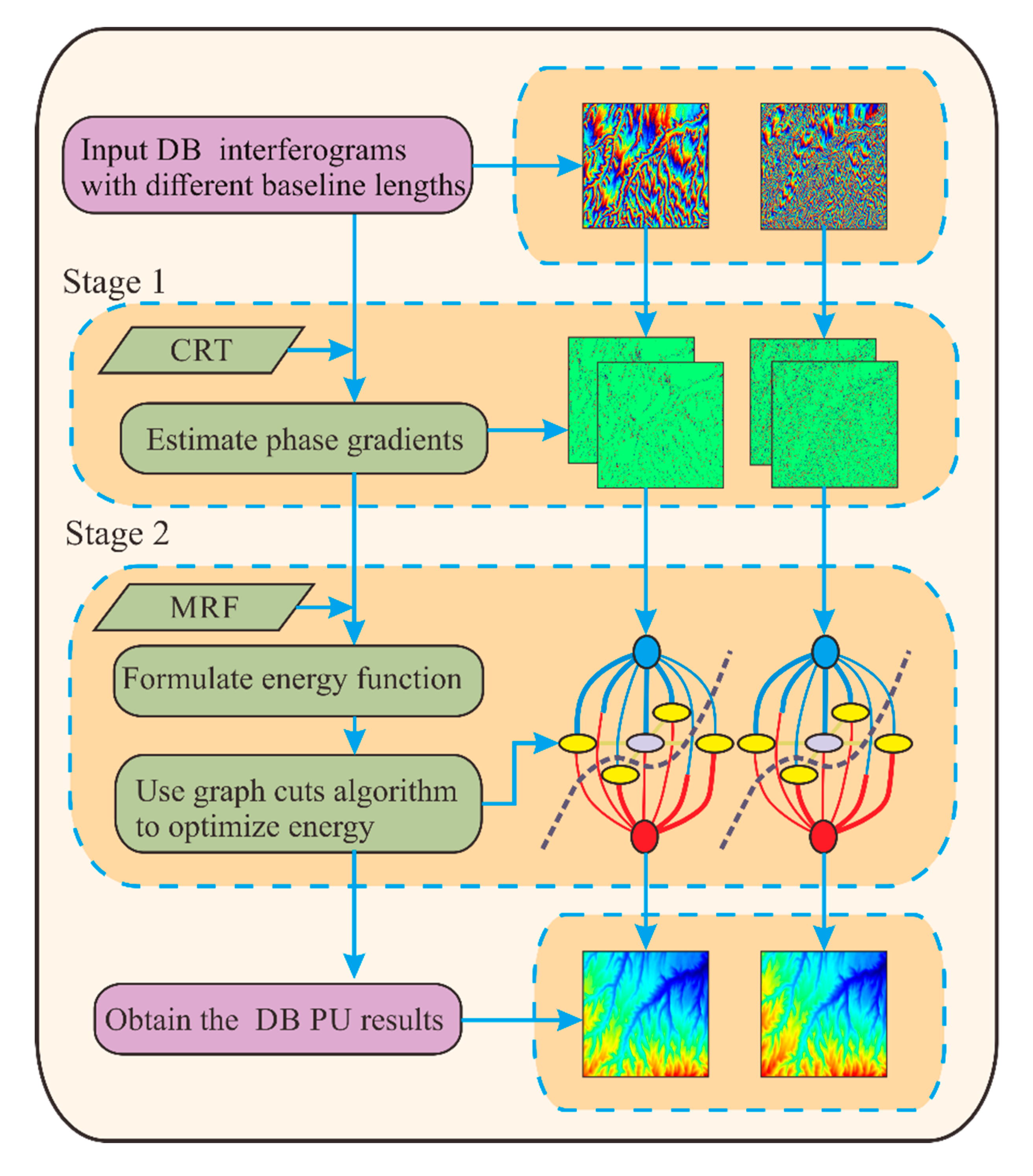
3. TSPA-PUMA Methodfor MB PU
3.1. Stage 1: Estimating the Phase Gradient
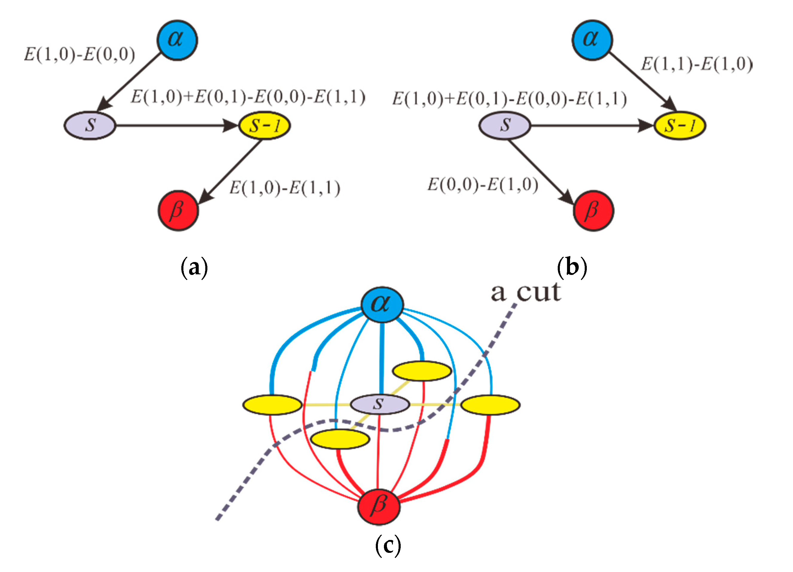
3.2. Stage 2: Unwrapping the Phase Gradient Using Graph Cuts Algorithm
3.3. Analysis of the Noise Robustness
3.4. Analysis of the Time Complexity
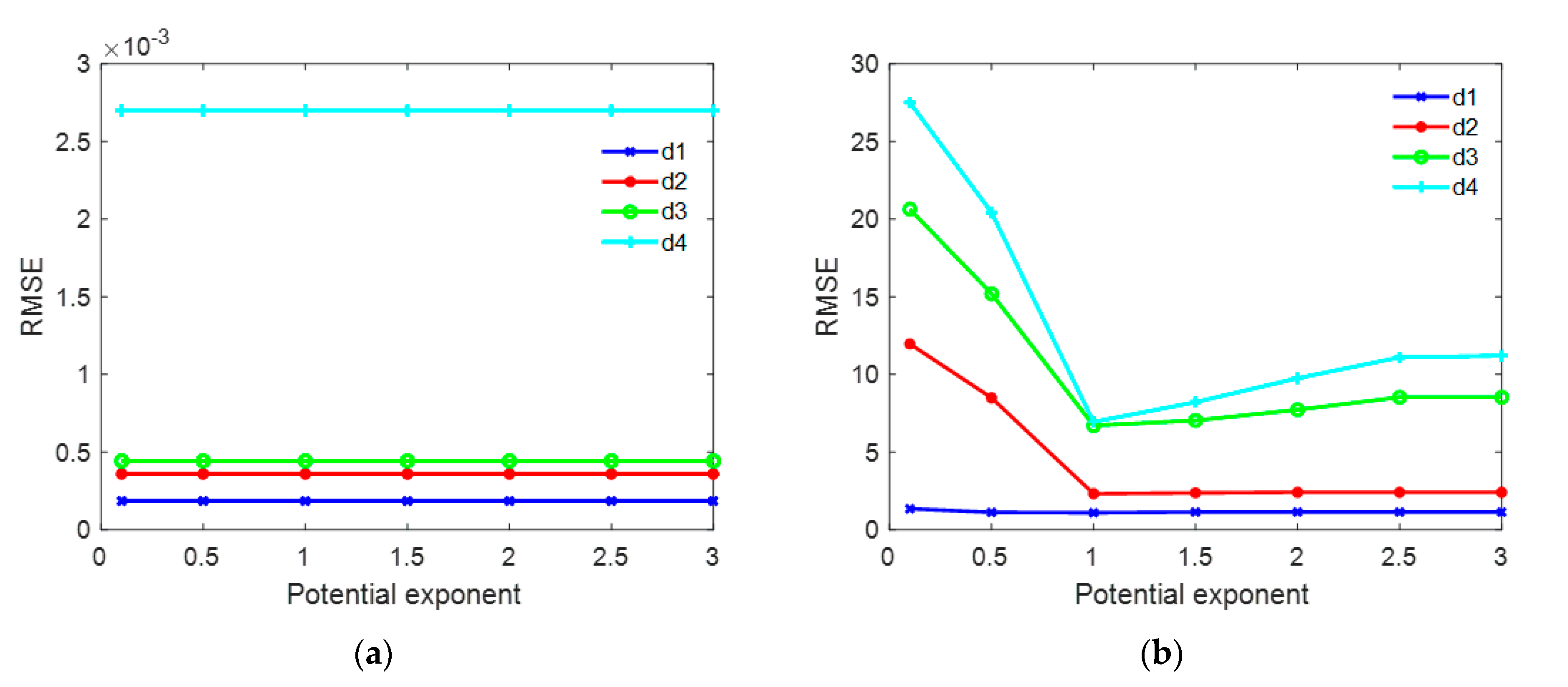
3.5. Analysis of the Parameter Selection
4. Performance Analysis
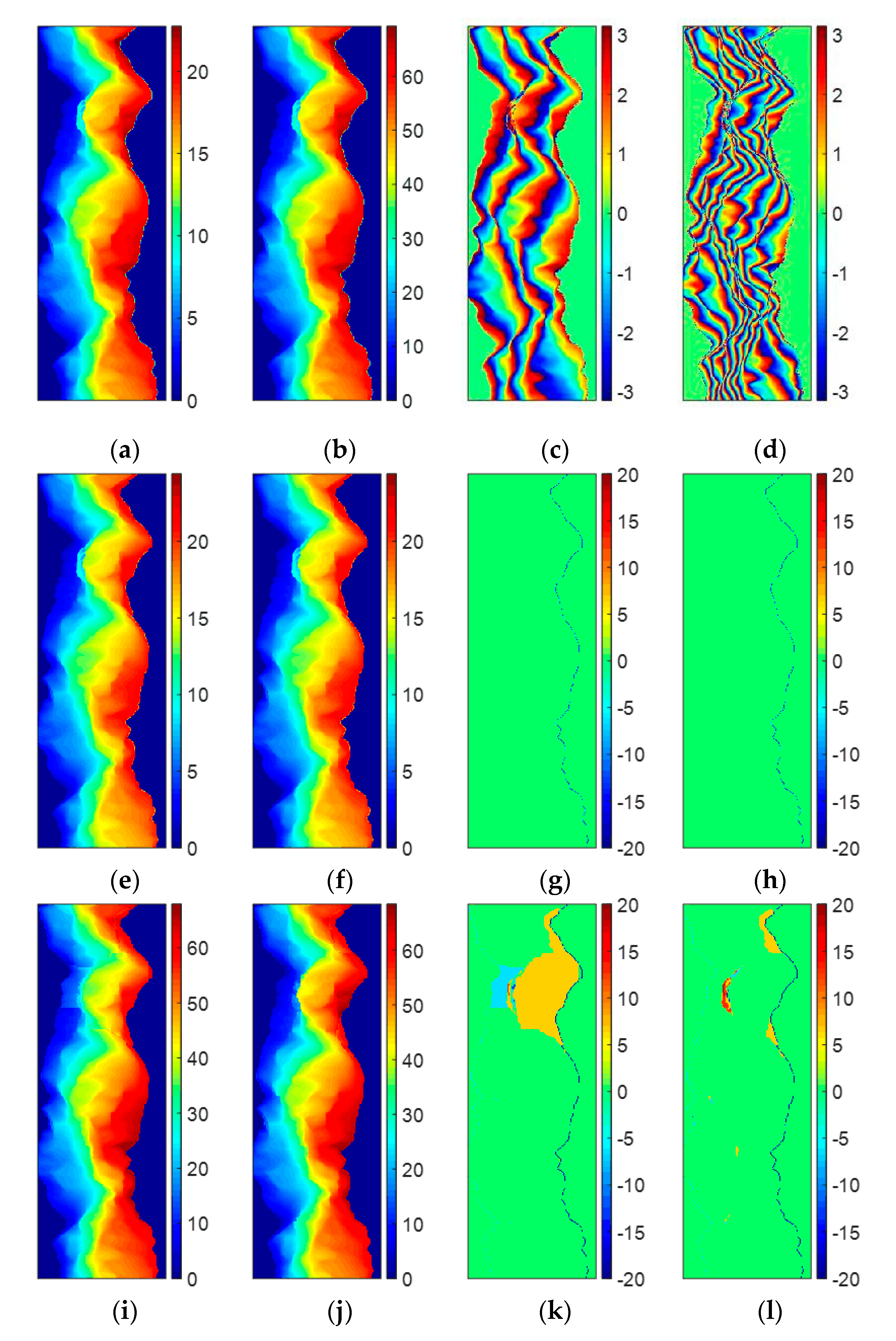
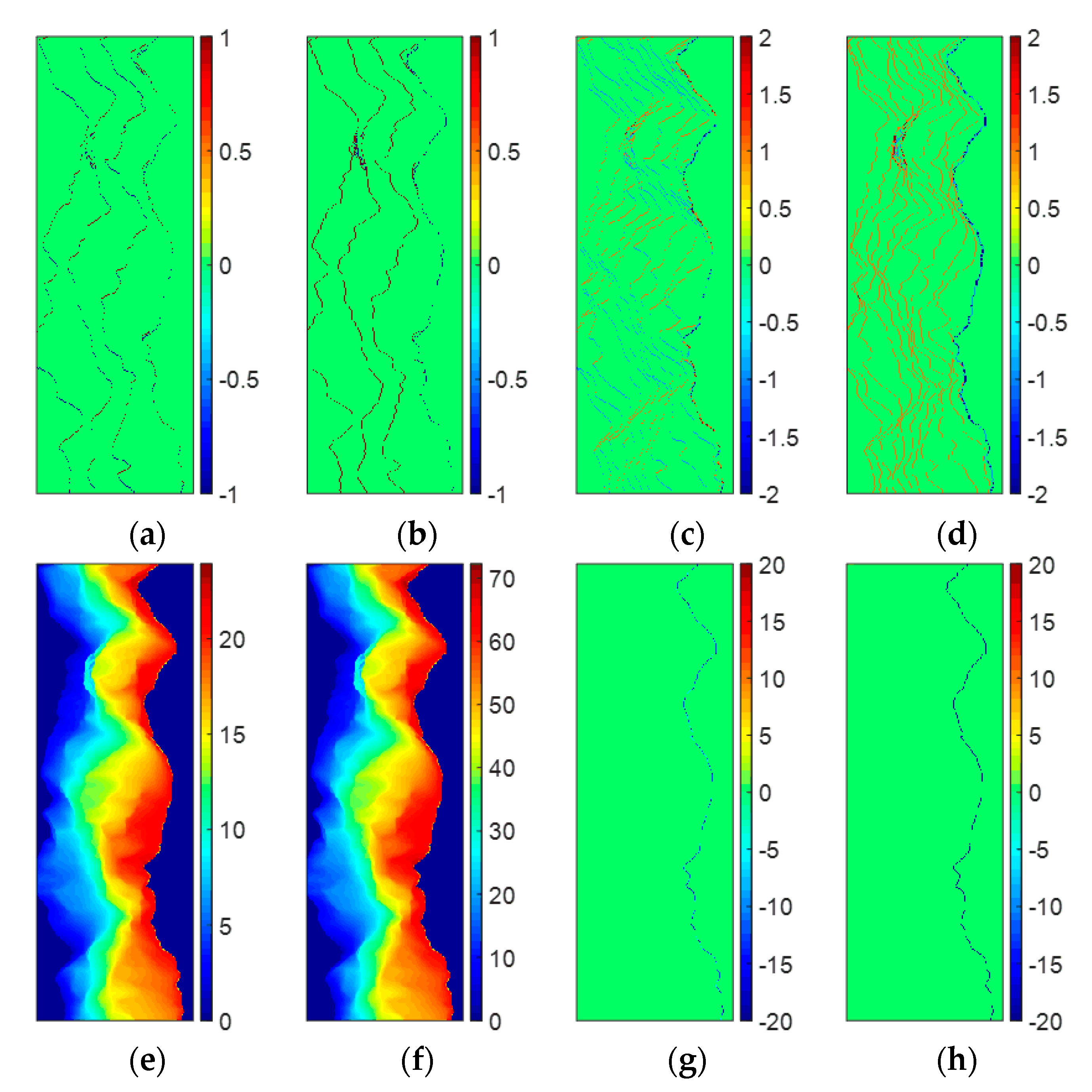
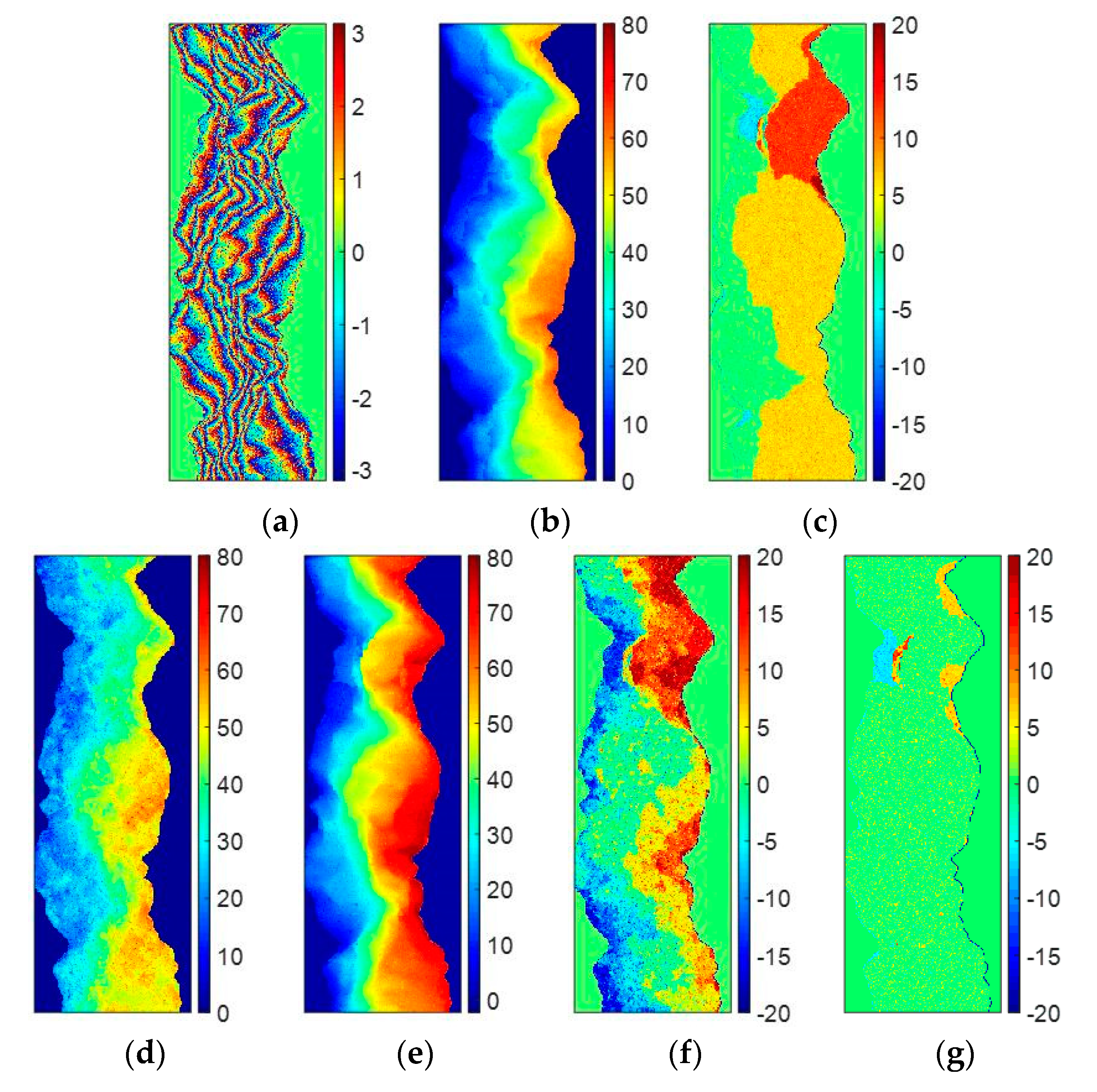
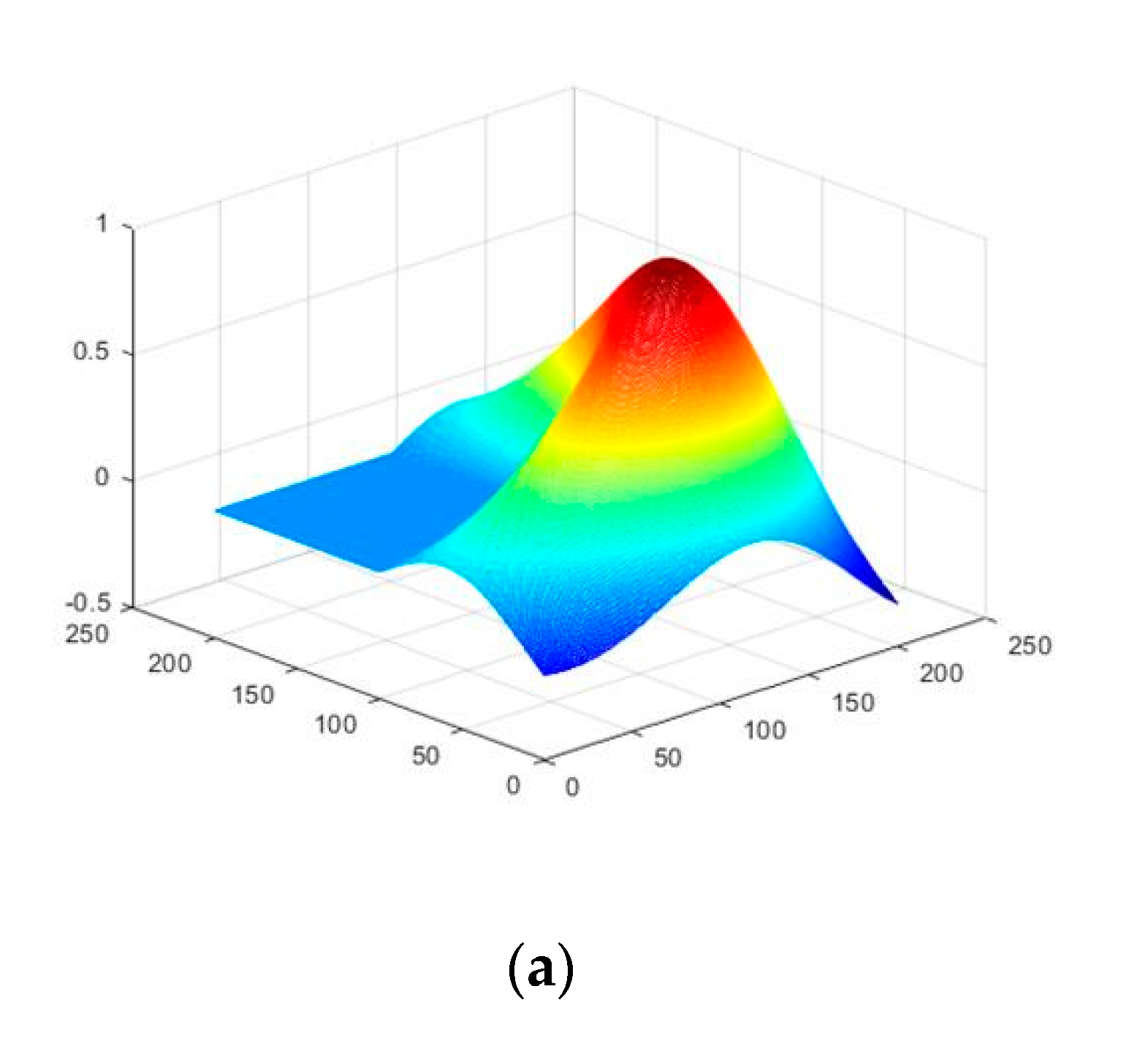
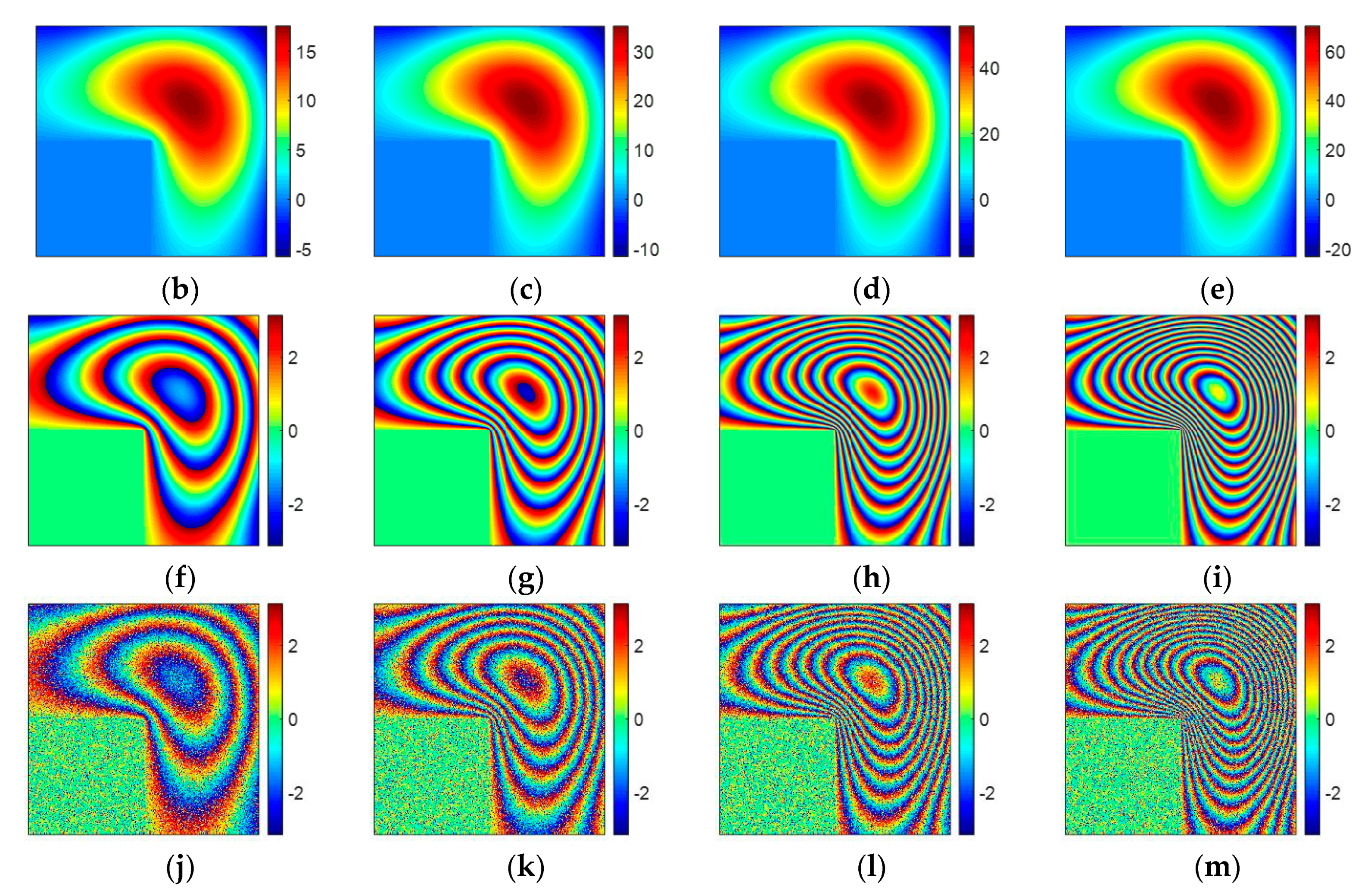
4.1. Experiment 1
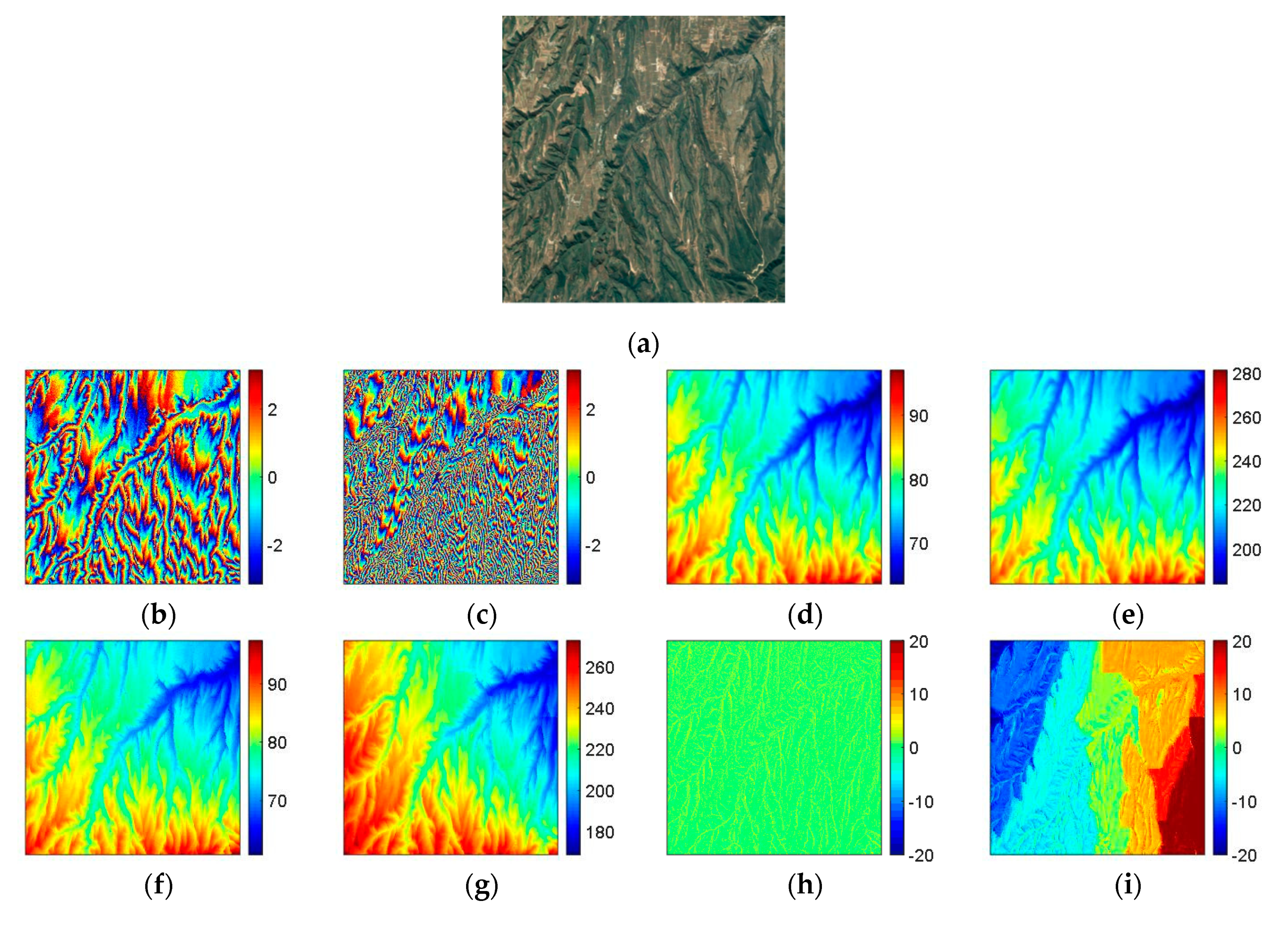
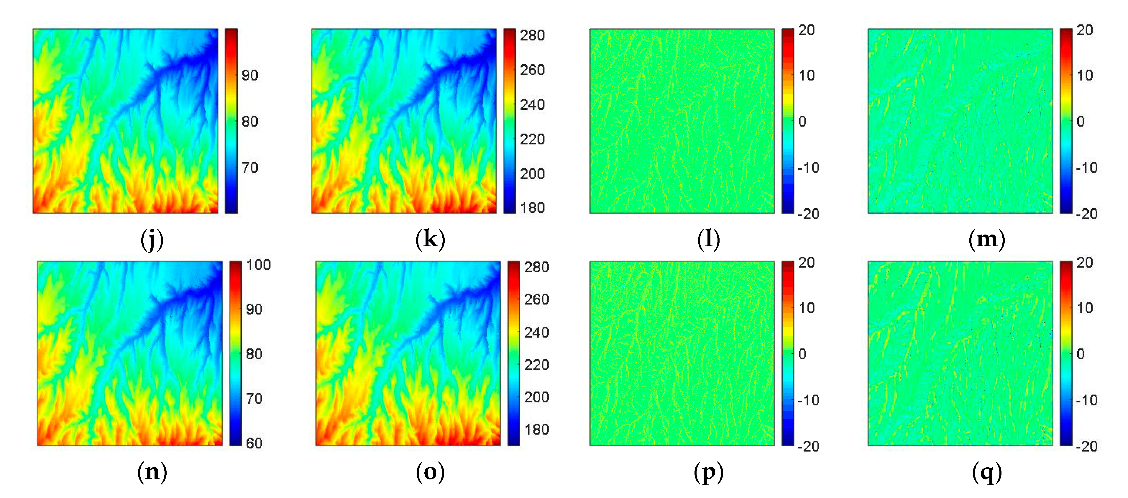
4.2. Experiment 2
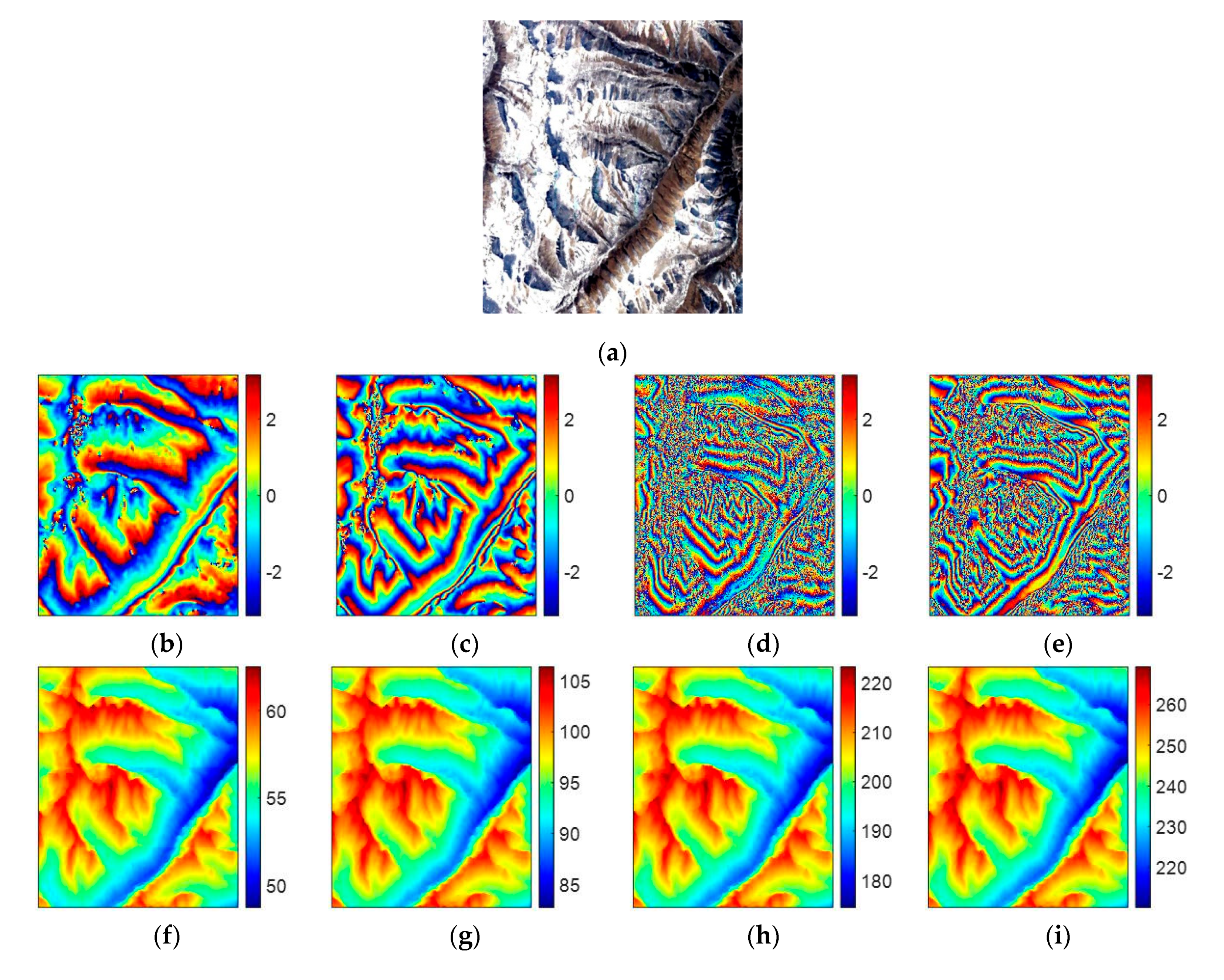
4.3. Experiment 3
4.4. Experiment 4
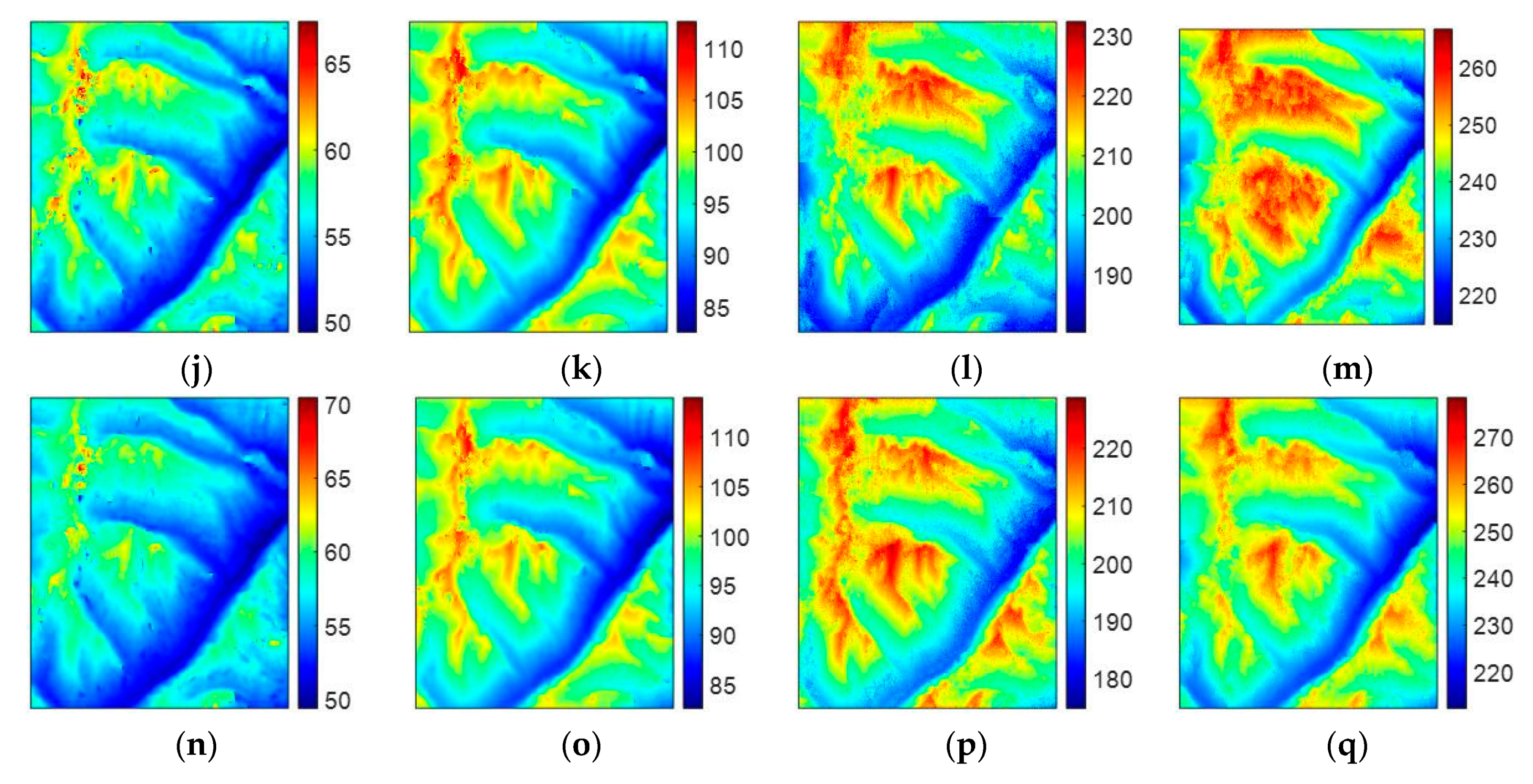
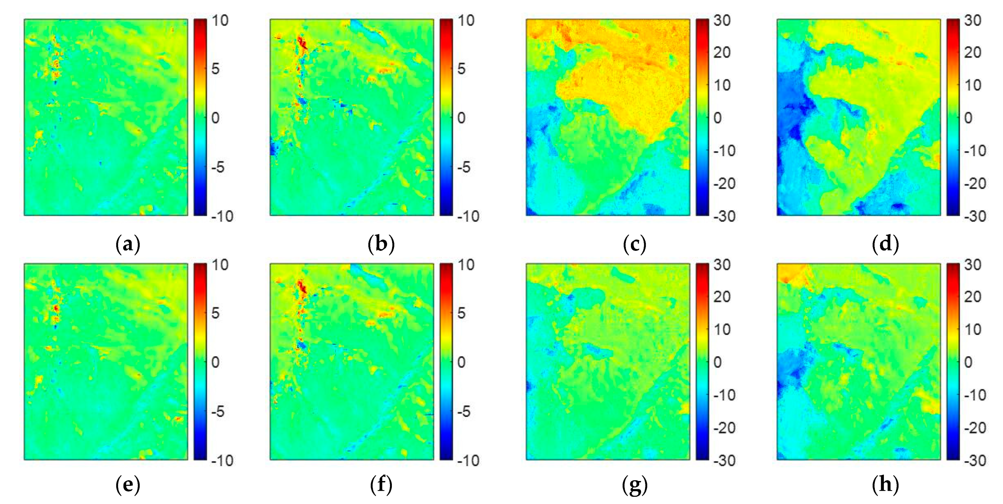
4.5. Experiment 5
5. Conclusions
Author Contributions
Funding
Conflicts of Interest
References
- Moreira, A.; Prats-Iraola, P.; Younis, M.; Krieger, G.; Hajnsek, I.; Papathanassiou, K.P. A tutorial on synthetic aperture radar. IEEE Geosci. Remote Sens. Mag. 2013, 1, 6–43. [Google Scholar] [CrossRef] [Green Version]
- Itoh, K. Analysis of the phase unwrapping problem. Appl. Opt. 1982, 21, 2470. [Google Scholar] [CrossRef] [PubMed]
- Yu, H.; Lan, Y.; Yuan, Z.; Xu, J.; Lee, H. Phase Unwrapping in InSAR: A Review. IEEE Geosci. Remote Sens. Mag. 2019, 7, 40–58. [Google Scholar] [CrossRef]
- Pascazio, V.; Schirinzi, G. Multifrequency InSAR height reconstruction through maximum likelihood estimation of local planes parameters. IEEE Trans. Image Process. 2000, 11, 1478–1489. [Google Scholar] [CrossRef]
- Fornaro, G.; Guarnieri, A.M. Maximum likelihood multi-baseline SAR interferometry. IEEE Proc. Radar Sonar Navig. 2006, 153, 279–288. [Google Scholar] [CrossRef] [Green Version]
- Fornaro, G.; Pauciullo, A.; Sansosti, E. Phase difference-based multichannel phase unwrapping. IEEE Trans. Image Process. 2005, 14, 960–972. [Google Scholar] [CrossRef]
- Ferraiuolo, G.; Pascazio, V.; Schirinzi, G. Maximum a posteriori estimation of height profiles in InSAR imaging. IEEE Geosci. Remote Sens. 2004, 1, 66–70. [Google Scholar] [CrossRef]
- Ferraioli, G.; Shabou, A.; Tupin, F.; Pascazio, V. Multichannel phase unwrapping with graph cuts. IEEE Geosci. Remote Sens. Lett. 2009, 6, 562–566. [Google Scholar] [CrossRef]
- Baselice, F.; Ferraioli, G.; Pascazio, V.; Schirinzi, G. Contextual information-based multichannel synthetic aperture radar interferometry: Addressing DEM reconstruction using contextual information. IEEE Signal Process. Mag. 2014, 31, 59–68. [Google Scholar] [CrossRef]
- Ferraiuolo, G.; Meglio, F.; Pascazio, V.; Schirinzi, G. DEM reconstruction accuracy in multichannel SAR interferometry. IEEE Trans. Geosci. Remote Sens. 2009, 47, 191–201. [Google Scholar] [CrossRef]
- Yu, H.; Li, Z.; Bao, Z. A cluster-analysis-based efficient multibaseline phase-unwrapping algorithm. IEEE Trans. Geosci. Remote Sens. 2011, 49, 478–487. [Google Scholar] [CrossRef]
- Liu, H.; Xing, M.; Bao, Z. A cluster-analysis-based noise-robust phase-unwrapping algorithm for multibaseline interferograms. IEEE Trans. Geosci. Remote Sens. 2015, 53, 494–504. [Google Scholar]
- Jiang, Z.; Wang, J.; Song, Q.; Zhou, Z. A refined cluster-analysis-based multibaseline phase-unwrapping algorithm. IEEE Geosci. Remote Sens. Lett. 2017, 14, 1565–1569. [Google Scholar] [CrossRef]
- Liu, H.; Xing, M.; Bao, Z. A novel mixed-norm multibaseline phase-unwrapping algorithm based on linear programming. IEEE Geosci. Remote Sens. Lett. 2015, 12, 1086–1090. [Google Scholar] [CrossRef]
- Yuan, Z.; Deng, Y.; Li, F.; Wang, R.; Liu, G.; Han, X. Multichannel InSAR DEM reconstruction through improved closed-form robust Chinese remainder theorem. IEEE Geosci. Remote Sens. Lett. 2013, 10, 1314–1318. [Google Scholar] [CrossRef]
- Jin, B.; Guo, J.; Wei, P.; Su, B.; He, D. Multi-baseline InSAR phase unwrapping method based on mixed-integer optimisation model. IET Radar Sonar Navig. 2018, 12, 694–701. [Google Scholar] [CrossRef]
- Kim, M.G.; Griffiths, H.D. Phase unwrapping of multibaseline interferometry using Kalman filtering. In Proceedings of the 7th International Conference on Image Processing and its Applications, London, UK, 13–15 July 1999; pp. 251–253. [Google Scholar]
- Ferretti, A.; Prati, C.; Rocca, R. Multibaseline InSAR DEM recon-struction: The wavelet approach. IEEE Trans. Geosci. Remote Sens. 1999, 37, 705–715. [Google Scholar] [CrossRef]
- Yu, H.; Lan, Y. Robust two-dimensional phase unwrapping for multibaseline sar interferograms: A two-stage programming approach. IEEE Trans. Geosci. Remote Sens. 2016, 54, 5217–5225. [Google Scholar] [CrossRef]
- Costantini, M. A novel phase unwrapping method based on network programming. IEEE Trans. Geosci. Remote Sens. 1998, 36, 813–821. [Google Scholar] [CrossRef]
- Ahuja, R.; Magnanti, T.; Orlin, J. Network Flows: Theory, Algorithms and Applications; Prentice Hall: Upper Saddle River, NJ, USA, 1993; ISBN-13 978-0136175490. [Google Scholar]
- Yu, H.; Xing, M.; Bao, Z. A fast phase unwrapping method for largescale interferograms. IEEE Trans. Geosci. Remote Sens. 2013, 51, 4240–4248. [Google Scholar]
- Yu, H.; Lan, Y.; Xu, J.; An, D.; Lee, H. Large-scale L0-norm and L1-norm two-dimensional phase unwrapping. IEEE Trans. Geosci. Remote Sens. 2017, 55, 4712–4728. [Google Scholar] [CrossRef]
- Lan, Y.; Yu, H.; Xing, M. Refined Two-Stage Programming-Based Multi-Baseline Phase Unwrapping Approach Using Local Plane Model. Remote Sens. 2019, 11, 491. [Google Scholar] [CrossRef] [Green Version]
- Gao, Y.; Zhang, S.; Li, T.; Chen, Q.; Zhang, X.; Li, S. Refined Two-Stage Programming Approach of Phase Unwrapping for Multi-Baseline SAR Interferograms Using the Unscented Kalman Filter. Remote Sens. 2019, 11, 199. [Google Scholar] [CrossRef] [Green Version]
- Yu, H.; Zhou, Y.; Ivey, S.; Lan, Y. Large-scale multibaseline phase unwrapping: Interferogram segmentation based on multibaseline envelope-sparsity theorem. IEEE Trans. Geosci. Remote Sens. 2019, 57, 9308–9322. [Google Scholar] [CrossRef]
- Bioucas-Dias, J.; Valadao, G. Phase unwrapping via graph cuts. IEEE Trans. Image Process 2007, 16, 698–709. [Google Scholar] [CrossRef] [PubMed]
- Zhou, L.; Chai, D.; Xia, Y.; Xie, C. An extended PUMA algorithm for multibaseline InSAR DEM reconstruction. Int. J. Remote Sens. 2019, 40, 7830–7851. [Google Scholar] [CrossRef]
- Liu, G.; Wang, R.; Deng, Y.; Chen, R.; Shao, Y.; Yuan, Z. A new quality map for 2-D phase unwrapping based on gray level cooccurrence matrix. IEEE Geosci. Remote Sens. Lett. 2014, 11, 444–448. [Google Scholar] [CrossRef]
- Kolmogorov, V.; Zabih, R. What energy functions can be minimized via graph cuts? IEEE Trans. Pattern Anal. Mach. Intell. 2004, 26, 147–159. [Google Scholar] [CrossRef] [Green Version]
- Ghiglia, D.C.; Pritt, M.D. Two-Dimensional Phase Unwrapping: Theory, Algorithms, and Software; Wiley-Interscience: New York, NY, USA, 1998; ISBN 0-471-24935-1. [Google Scholar]
- Colesanti, C.; Ferretti, A.; Prati, C.; Rocca, F. Monitoring landslides and tectonic motions with the permanent scatterers technique. Eng. Geol. 2003, 68, 3–14. [Google Scholar] [CrossRef]
- Vineet, V.; Narayanan, P.J. CUDA cuts: Fast graph cuts on the GPU. In Proceedings of the 2008 IEEE Computer Society Conference on Computer Vision and Pattern Recognition Workshops, Anchorage, AK, USA, 23–28 June 2008; pp. 1–8. [Google Scholar]
- Bioucas-Dias, J.; Valadão, G. PUMA Algorithm (Phase Unwrapping, Via Graph Cuts) (MATLAB Code). 2007. Available online: http://www.lx.it.pt/~bioucas/code.htm. (accessed on 10 November 2019).
- Lan, Y.; Yu, H. TSPA Multi-Baseline Phase Unwrapping Method (MATLAB Code). 2018. Available online: http://rscl-grss.org/codelibrary/43c468514e6bb1c32994a2f9dbfc5be2.zip (accessed on 10 November 2018).
- Lee, J.-S.; Hoppel, K.W.; Mango, S.A.; Miller, A.R. Intensity and phase statistics of multilook polarimetric and interferometric SAR imagery. IEEE Trans. Geosci. Remote Sens. 1994, 32, 1017–1028. [Google Scholar]
- Yu, H.; Lee, H.; Cao, N.; Lan, Y. Optimal Baseline Design for Multibaseline InSAR Phase Unwrapping. IEEE Trans. Geosci. Remote Sens. 2019, 57, 5738–5750. [Google Scholar] [CrossRef]


| Orbit Altitude | Incidence Angle | Wavelength |
| 6885 km | 46° | 0.031 m |
| Interferogram | Baseline Length | |
| Figure 1c | 150 m | |
| Figure 1d | 330 m | |
| U Method | Short Baseline | Long Baseline | ||
|---|---|---|---|---|
| Figure | RMSE | Figure | RMSE | |
| PUMA with potential exponent 1 | Figure 1g | 0.9505 | Figure 1k | 3.6438 |
| PUMA with potential exponent 0.5 | Figure 1h | 0.9505 | Figure 1l | 3.2356 |
| TSPA-PUMA | Figure 4g | 0.9164 | Figure 4h | 0.9164 |
| ID | Number of Interferograms | Baseline Length (m) | RMSE | |||||||
|---|---|---|---|---|---|---|---|---|---|---|
| 1 | 2 | 150 | 330 | 7.6592 | ||||||
| 2 | 3 | 70 | 150 | 330 | 6.9732 | |||||
| 3 | 4 | 70 | 150 | 330 | 471 | 6.7486 | ||||
| 4 | 5 | 70 | 150 | 330 | 471 | 550 | 6.6240 | |||
| 5 | 6 | 70 | 150 | 330 | 471 | 550 | 631 | 4.6023 | ||
| 6 | 7 | 70 | 150 | 330 | 471 | 550 | 631 | 753 | 4.3318 | |
| 7 | 8 | 70 | 150 | 330 | 471 | 550 | 631 | 753 | 831 | 3.4297 |
| Orbit Altitude | Incidence Angle | Wavelength | Latitude | longitude |
|---|---|---|---|---|
| 514.8 km | 36.6° | 0.032 m | 35.82° | 109.28° |
| Interferogram | Figure 6b | Figure 6c | ||
| Date of Master Channel | 2 April 2014 | 21 October 2012 | ||
| Date of Slave Channel | 2 April 2014 | 21 October 2012 | ||
| Baseline Length | 130.62 m | 370.45 m | ||
| Resolution | Range (Vertical) | 5.46 m | Azimuth (Horizontal) | 8.15 m |
| Image Size | Range | 1000 pixels | Azimuth | 1000 pixels |
| PU Method | Short Baseline | Long Baseline | ||||
|---|---|---|---|---|---|---|
| Figure | RMSE | Time (s) | Figure | RMSE | Time (s) | |
| PUMA with potential exponent 0.5 | Figure 6h | 0.6871 | 116.18 | Figure 6i | 10.0892 | 303.83 |
| TSPA | Figure 6l | 0.6114 | 665.92 | Figure 6m | 1.91 | 1941.04 |
| TSPA-PUMA | Figure 6p | 0.69 | 65.81 | Figure 6q | 1.7616 | 231.72 |
| Orbit Altitude | Incidence Angle | Wavelength | Latitude | longitude |
|---|---|---|---|---|
| 698.51 km | 38.75° | 0.236m | 30.91° | 94.23° |
| Interferogram | Figure 7b | Figure 7c | Figure 7d | Figure 7e |
| Date of Master Channel | 18 August 2007 | 18 August 2007 | 18 August 2007 | 18 August 2007 |
| Date of Slave Channel | 3 October 2007 | 3 July 2007 | 3 January 2008 | 8 October 2009 |
| Baseline Length | 113.36 m | 193.15 m | 406.00 m | 440.68 m |
| Resolution | Range (Vertical) | 9.37 m | Azimuth (Horizontal) | 19.00 m |
| Image Size | Range | 601 pixels | Azimuth | 501 pixels |
| PU Method | Interferogram 1 | Interferogram 2 | Interferogram 3 | Interferogram 4 | ||||
|---|---|---|---|---|---|---|---|---|
| Figure | RMSE | Figure | RMSE | Figure | RMSE | Figure | RMSE | |
| PUMA with potential exponent 0.5 | Figure 8a | 0.8719 | Figure 8b | 1.1576 | Figure 8c | 7.4004 | Figure 8d | 7.4951 |
| TSPA-PUMA | Figure 8e | 0.8577 | Figure 8f | 1.0860 | Figure 8g | 3.4688 | Figure 8h | 4.6751 |
© 2020 by the authors. Licensee MDPI, Basel, Switzerland. This article is an open access article distributed under the terms and conditions of the Creative Commons Attribution (CC BY) license (http://creativecommons.org/licenses/by/4.0/).
Share and Cite
Zhou, L.; Lan, Y.; Xia, Y.; Gong, S. Extended Phase Unwrapping Max-Flow/Min-Cut Algorithm for Multibaseline SAR Interferograms Using a Two-Stage Programming Approach. Sensors 2020, 20, 375. https://doi.org/10.3390/s20020375
Zhou L, Lan Y, Xia Y, Gong S. Extended Phase Unwrapping Max-Flow/Min-Cut Algorithm for Multibaseline SAR Interferograms Using a Two-Stage Programming Approach. Sensors. 2020; 20(2):375. https://doi.org/10.3390/s20020375
Chicago/Turabian StyleZhou, Lifan, Yang Lan, Yu Xia, and Shengrong Gong. 2020. "Extended Phase Unwrapping Max-Flow/Min-Cut Algorithm for Multibaseline SAR Interferograms Using a Two-Stage Programming Approach" Sensors 20, no. 2: 375. https://doi.org/10.3390/s20020375