Accuracy–Power Controllable LiDAR Sensor System with 3D Object Recognition for Autonomous Vehicle


Abstract
:1. Introduction
2. Related Works
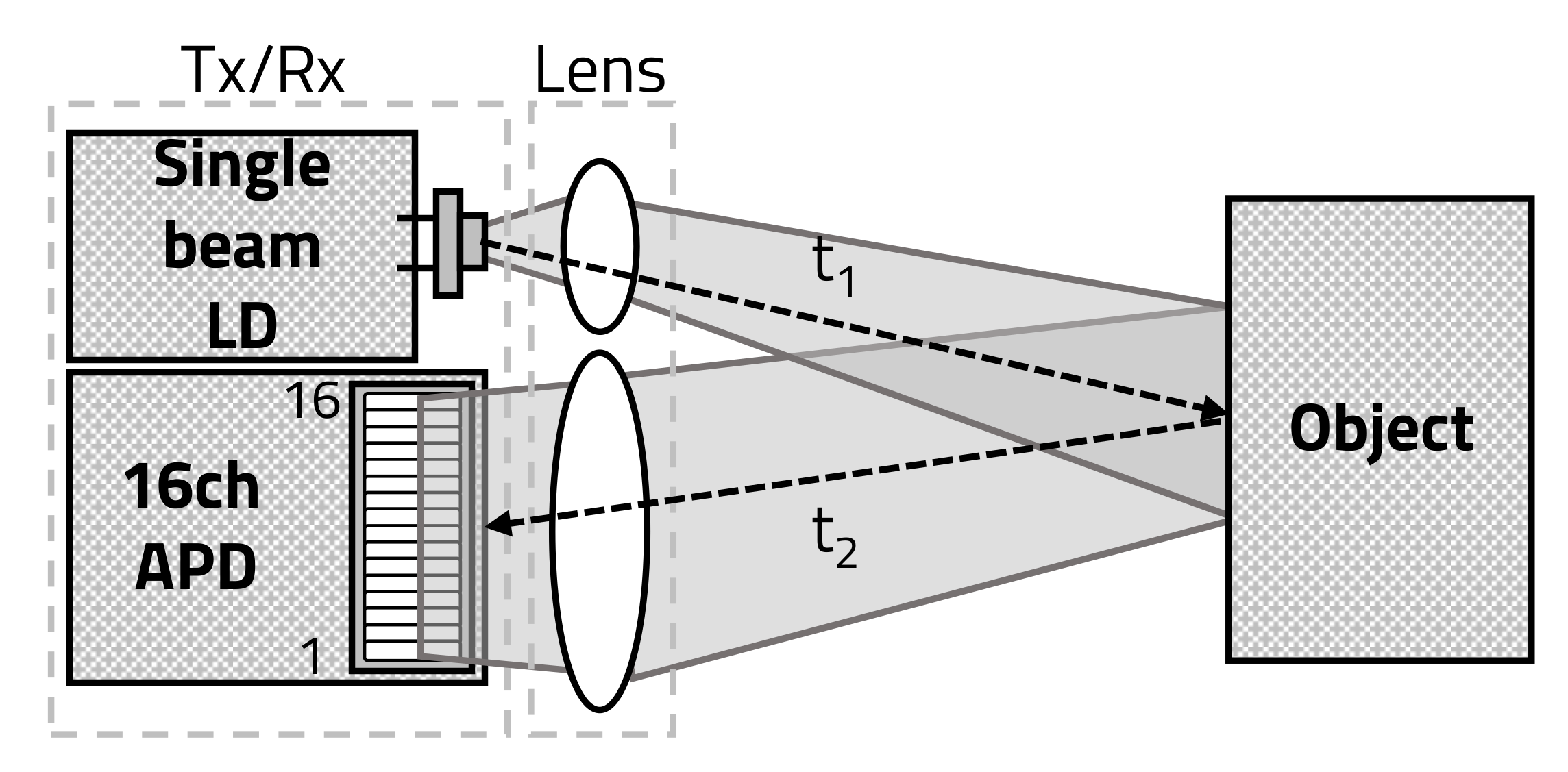
3. Characteristics of Multi-Channel Scanning LiDAR Sensors
3.1. Conventional Multi-Channel Scanning LiDAR Sensors
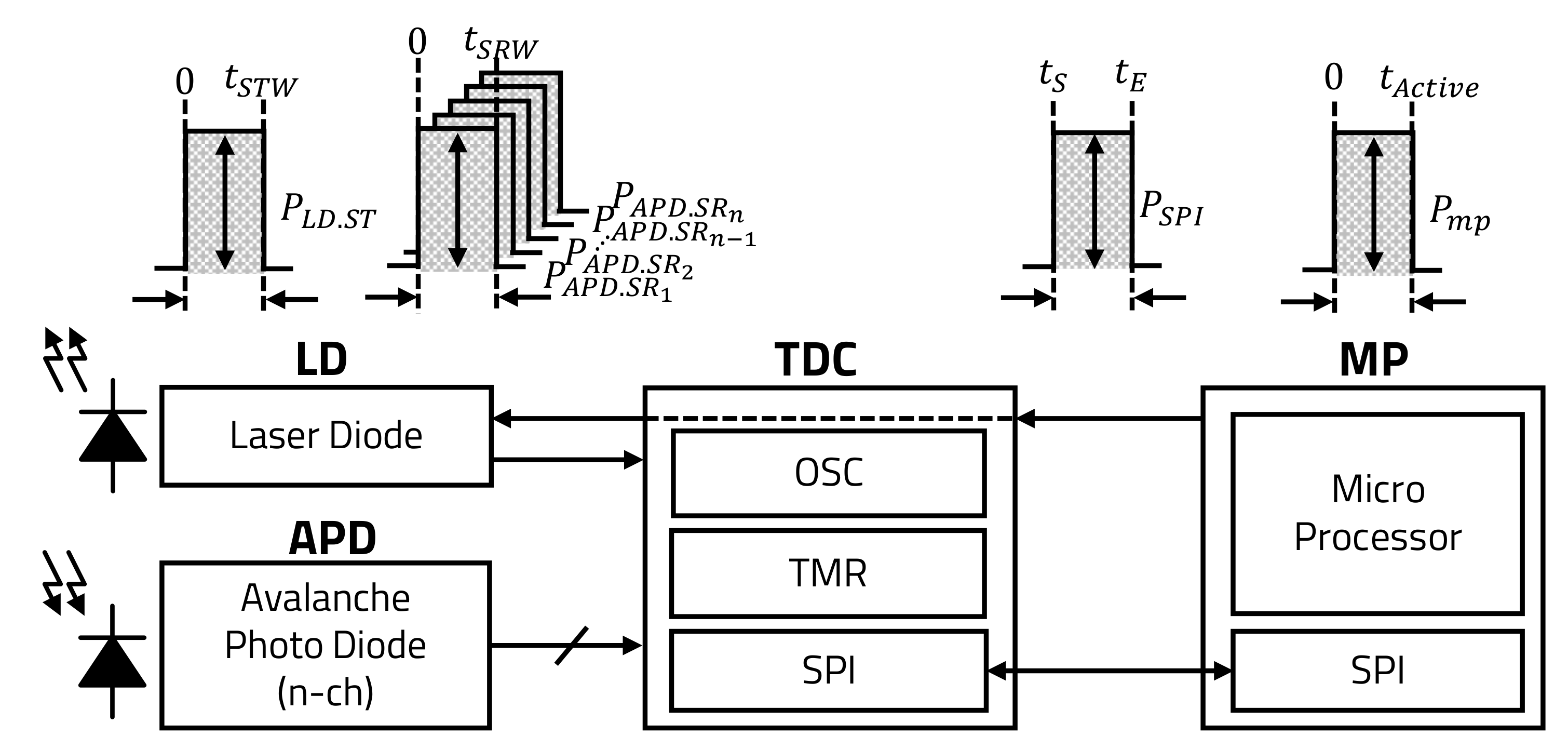
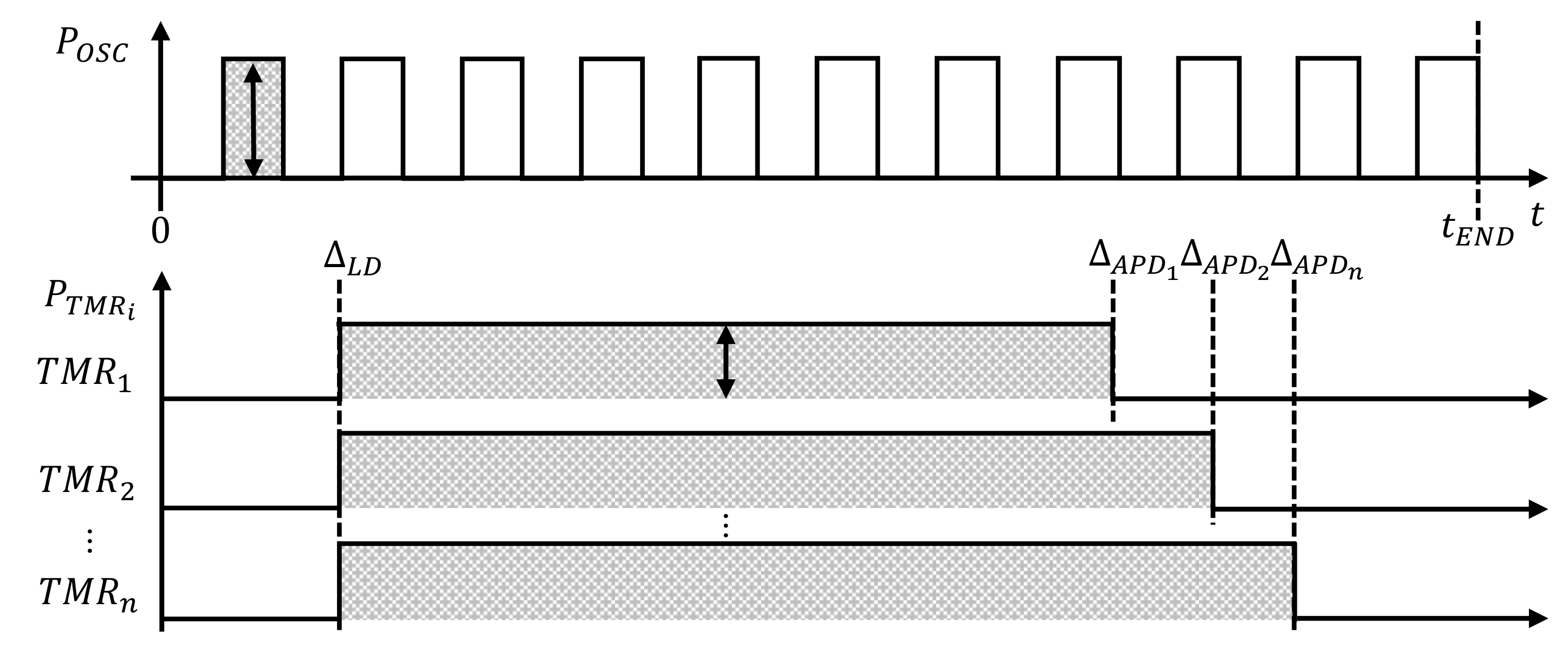
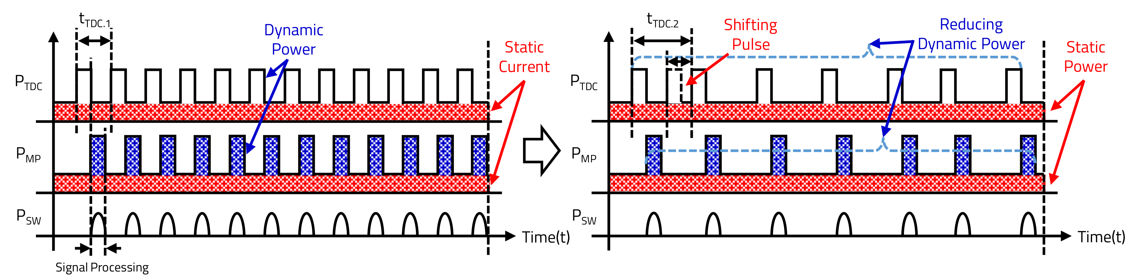
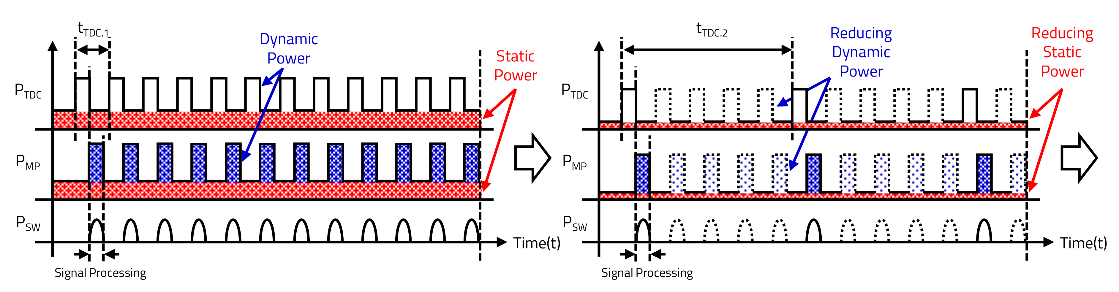
3.1.1. Time-Domain of TDC Operations
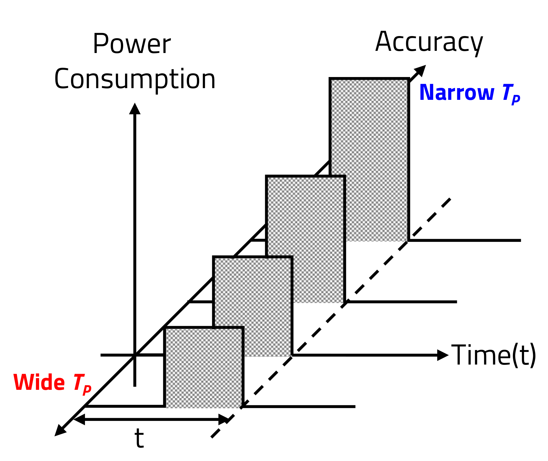
3.1.2. Power Consumption of LiDAR Sensor
3.2. Proposed LiDAR Sensor
3.2.1. Speed Detection-Based LiDAR Sensor Control
| Algorithm 1: Speed detection-based accuracy control. |
 |
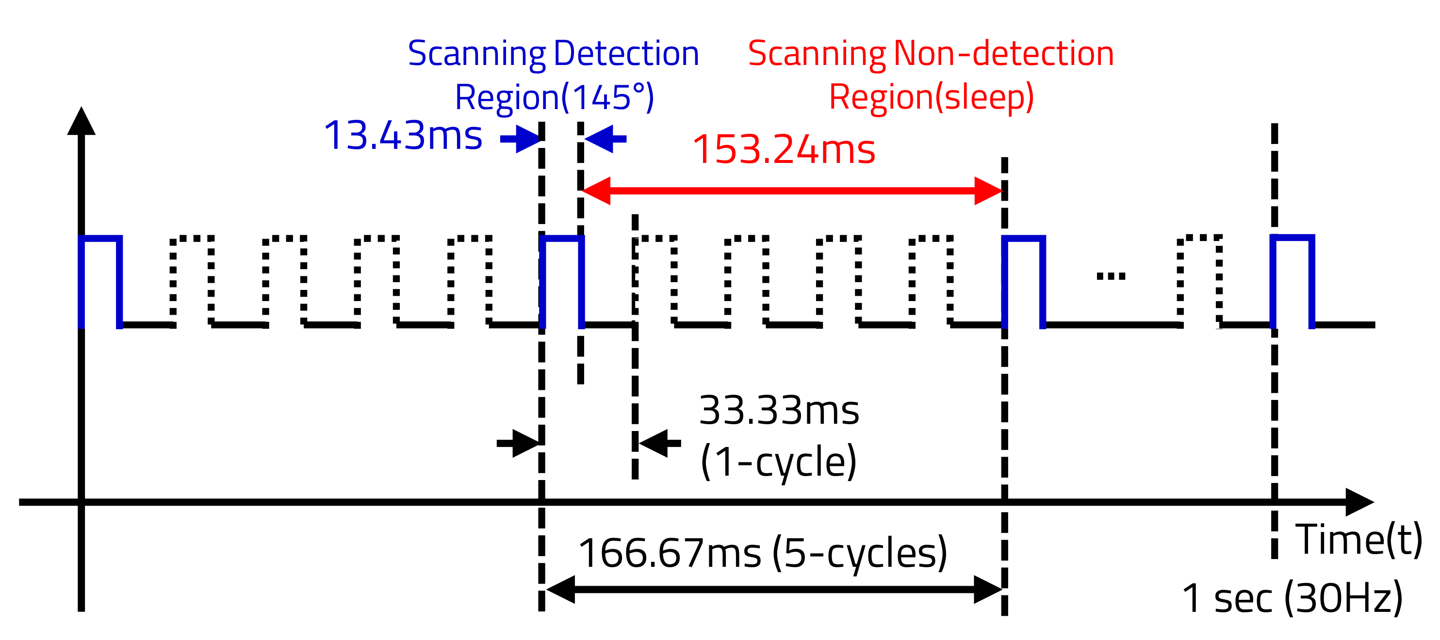
3.2.2. Environment Sensing-Based LiDAR Sensor Control
| Algorithm 2: Environment sensing-based accuracy control. |
 |
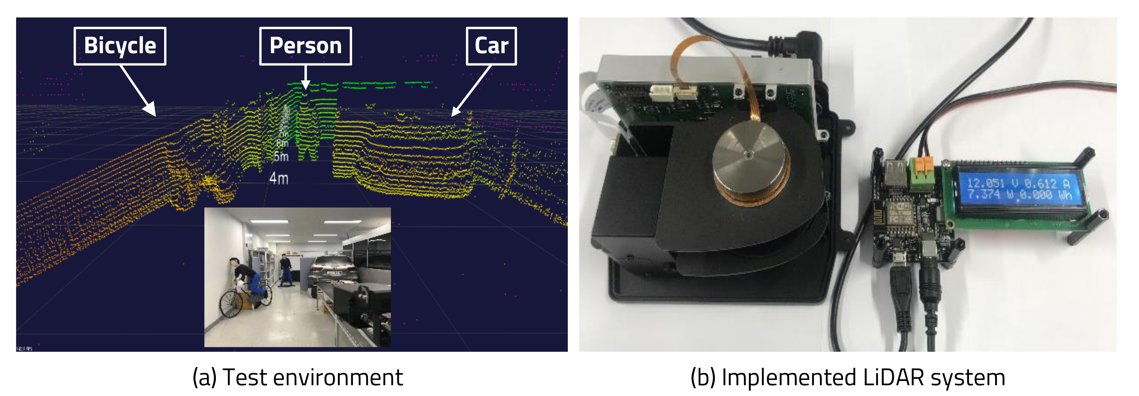
4. Implementation and Experiment
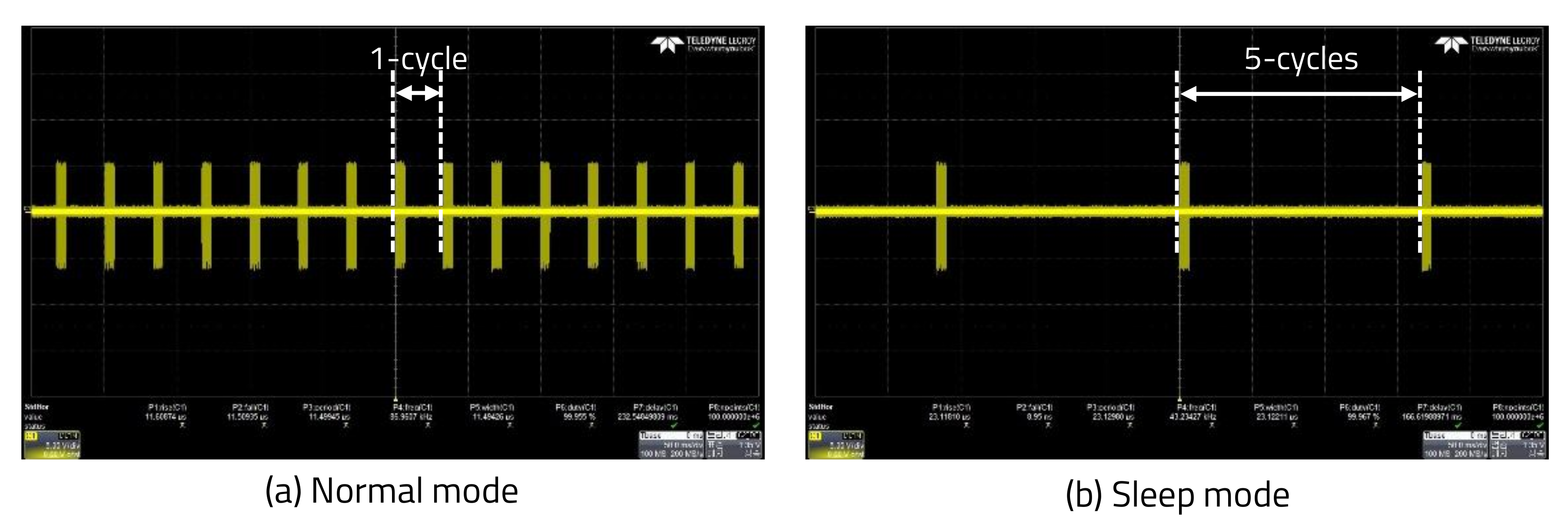
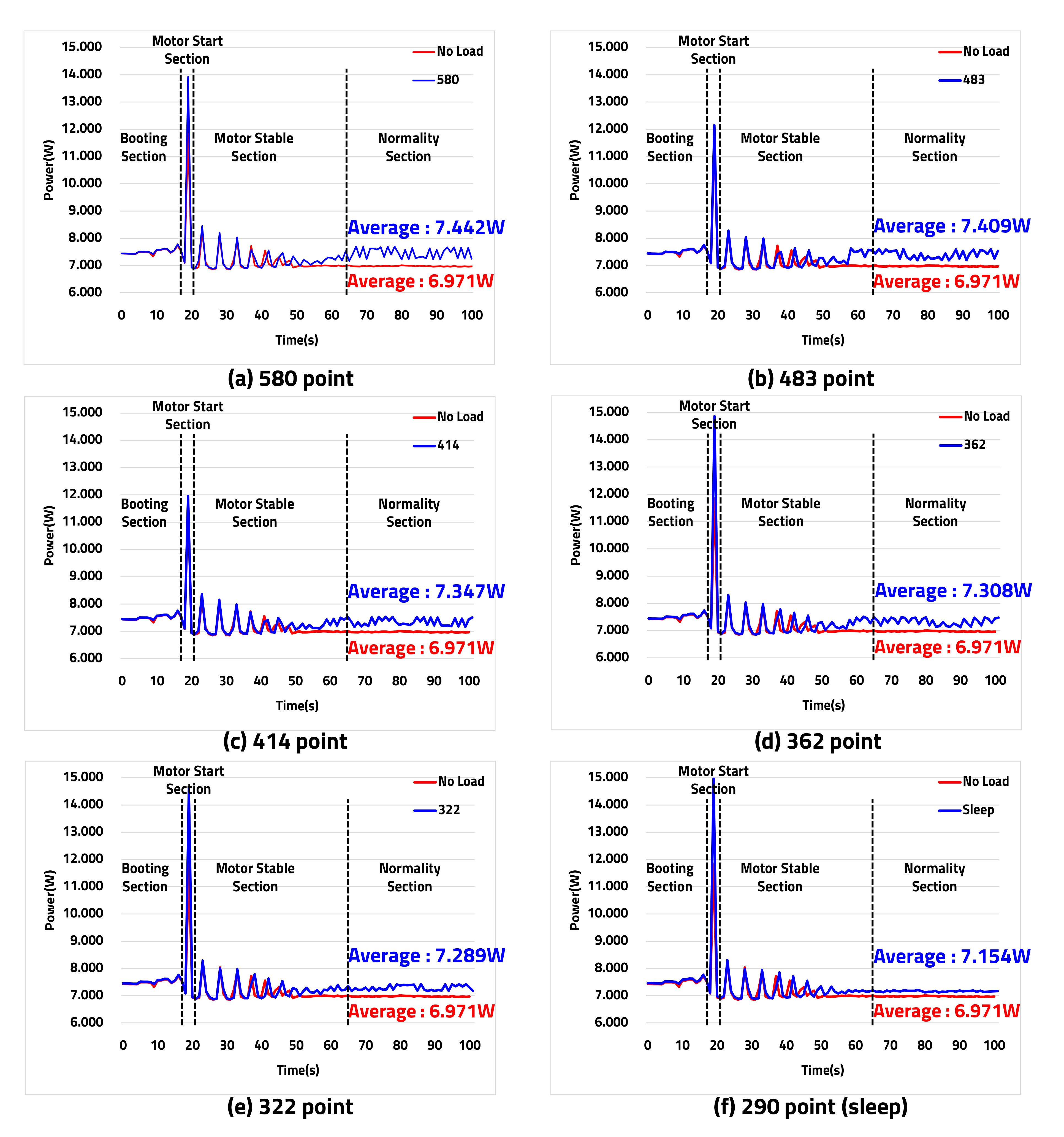
4.1. Power-Consumption Measurement of LiDAR Sensor
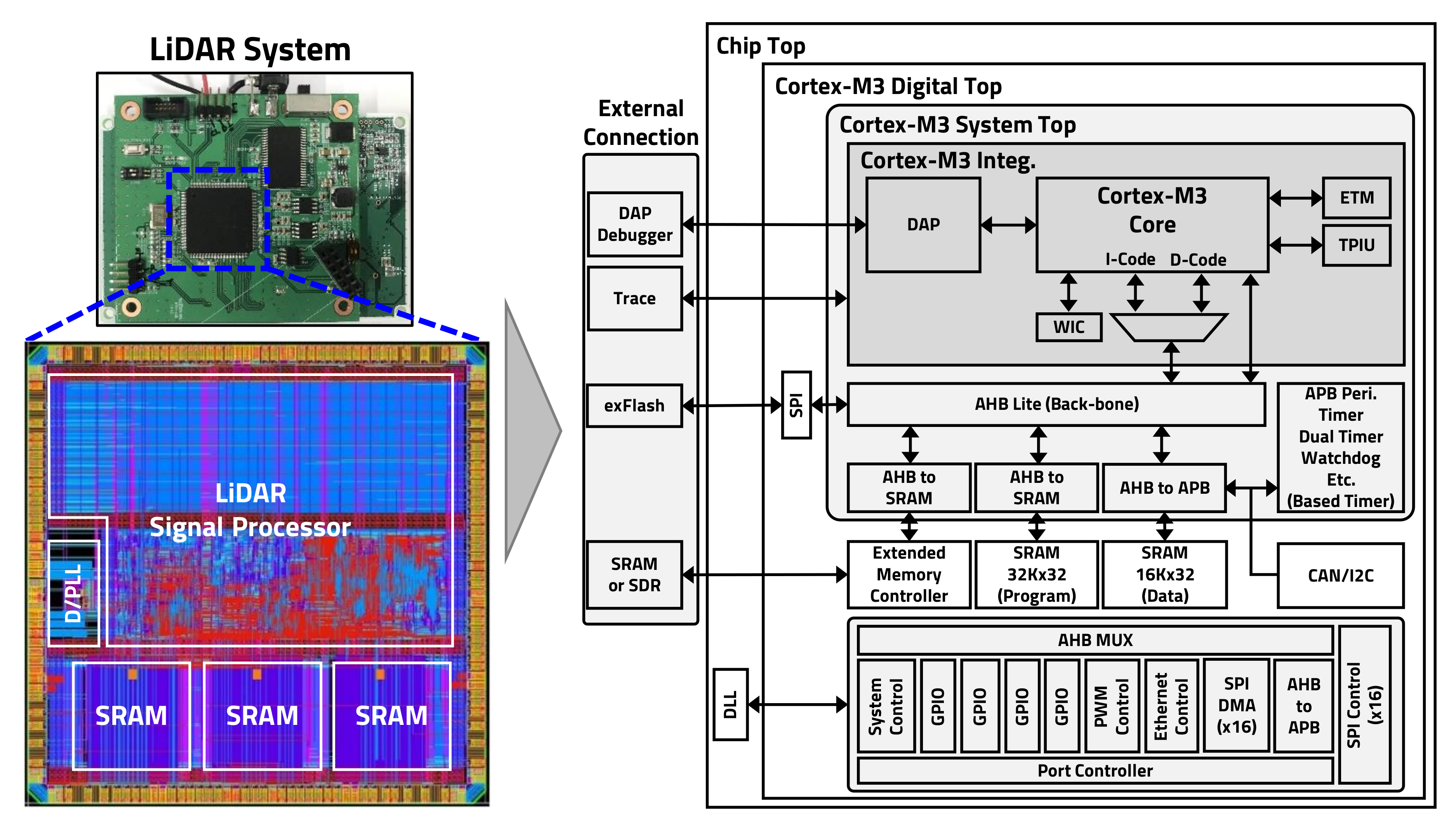
4.2. Chip Designed for the LiDAR Sensor
5. Conclusions
Author Contributions
Funding
Conflicts of Interest
Abbreviations
| LiDAR | light detection and ranging |
| HAR | horizontal angular resolution |
| LD | laser diode |
| NIR | near-infrared ray |
| ToF | time-of-flight |
| APD | avalanche photo diode |
| TDC | time-to-digital converter |
| MP | microprocessor |
| AMCW | amplitude-modulated continuous-wave |
| FMCW | frequency-modulated continuous-wave |
| MEMS | microelectromechanical systems |
| OPA | optical phased array |
| RADAR | radio detection and ranging |
| VAR | vertical angular resolution |
| BLDC | brushless direct current |
| VFoV | vertical field of view |
| PWM | pulse width modulation |
| TMR | internal timer |
| HFoV | horizontal field of view |
| SPI | serial peripheral interface |
| OSC | oscillator |
| BRR | BroadR-Reach ethernet |
| CAN | controller area network |
| ECU | engine control unit |
| PCL | point cloud library |
| AC | average current |
| APC | average power consumption |
| DAC | difference in average current |
| DAPC | difference in average power consumption |
| PRR | power reduction rate |
References
- Basu, A.K.; Tatiya, S.; Bhattacharya, S. Overview of Electric Vehicles (EVs) and EV Sensors. In Sensors for Automotive and Aerospace Applications; Springer: Singapore, 2019; pp. 107–122. [Google Scholar]
- Armstrong, K.; Das, S.; Cresko, J. The energy footprint of automotive electronic sensors. Sustain. Mater. Technol. 2020, 25, e00195. [Google Scholar]
- Winner, H.; Hakuli, S.; Lotz, F.; Singer, C. Handbook of Driver Assistance Systems; Springer International Publishing: Amsterdam, The Netherlands, 2014; pp. 405–430. [Google Scholar]
- Rasshofer, R.; Gresser, K. Automotive Radar and Lidar Systems for Next Generation Driver Assistance Functions. Adv. Radio Sci. Kleinheubacher Berichte 2005, 3, 205–209. [Google Scholar] [CrossRef] [Green Version]
- Jo, K.; Kim, J.; Kim, D.; Jang, C.; Sunwoo, M. Development of Autonomous Car-Part I: Distributed System Architecture and Development Process. IEEE Trans. Ind. Electron. 2014, 61, 7131–7140. [Google Scholar] [CrossRef]
- Hecht, J. Lidar for Self-Driving Cars. Opt. Photonics News 2018, 29, 26–35. [Google Scholar] [CrossRef]
- Crouch, S. Advantages of 3D imaging coherent lidar for autonomous driving applications. In Proceedings of the 19th Coherent Laser Radar Conference, Okinawa, Japan, 18–21 June 2018. [Google Scholar]
- Sarbolandi, H.; Plack, M.; Kolb, A. Pulse Based Time-of-Flight Range Sensing. Sensors 2018, 18, 1679. [Google Scholar] [CrossRef] [Green Version]
- Theiß, S. Analysis of a Pulse-Based ToF Camera for Automotive Application. Master’s Thesis, University of Siegen, Siegen, Germany, 27 March 2015. [Google Scholar]
- Gokturk, S.; Yalcin, H.; Bamji, C. A Time-Of-Flight Depth Sensor-System Description, Issues and Solutions. In Proceedings of the 2004 IEEE Computer Society Conference on Computer Vision and Pattern Recognition, CVPR 2004, Washington, DC, USA, 27 June–2 July 2004; p. 35. [Google Scholar]
- Amann, M.C.; Bosch, T.; Lescure, M.; Myllyla, R.; Rioux, M. Laser Ranging: A Critical Review of Unusual Techniques for Distance Measurement. Opt. Eng. 2001, 40, 10–19. [Google Scholar]
- Behroozpour, B.; Sandborn, P.; Wu, M.; Boser, B. Lidar System Architectures and Circuits. IEEE Commun. Mag. 2017, 55, 135–142. [Google Scholar] [CrossRef]
- Agishev, R.; Gross, B.; Moshary, F.; Gilerson, A.; Ahmed, S. Range-resolved pulsed and CWFM lidars: Potential capabilities comparison. Appl. Phys. B 2006, 85, 149–162. [Google Scholar] [CrossRef]
- Feneyrou, P.; Leviandier, L.; Minet, J.; Pillet, G.; Martin, A.; Dolfi, D.; Schlotterbeck, J.P.; Rondeau, P.; Lacondemine, X.; Rieu, A.; et al. Frequency-modulated multifunction lidar for anemometry, range finding, and velocimetry—1. Theory and signal processing. Appl. Opt. 2017, 56, 9663–9675. [Google Scholar] [CrossRef]
- Thakur, R. Scanning LIDAR in Advanced Driver Assistance Systems and Beyond. IEEE Consum. Electron. Mag. 2016, 5, 48–54. [Google Scholar] [CrossRef]
- Mizuno, T.; Mita, M.; Kajikawa, Y.; Takeyama, N.; Ikeda, H.; Kawahara, K. Study of two-dimensional scanning LIDAR for planetary explorer. Proc. SPIE 2008, 7106. [Google Scholar] [CrossRef]
- Yoo, H.; Druml, N.; Brunner, D.; Schwarzl, C.; Thurner, T.; Hennecke, M.; Schitter, G. MEMS-based lidar for autonomous driving. e & i Elektrotechnik und Informationstechnik 2018, 135, 408–415. [Google Scholar] [CrossRef] [Green Version]
- Urey, H.; Holmstrom, S.; Baran, U. MEMS laser scanners: A review. J. Microelectromech. Syst. 2014, 23, 259–275. [Google Scholar]
- Moss, R.; Yuan, P.; Bai, X.; Quesada, E.; Sudharsanan, R.; Stann, B.; Dammann, J.; Giza, M.; Lawler, W. Low-cost compact MEMS scanning LADAR system for robotic applications. Proc. SPIE 2012, 8379, 837903. [Google Scholar]
- Gelbart, A.; Redman, B.; Light, R.; Schwartzlow, C.; Griffis, A. Flash lidar based on multiple-slit streak tube imaging lidar. Proc. SPIE 2002, 4723, 9–19. [Google Scholar]
- Mcmanamon, P.; Banks, P.; Beck, J.; Huntington, A.; Watson, E. A comparison flash lidar detector options. Proc. SPIE 2016, 9832, 983202. [Google Scholar] [CrossRef] [Green Version]
- Sun, J.; Timurdogan, E.; Yaacobi, A.; Hosseini, E.; Watts, M. Large-scale nanophotonic phased array. Nature 2013, 493, 195–199. [Google Scholar] [CrossRef]
- Heck, M. Highly integrated optical phased arrays: Photonic integrated circuits for optical beam shaping and beam steering. Nanophotonics 2016, 6, 93–107. [Google Scholar] [CrossRef]
- Park, D.; Youn, J.M.; Cho, J. A low-power microcontroller with accuracy-controlled event-driven signal processing unit for rare-event activity-sensing iot devices. J. Sens. 2015, 2015. [Google Scholar] [CrossRef] [Green Version]
- Popa, C. Low-power low-voltage CMOS analog signal processing circuits using a functional core. In Proceedings of the 2016 IEEE International Conference on Electronics, Circuits and Systems (ICECS), Monte Carlo, Monaco, 11–14 December 2016; pp. 680–683. [Google Scholar]
- Malik, M.; Homayoun, H. Big data on low power cores: Are low power embedded processors a good fit for the big data workloads? In Proceedings of the 2015 33rd IEEE International Conference on Computer Design (ICCD), New York, NY, USA, 18–21 October 2015; pp. 379–382. [Google Scholar]
- Lorenzon, A.F.; Cera, M.C.; Beck, A.C.S. On the influence of static power consumption in multicore embedded systems. In Proceedings of the 2015 IEEE International Symposium on Circuits and Systems (ISCAS), Lisbon, Portugal, 24–27 May 2015; pp. 1374–1377. [Google Scholar]
- Lee, Y.; Park, M. Power Consumption and Accuracy in Detecting Pedestrian Images on Neuromorphic Hardware Accelerated Embedded Systems. In Proceedings of the 2019 Tenth International Green and Sustainable Computing Conference (IGSC), Alexandria, VA, USA, 21–24 October 2019; pp. 1–4. [Google Scholar]
- Anne, V.S.R.K.; Vadada, S.; Sharma, S.; Shareef, B.S.M.; Rao, C.H.S. Design challenges of a low power ARM based image processing sub system for a portable radar. In Proceedings of the 2017 2nd International Conference on Communication and Electronics Systems (ICCES), Coimbatore, India, 19–20 October 2017; IEEE: Piscataway, NJ, USA, 2017; pp. 193–198. [Google Scholar]
- Song, C.; Yavari, E.; Singh, A.; Boric-Lubecke, O.; Lubecke, V. Detection sensitivity and power consumption vs. operation modes using system-on-chip based doppler radar occupancy sensor. In Proceedings of the 2012 IEEE Topical Conference on Biomedical Wireless Technologies, Networks, and Sensing Systems (BioWireleSS), Santa Clara, CA, USA, 15–18 January 2012; pp. 17–20. [Google Scholar]
- Douillard, B.; Underwood, J.; Kuntz, N.; Vlaskine, V.; Quadros, A.; Morton, P.; Frenkel, A. On the segmentation of 3d LIDAR point clouds. In Proceedings of the 2011 IEEE International Conference on Robotics and Automation (ICRA), Shanghai, China, 9–13 May 2011; IEEE: Piscataway, NJ, USA, 2011; pp. 2798–2805. [Google Scholar]
- Himmelsbach, M.; Mueller, A.; Lüttel, T.; Wünsche, H.J. LIDAR-based 3D object perception. In Proceedings of the 1st International Workshop on Cognition for Technical Systems, Munich, Germany, 6–8 October 2008; Volume 1. [Google Scholar]
- Liu, J.; Sun, Q.; Fan, Z.; Jia, Y. TOF lidar development in autonomous vehicle. In Proceedings of the 2018 IEEE 3rd Optoelectronics Global Conference (OGC), Shenzhen, China, 4–7 September 2018; pp. 185–190. [Google Scholar]
- Comeron, A.; Munoz-Porcar, C.; Rocadenbosch, F.; Rodriguez-Gomez, A.; Sicard, M. Current Research in Lidar Technology Used for the Remote Sensing of Atmospheric Aerosols. Sensors 2017, 17, 1450. [Google Scholar] [CrossRef] [Green Version]
- Sun, H. A Practical Guide to Handling Laser Diode Beams; Springer: Cham, Switzerland, 2015; Volume 147. [Google Scholar]
- Arvani, F.; Carusone, T.C.; Rogers, E.S. Tdc sharing in spad-based direct time-of-flight 3d imaging applications. In Proceedings of the 2019 IEEE International Symposium on Circuits and Systems (ISCAS), Sapporo, Hokkaido, Japan, 26–29 May 2019; pp. 1–5. [Google Scholar]
- Alahdab, S.; Mäntyniemi, A.; Kostamovaara, J. Review of a time-to-digital converter (TDC) based on cyclic time domain successive approximation interpolator method with sub-ps-level resolution. In Proceedings of the 2013 IEEE Nordic-Mediterranean Workshop on Time-to-Digital Converters (NoMe TDC), Perugia, Italy, 3 October 2013; pp. 1–5. [Google Scholar]
- Song, J.; An, Q.; Liu, S. A high-resolution time-to-digital converter implemented in field-programmable-gate-arrays. IEEE Trans. Nucl. Sci. 2006, 53, 236–241. [Google Scholar] [CrossRef]


| Model | Features | Specification |
|---|---|---|
| 16 ch LiDAR | Channels | 16 ch (Parallel layers) |
| Technology | Pulsed ToF | |
| Source | NIR 905 nm | |
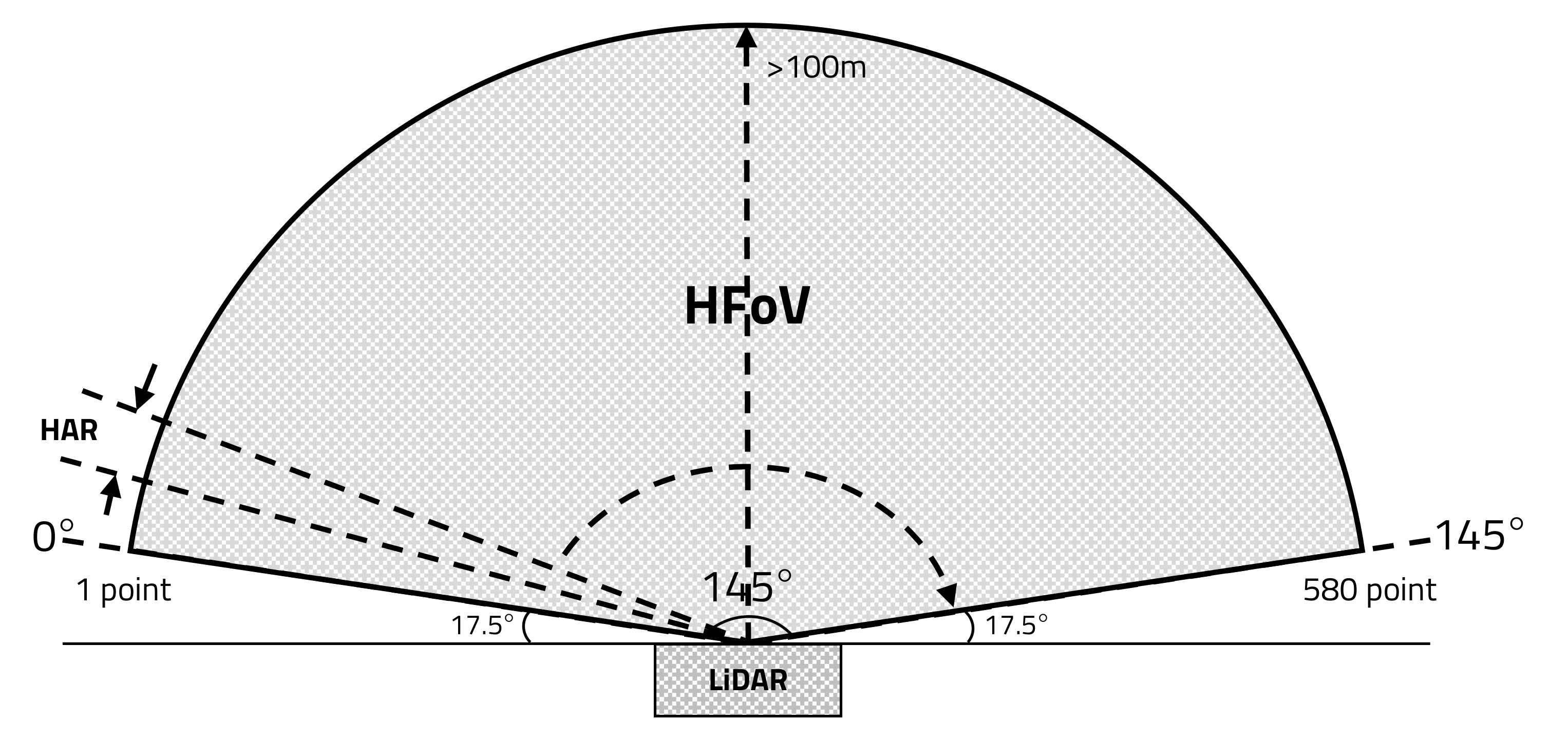
| HFoV | 145 | |
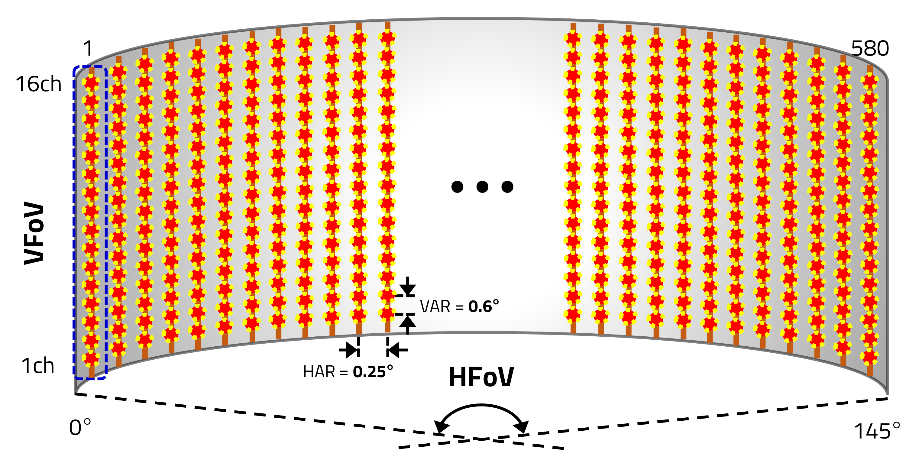
| VFoV | 9.6 | |
| Scanning frequency | 30 Hz | |
| Angular resolution | H : 0.25 / V : 0.6 | |
| Range | ≤150 | |
| Interface | BroadR–Reach Ethernet / CAN / RS–232 | |
| Viewer | Self-development using Qt | |
| Operation voltage | 10–36 VDC | |
| Power Consumption | ≤7.5 W |
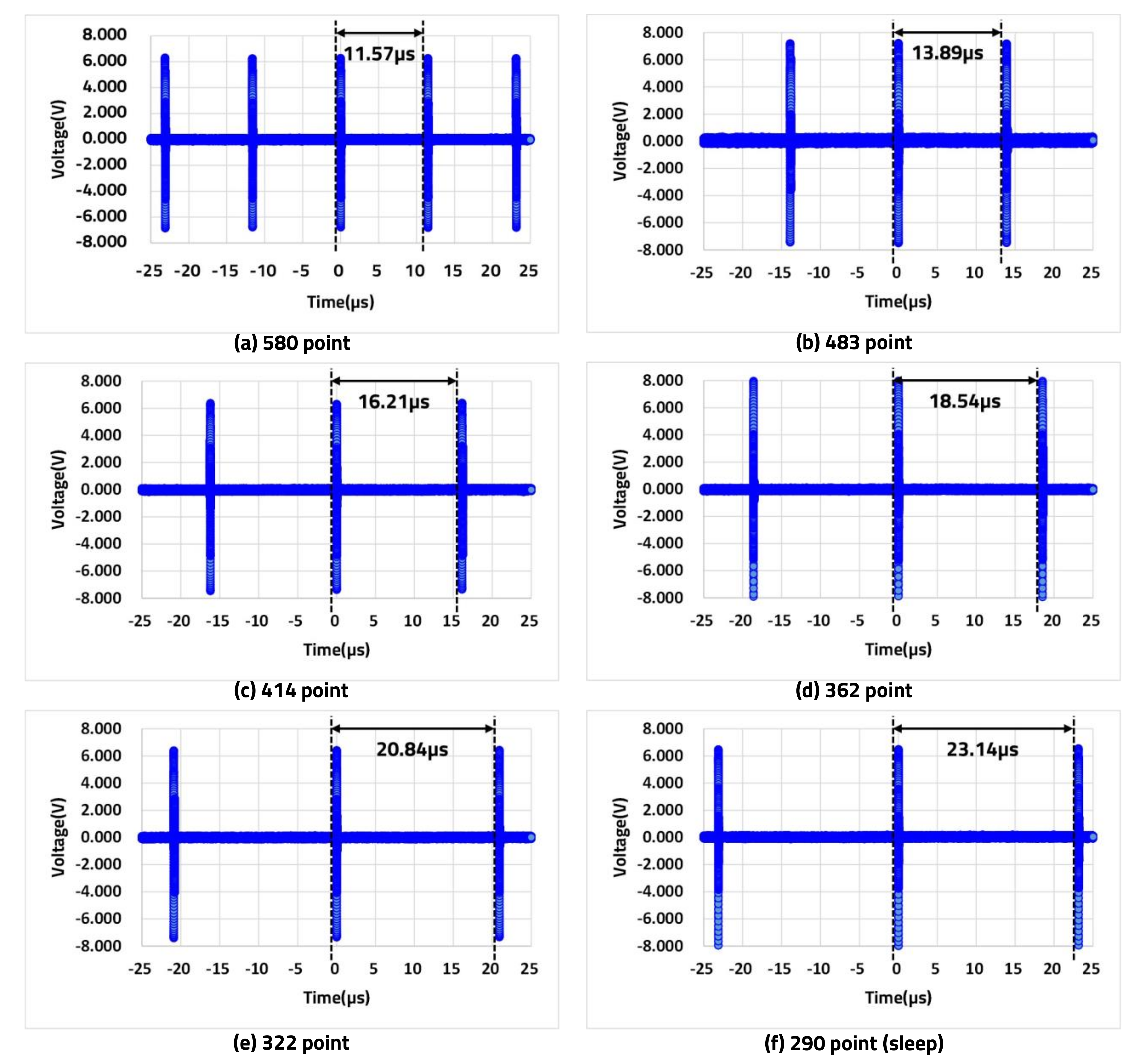
| HFoV () | HAR () | Term ( s) | |
|---|---|---|---|
| 145 | 0.25 | 580 | 11.57 |
| 0.3 | 483 | 13.89 | |
| 0.35 | 414 | 16.21 | |
| 0.4 | 362 | 18.54 | |
| 0.45 | 322 | 20.84 | |
| 0.5 | 290 | 23.14 |
| Speed (km/h) | HAR () | Rate (%) | |
|---|---|---|---|
| S ≥ 100 | 0.25 (–) | 580 (–) | 100 (–) |
| 100 > S ≥ 80 | 0.3 (+0.05) | 483 (–97) | 83.23 (–16.73) |
| 80 > S ≥ 60 | 0.35 (+0.1) | 414 (–166) | 71.38 (–28.62) |
| 60 > S ≥ 40 | 0.4 (+0.15) | 362 (–218) | 62.41 (–37.56) |
| 40 > S ≥ 0 | 0.45 (+0.2) | 322 (–258) | 55.52 (–44.48) |
| Sleep mode | 0.50 (+0.25) | 290 (–290) | 50 (–50.00) |
| Supply Voltage (V) | AC (A) | APC (W) | Reduction Rate (%) | |
|---|---|---|---|---|
| No-load | 12.054 | 0.578 | 6.971 | - |
| 580 | 12.055 | 0.617 | 7.442 | 100 (–) |
| 483 | 12.055 | 0.615 | 7.409 | 99.56 (–0.44) |
| 414 | 12.055 | 0.609 | 7.347 | 98.72 (–1.28) |
| 362 | 12.056 | 0.606 | 7.308 | 98.21 (–1.79) |
| 322 | 12.056 | 0.605 | 7.289 | 97.95 (–2.05) |
| Sleep mode | 12.057 | 0.593 | 7.154 | 96.14 (–3.86) |
| DAC (mA) | DAPC (mW) | PRR (%) | |
|---|---|---|---|
| 580 | 39.0 | 470.4 | 100 (–) |
| 483 | 36.3 | 437.8 | 93.08 (–6.92) |
| 414 | 31.1 | 375.4 | 79.80 (–20.20) |
| 362 | 27.9 | 337.1 | 71.67 (–28.33) |
| 322 | 26.3 | 317.9 | 67.57 (–32.43) |
| Sleep mode | 15.1 | 183.0 | 38.91 (–61.09) |
© 2020 by the authors. Licensee MDPI, Basel, Switzerland. This article is an open access article distributed under the terms and conditions of the Creative Commons Attribution (CC BY) license (http://creativecommons.org/licenses/by/4.0/).
Share and Cite
Lee, S.; Lee, D.; Choi, P.; Park, D. Accuracy–Power Controllable LiDAR Sensor System with 3D Object Recognition for Autonomous Vehicle. Sensors 2020, 20, 5706. https://doi.org/10.3390/s20195706
Lee S, Lee D, Choi P, Park D. Accuracy–Power Controllable LiDAR Sensor System with 3D Object Recognition for Autonomous Vehicle. Sensors. 2020; 20(19):5706. https://doi.org/10.3390/s20195706
Chicago/Turabian StyleLee, Sanghoon, Dongkyu Lee, Pyung Choi, and Daejin Park. 2020. "Accuracy–Power Controllable LiDAR Sensor System with 3D Object Recognition for Autonomous Vehicle" Sensors 20, no. 19: 5706. https://doi.org/10.3390/s20195706