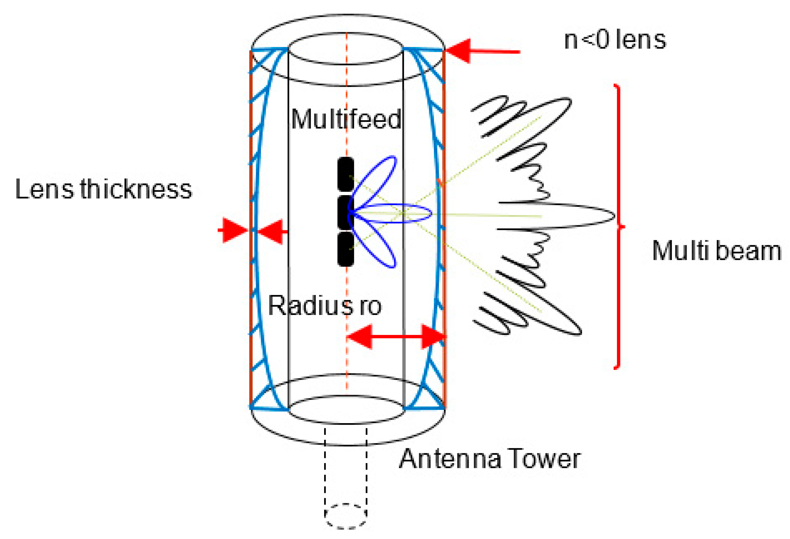
Figure 1.
Proposed mobile base station structure.
Figure 1.
Proposed mobile base station structure.
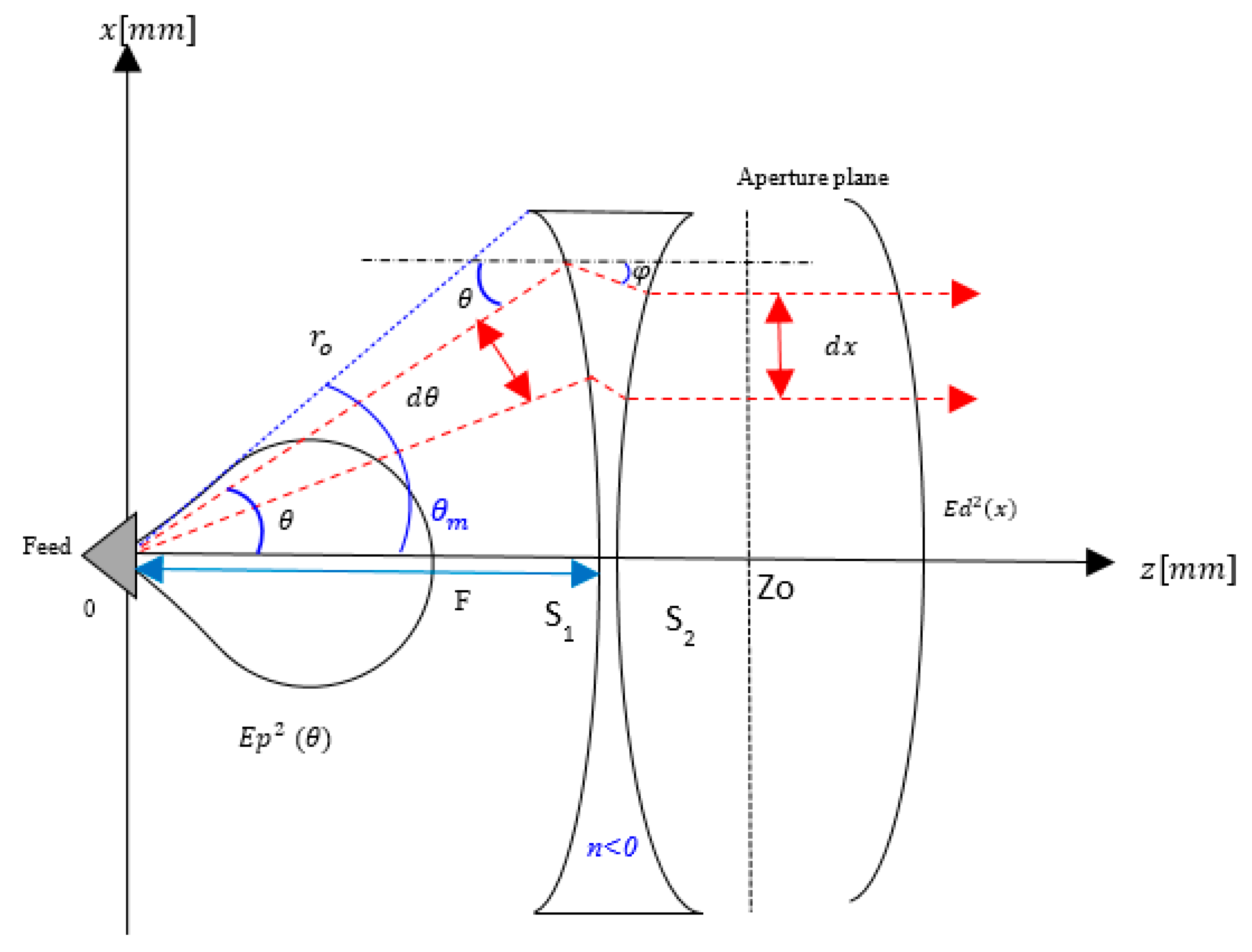
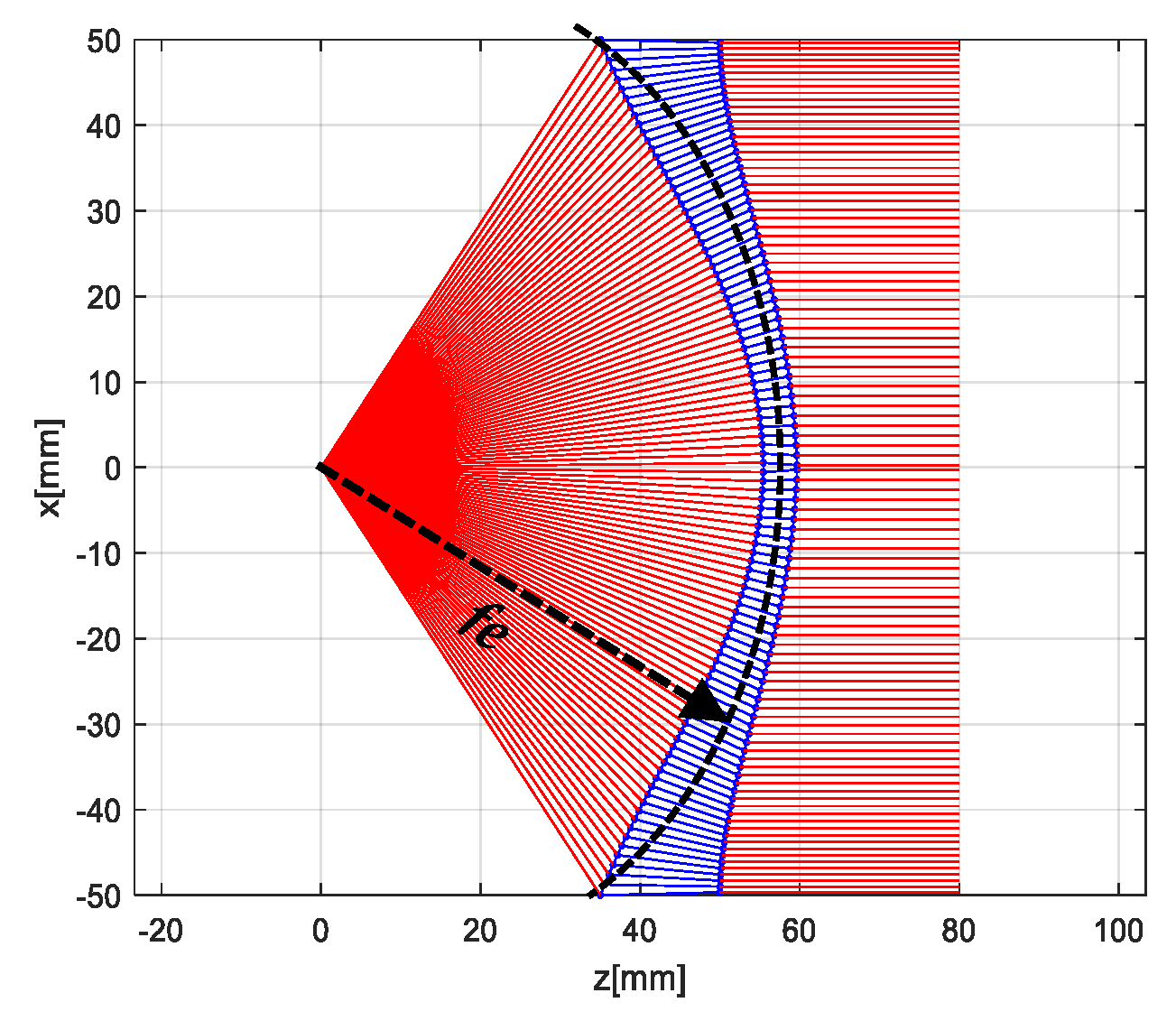
Figure 2.
Lens configuration and parameters.
Figure 2.
Lens configuration and parameters.
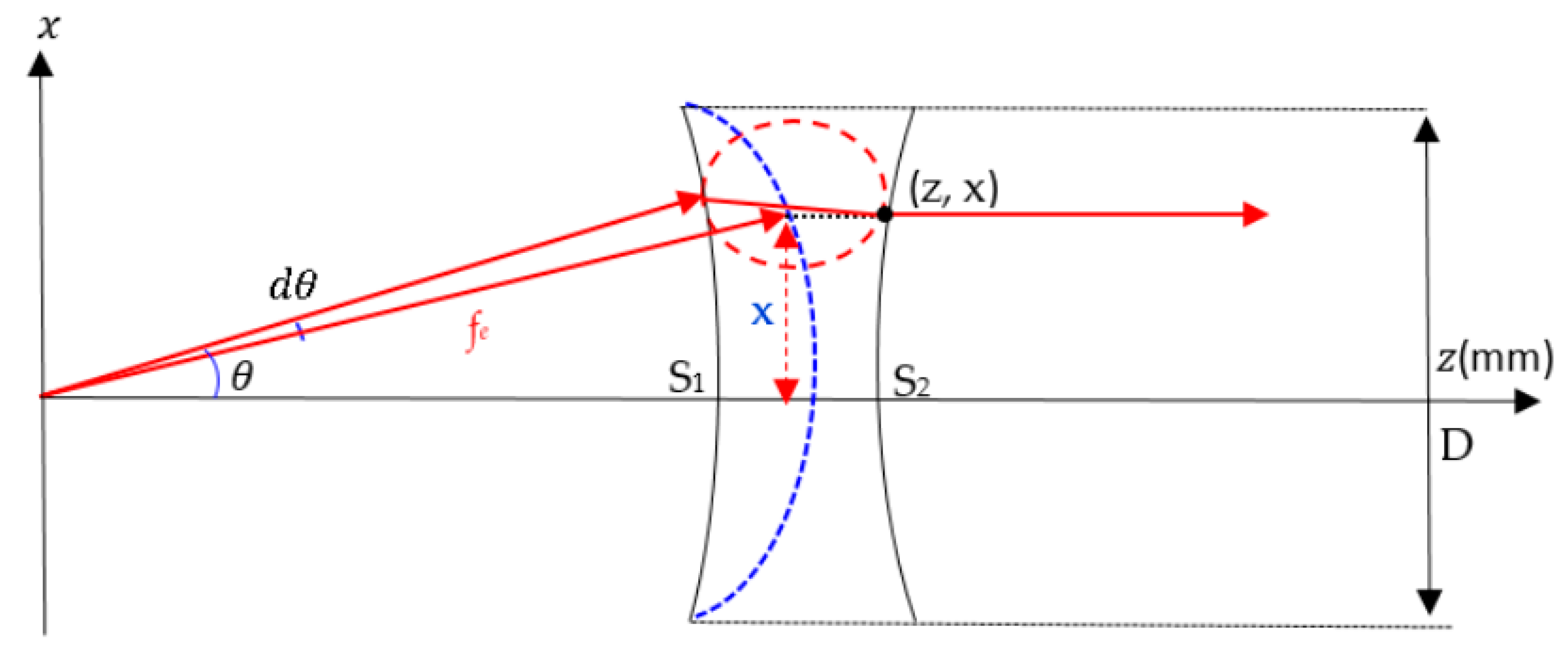
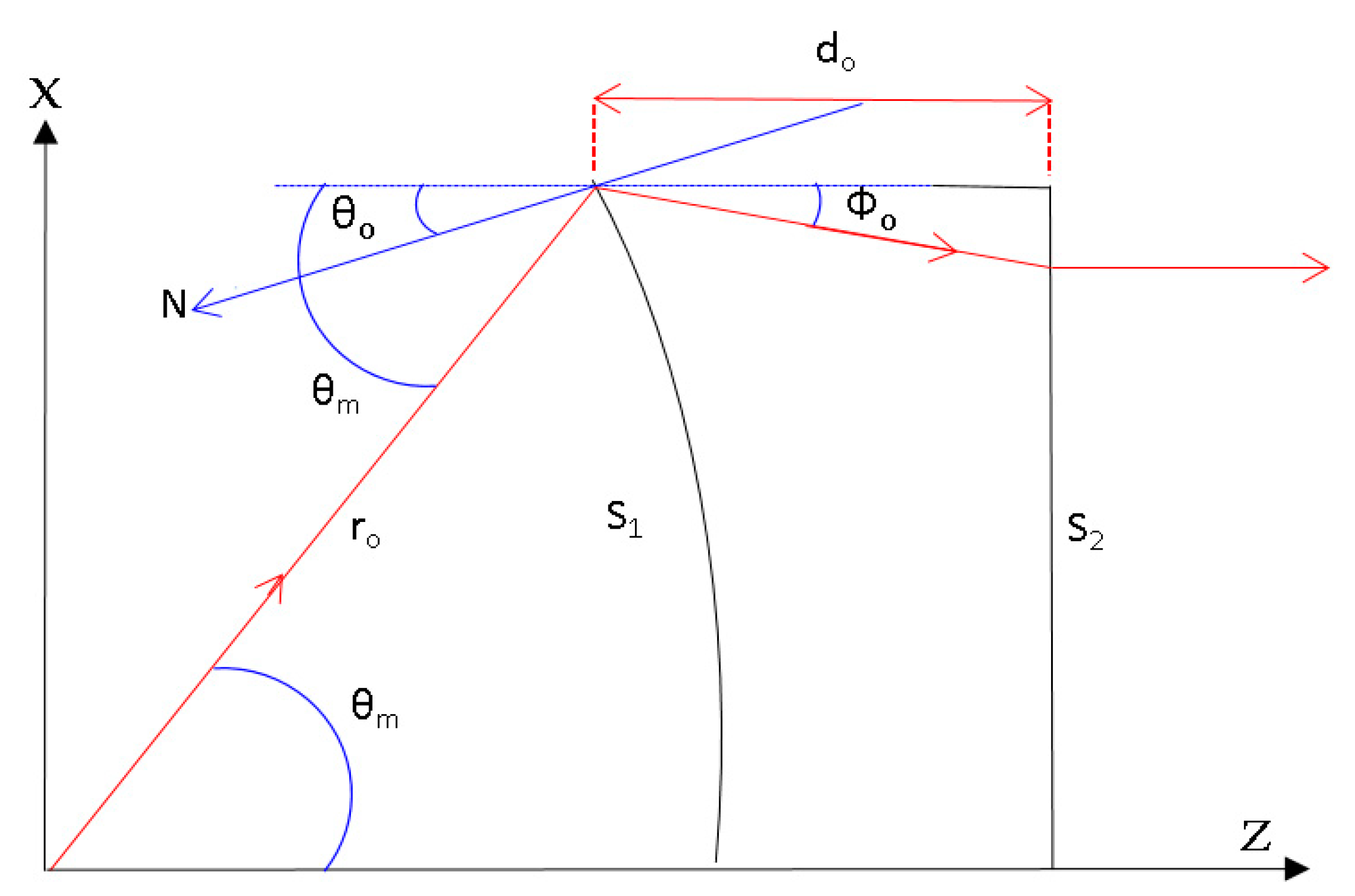
Figure 3.
Abbe’s sine condition.
Figure 3.
Abbe’s sine condition.
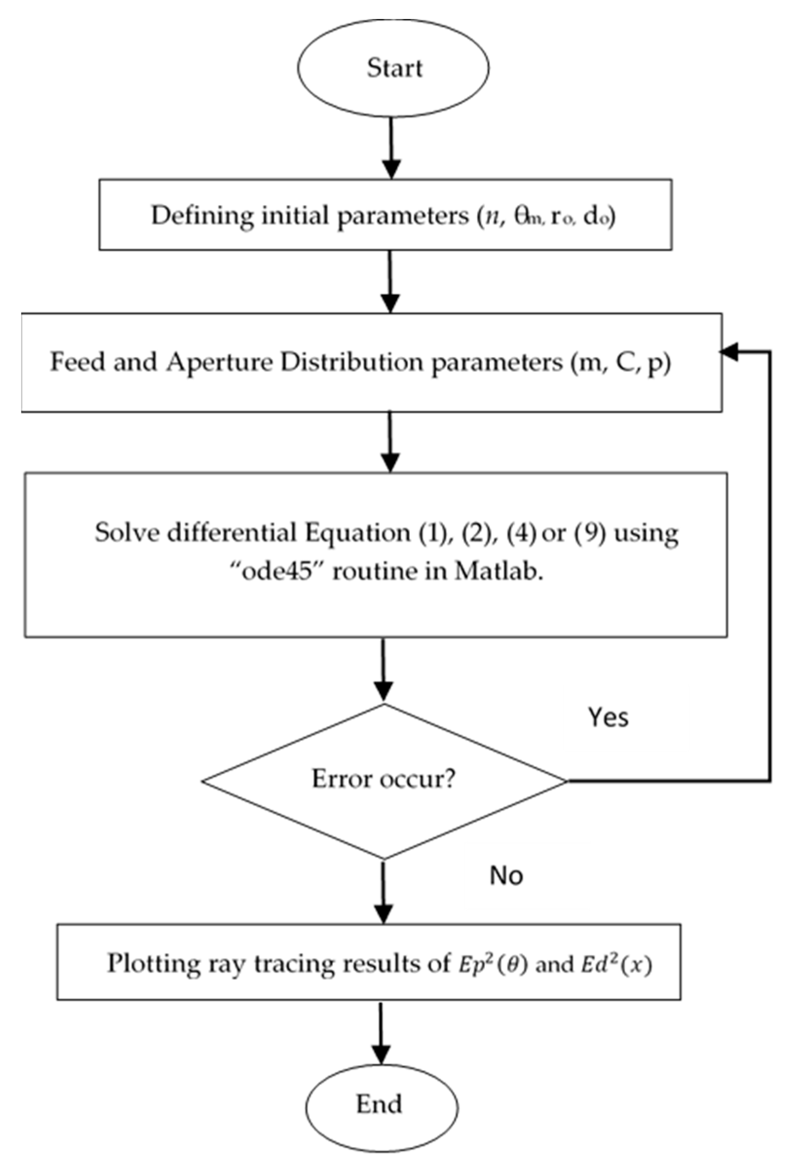
Figure 4.
MATLAB Program.
Figure 4.
MATLAB Program.
Figure 5.
Initial parameters at the lens edge.
Figure 5.
Initial parameters at the lens edge.
Figure 6.
Energy conservation design.
Figure 6.
Energy conservation design.
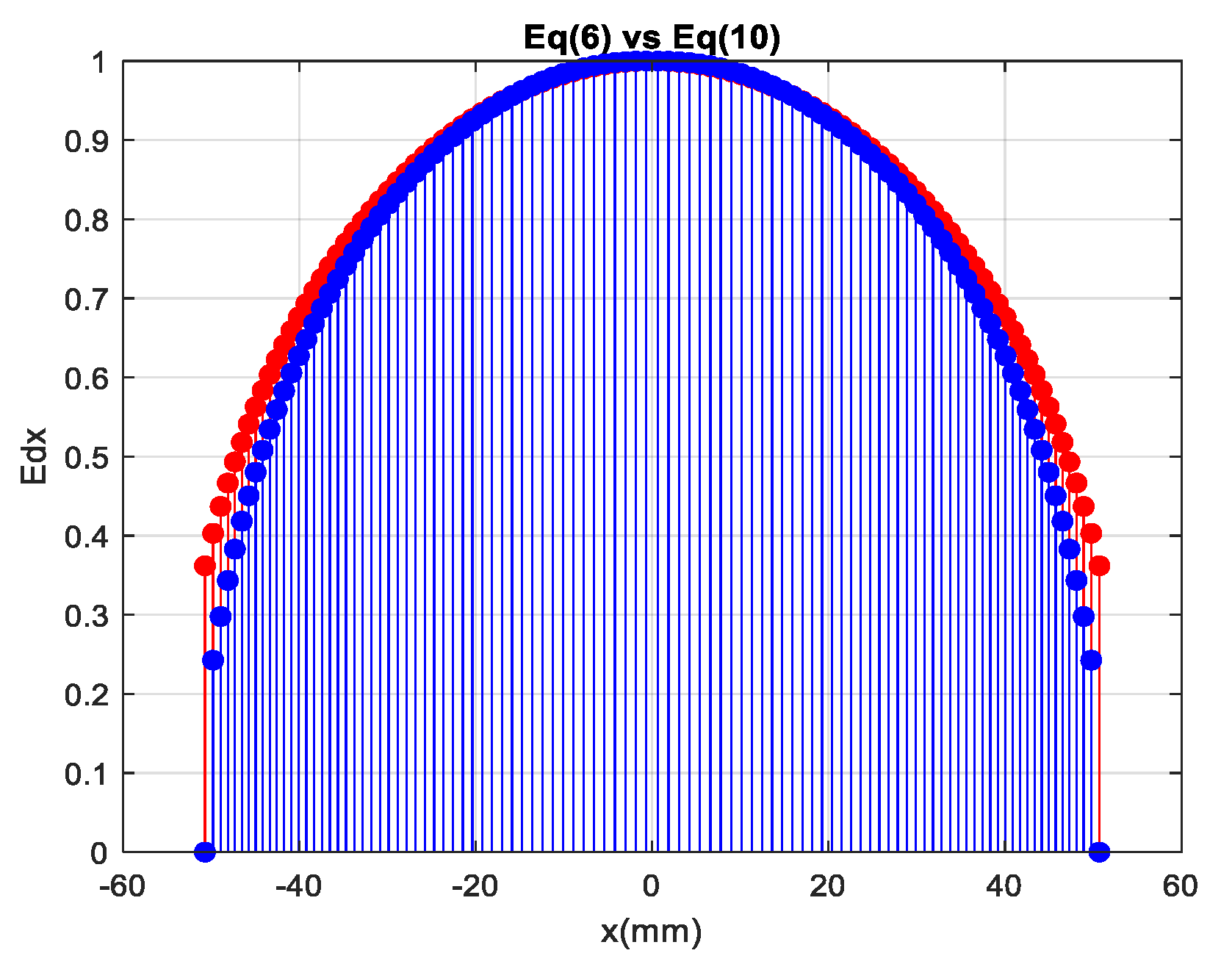
Figure 7.
Comparison of aperture distribution.
Figure 7.
Comparison of aperture distribution.
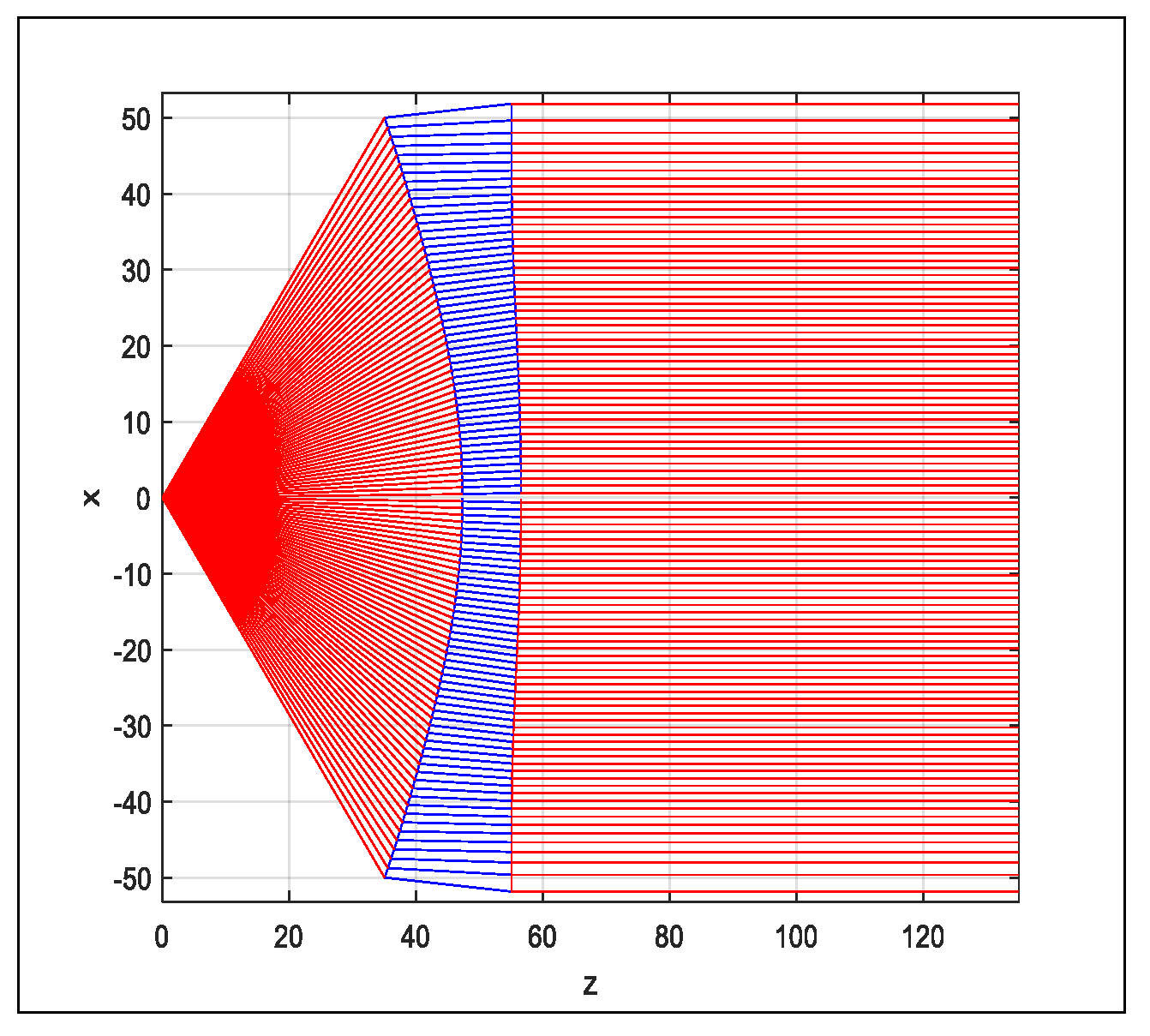
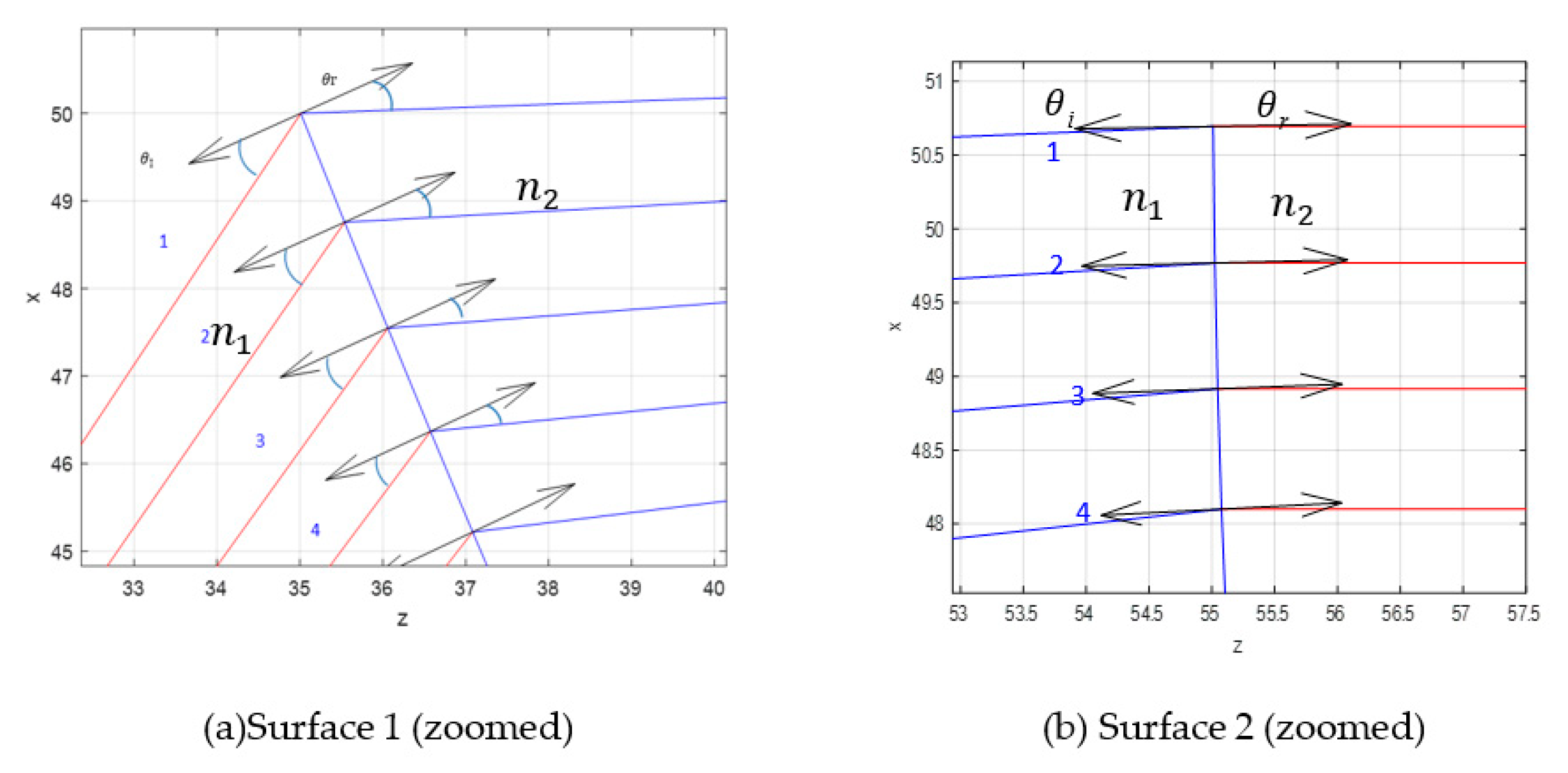
Figure 9.
Rays in and rays out.
Figure 9.
Rays in and rays out.
Figure 10.
Abbe’s sine shaped lens.
Figure 10.
Abbe’s sine shaped lens.
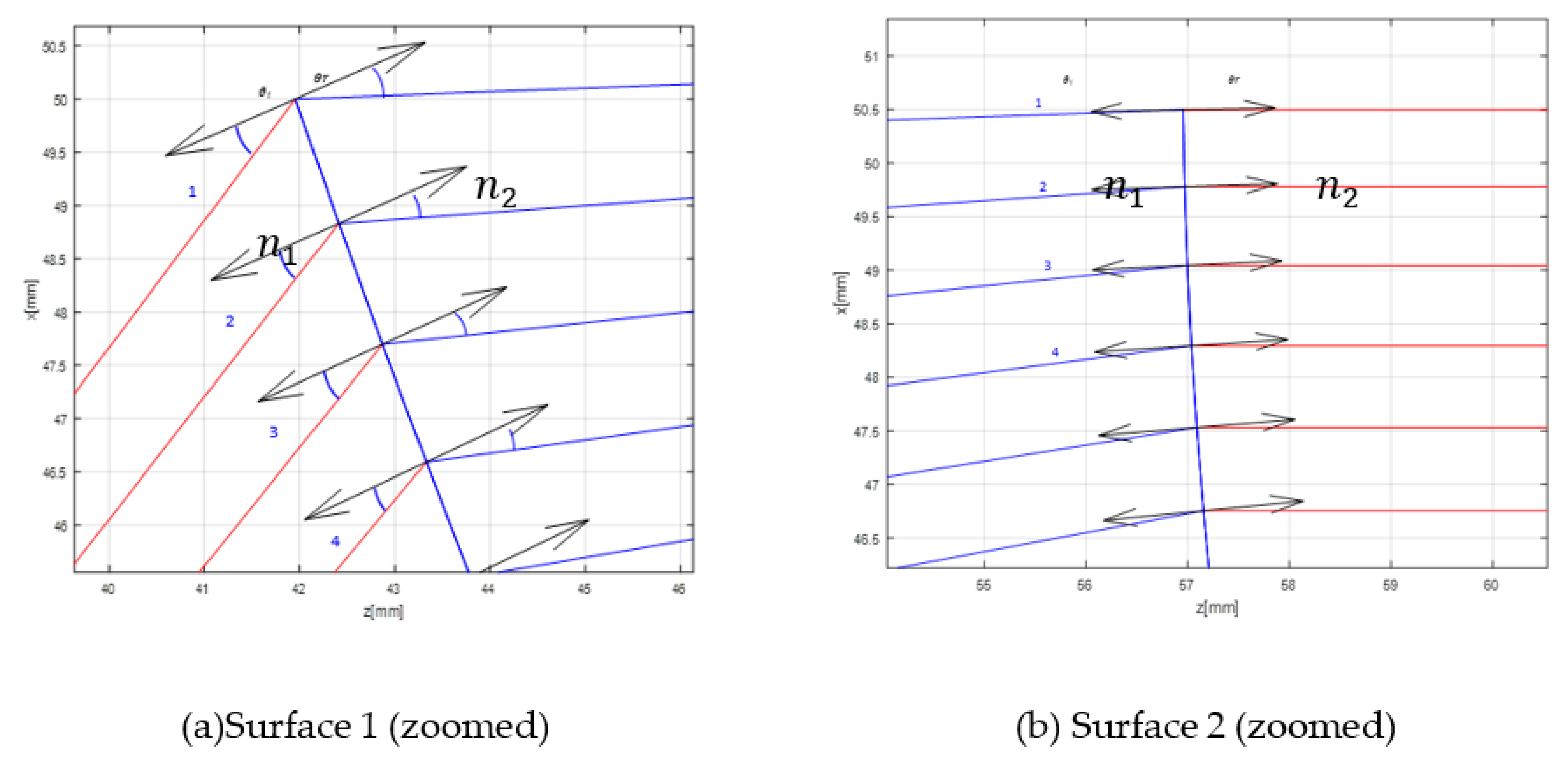
Figure 11.
Rays in and rays out.
Figure 11.
Rays in and rays out.
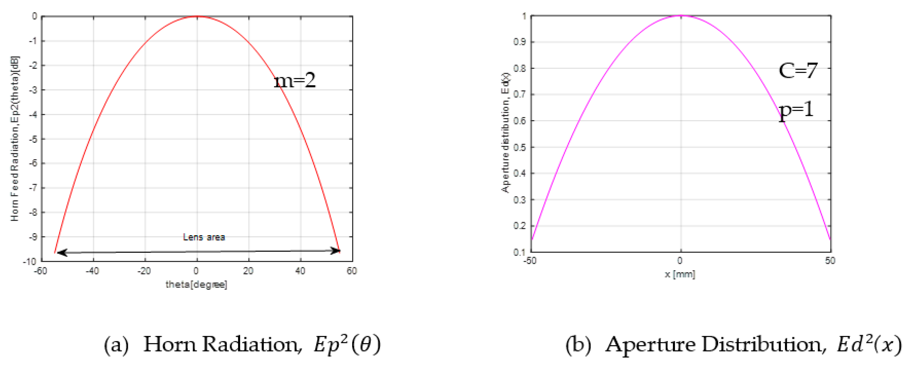
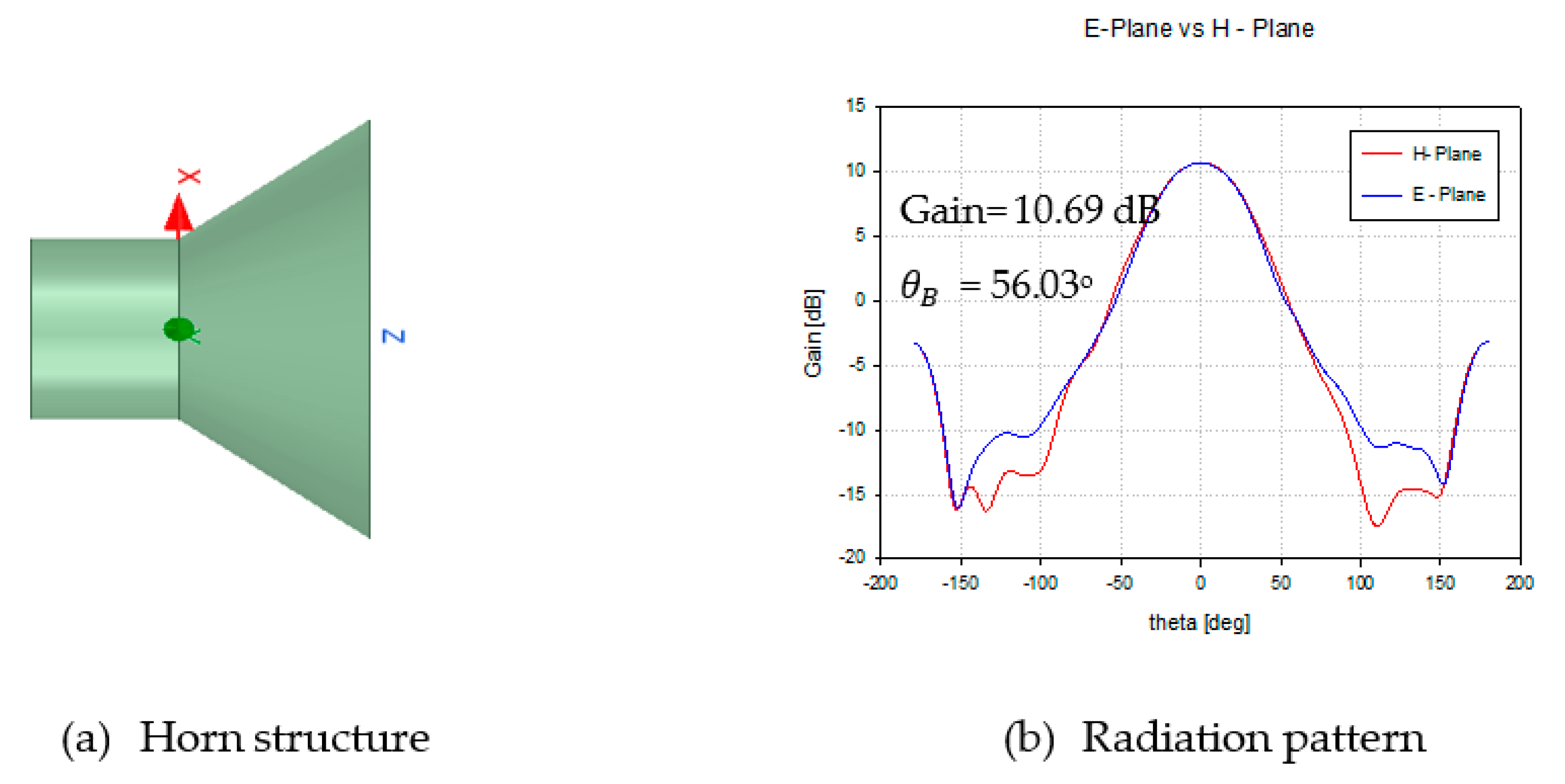
Figure 12.
Performance of horn antenna as a feed radiator.
Figure 12.
Performance of horn antenna as a feed radiator.
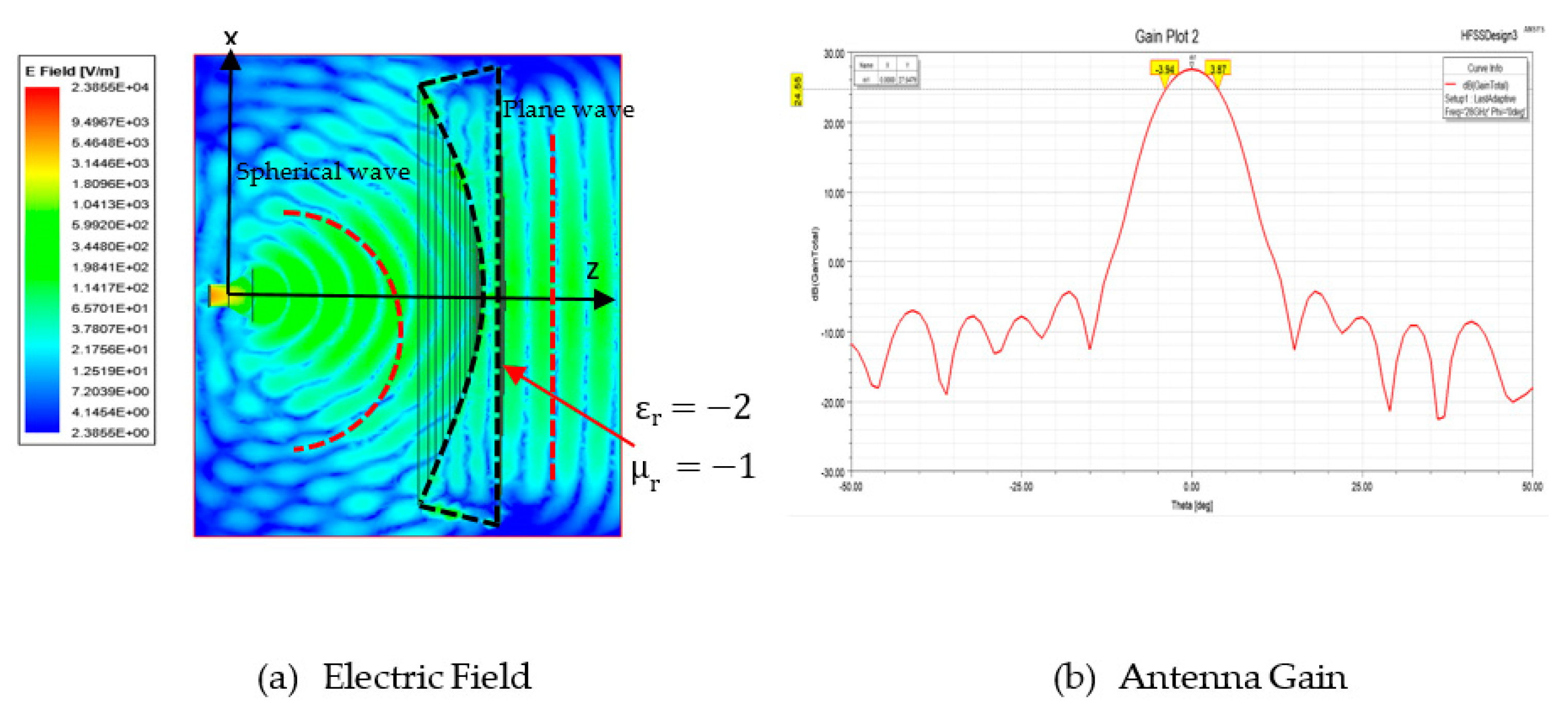
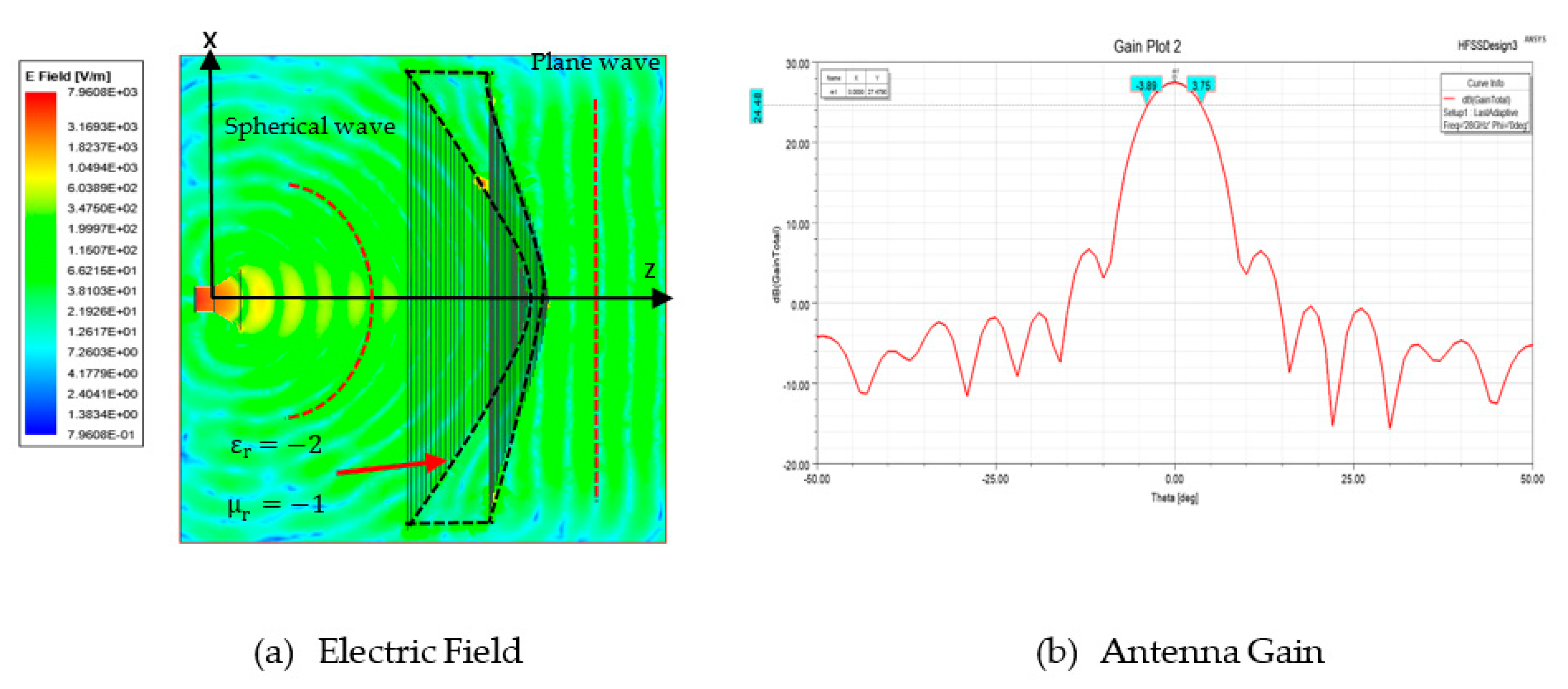
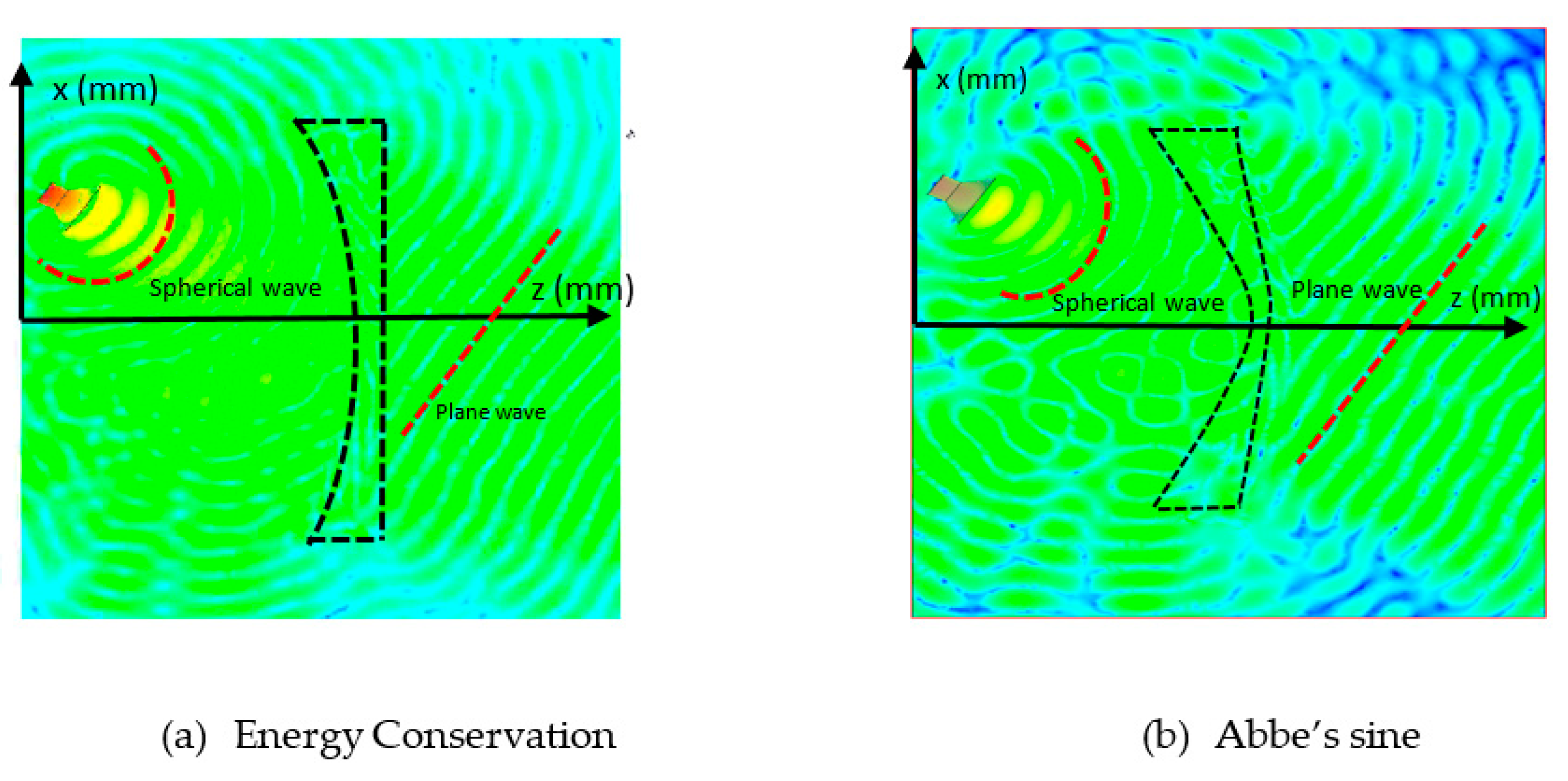
Figure 13.
Energy conservation shaped lens performance.
Figure 13.
Energy conservation shaped lens performance.
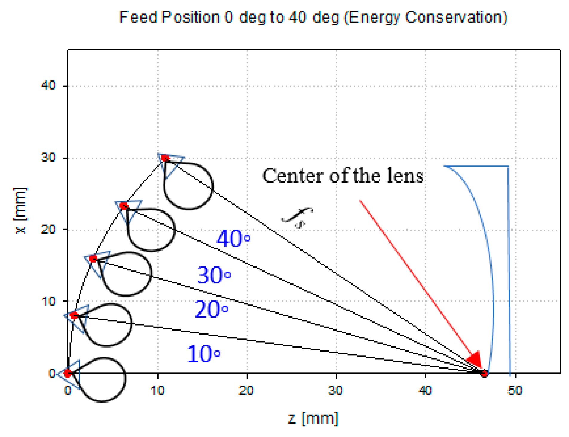
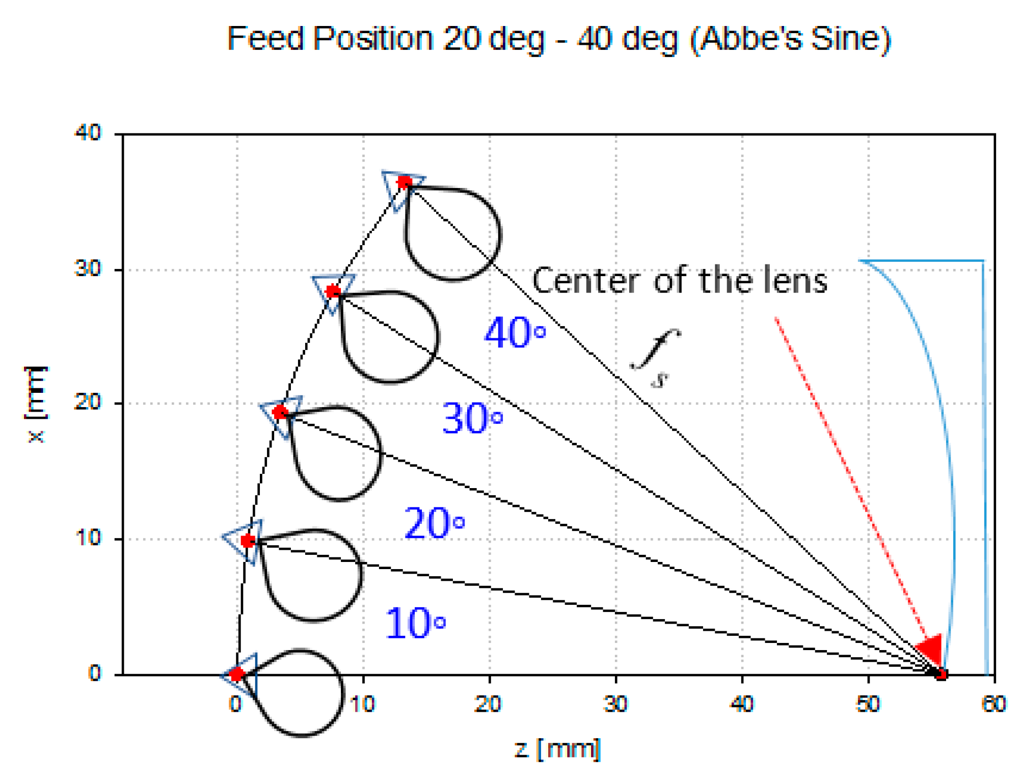
Figure 14.
Feed position arrangement.
Figure 14.
Feed position arrangement.
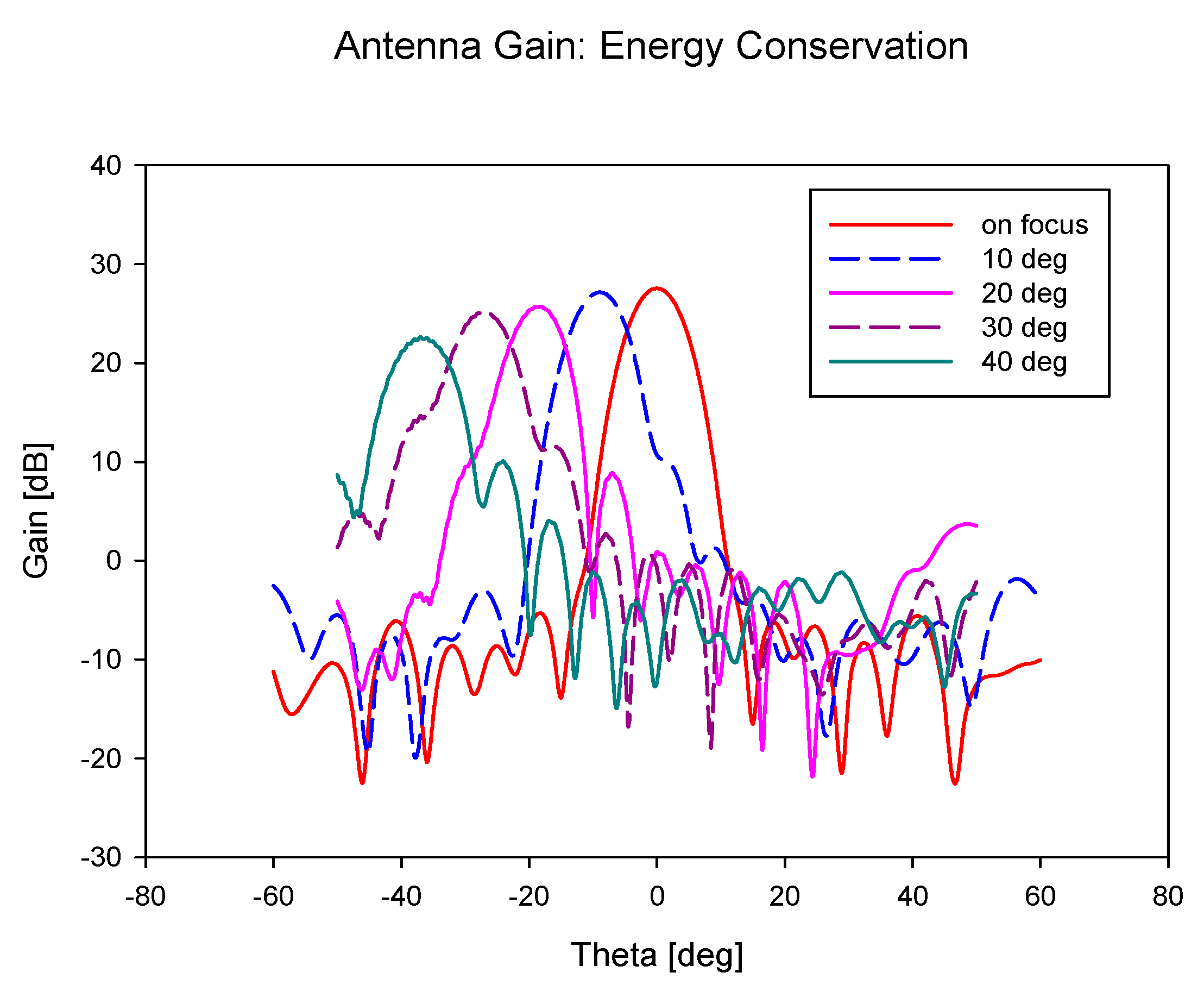
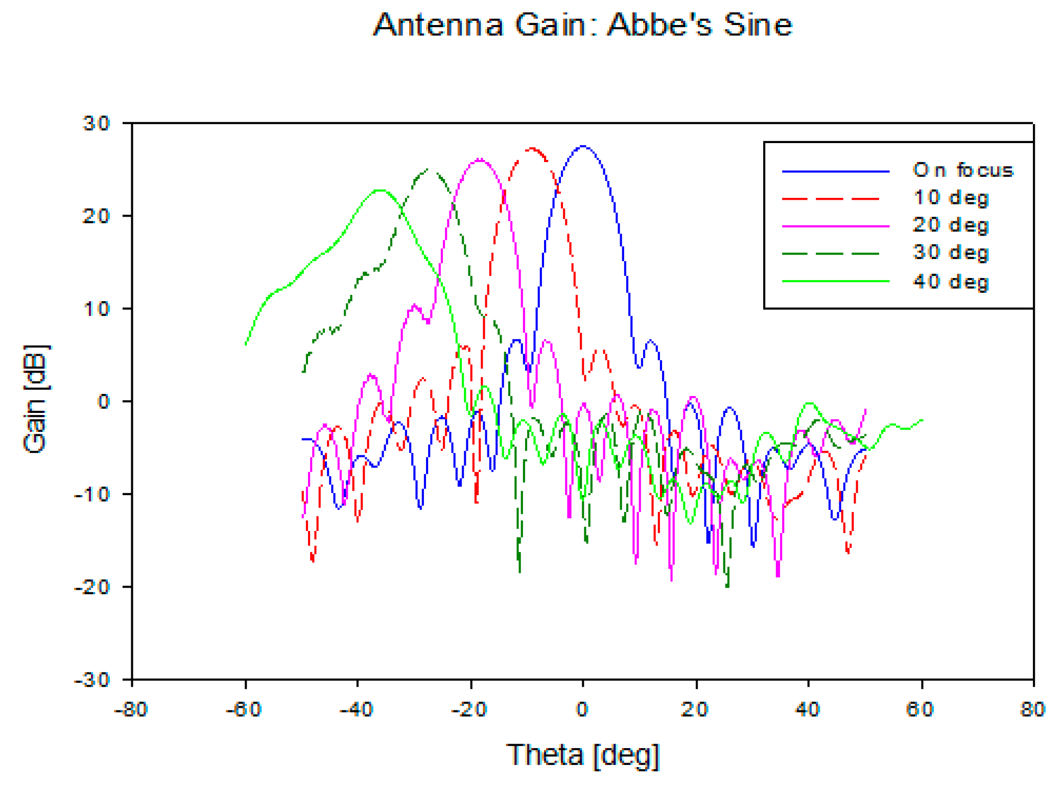
Figure 15.
Antenna gain for scanning angle 0° to 40°.
Figure 15.
Antenna gain for scanning angle 0° to 40°.
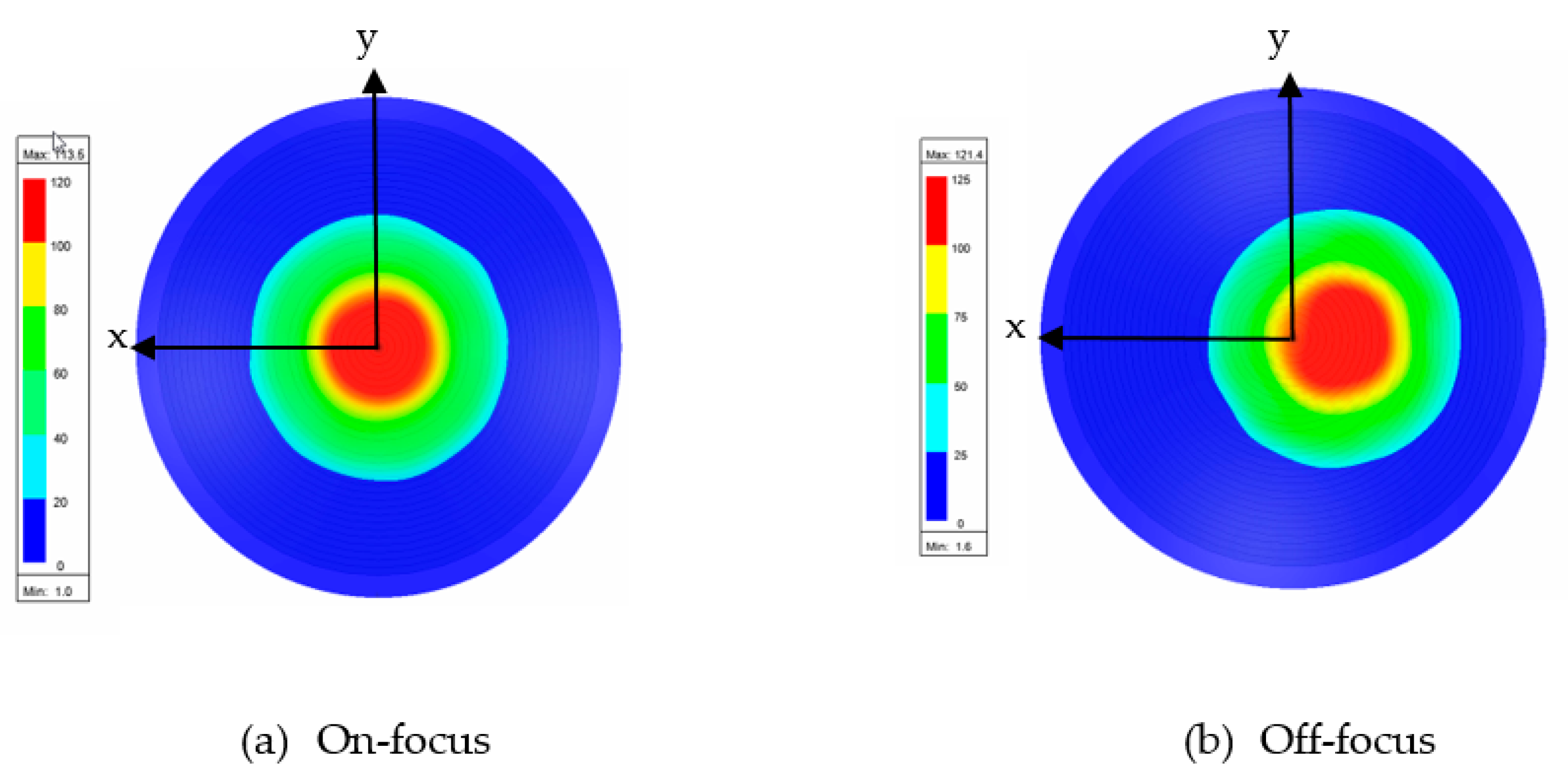
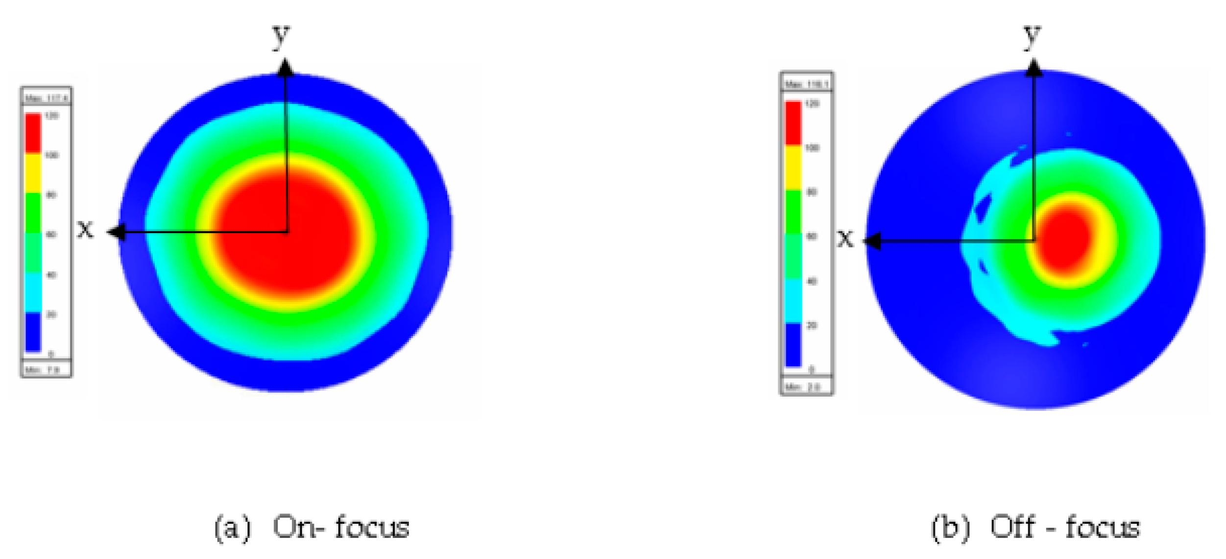
Figure 16.
Electric intensity distribution.
Figure 16.
Electric intensity distribution.
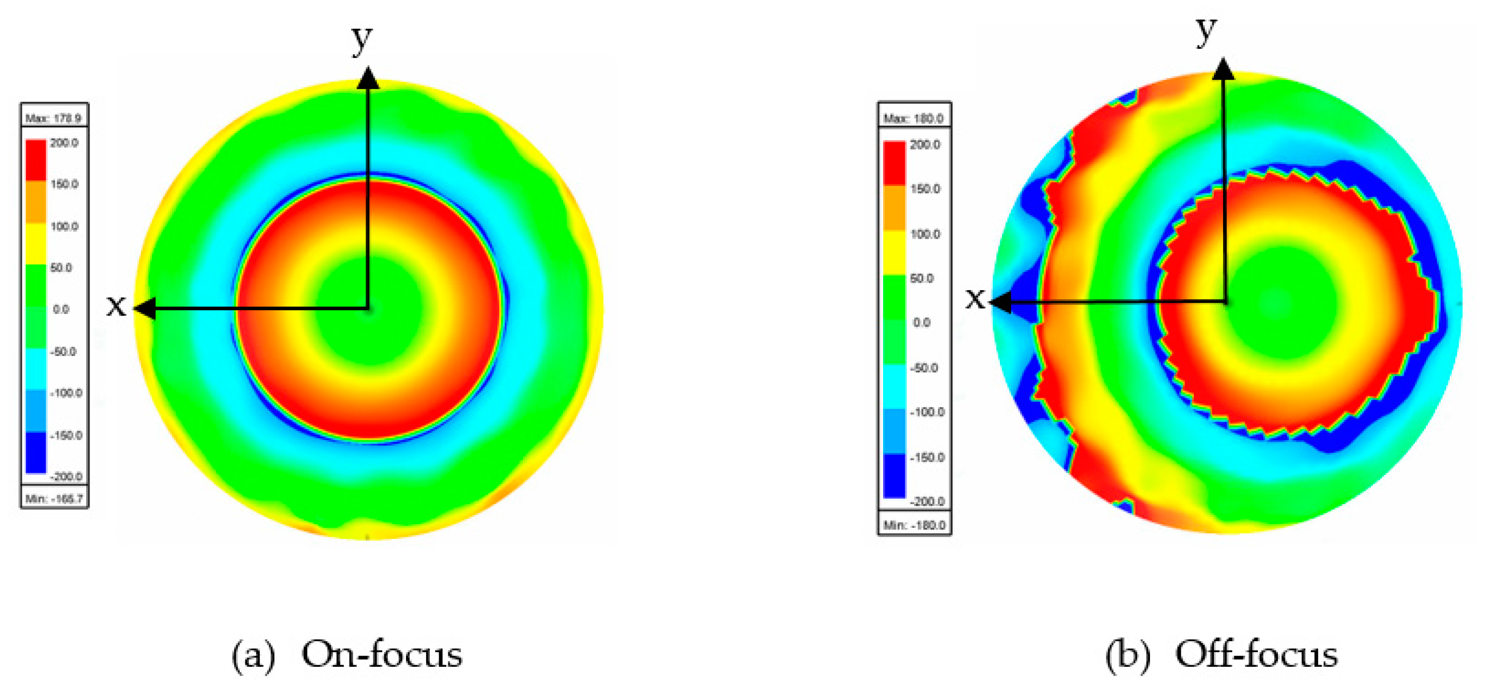
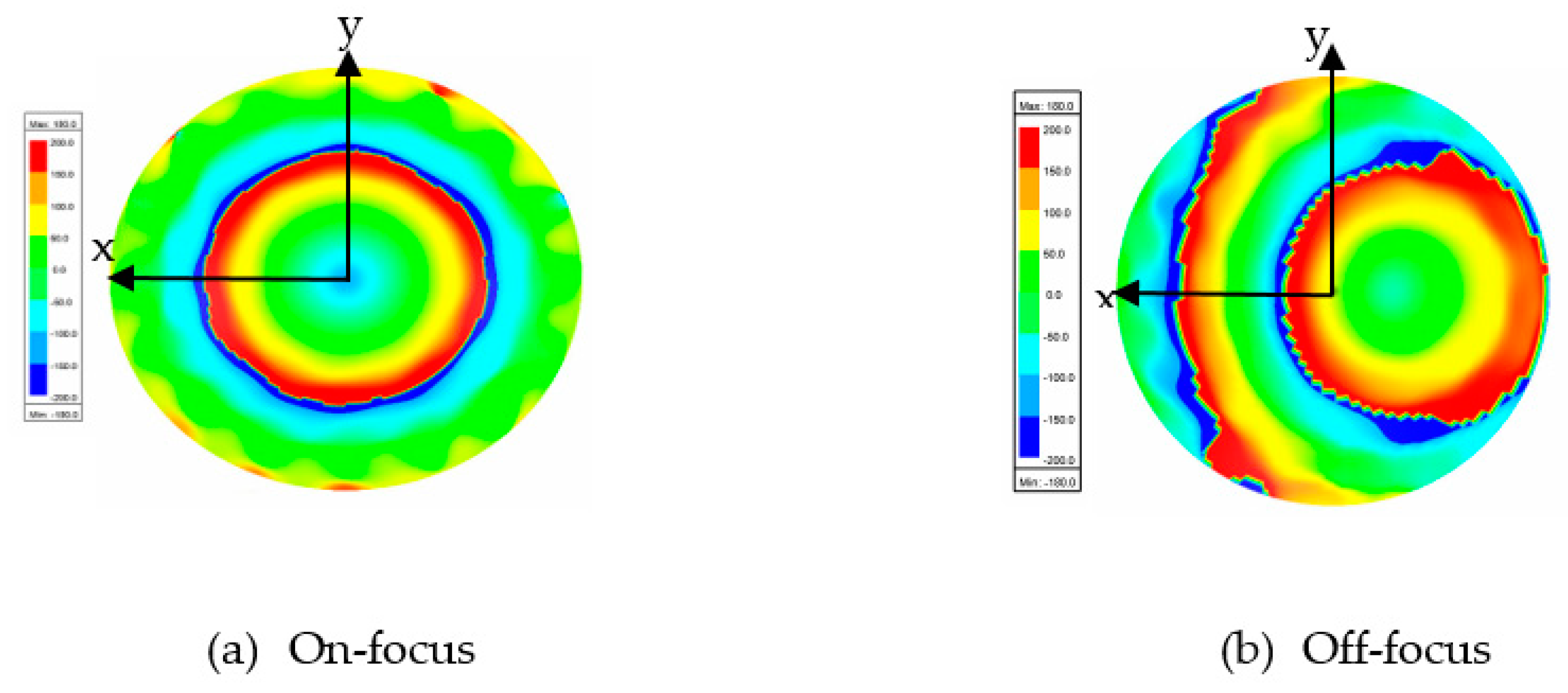
Figure 17.
Electric phase distribution.
Figure 17.
Electric phase distribution.
Figure 18.
Abbe’s sine shaped lens performance.
Figure 18.
Abbe’s sine shaped lens performance.
Figure 19.
Feed position arrangement.
Figure 19.
Feed position arrangement.
Figure 20.
Antenna gain for scanning angle 0° to 40°.
Figure 20.
Antenna gain for scanning angle 0° to 40°.
Figure 21.
Electric field distribution during off-focus.
Figure 21.
Electric field distribution during off-focus.
Figure 22.
Electric intensity distribution.
Figure 22.
Electric intensity distribution.
Figure 23.
Electric phase distribution.
Figure 23.
Electric phase distribution.
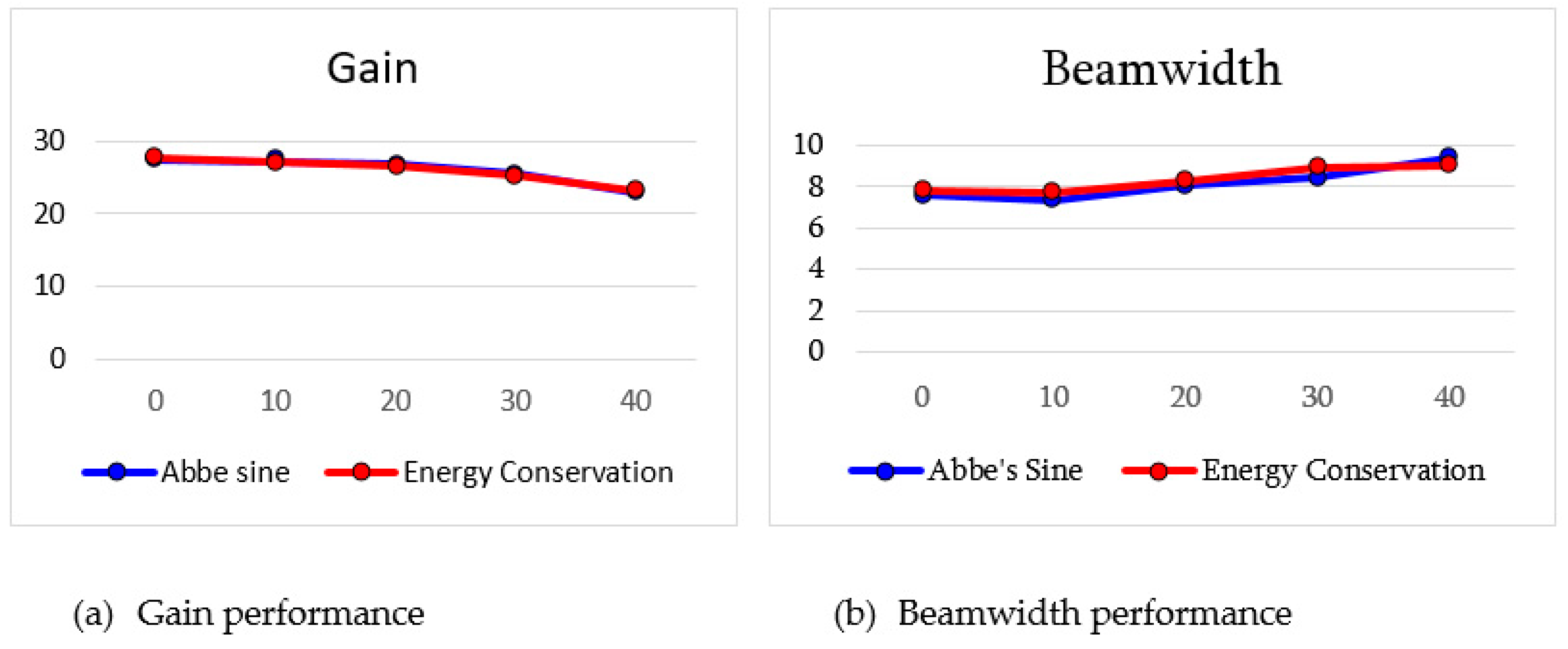
Figure 24.
Performance comparison for both types of lens.
Figure 24.
Performance comparison for both types of lens.
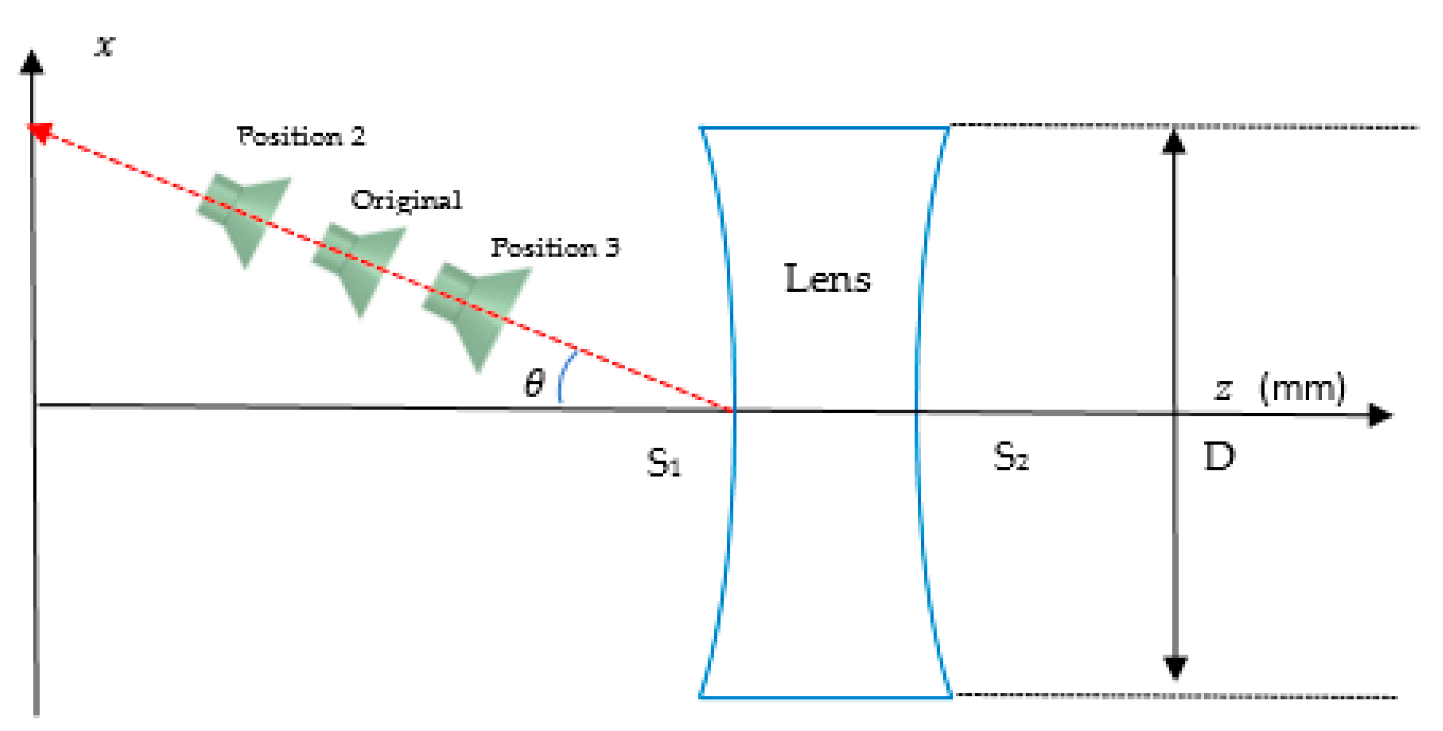
Figure 25.
Feed position analysis arrangement.
Figure 25.
Feed position analysis arrangement.
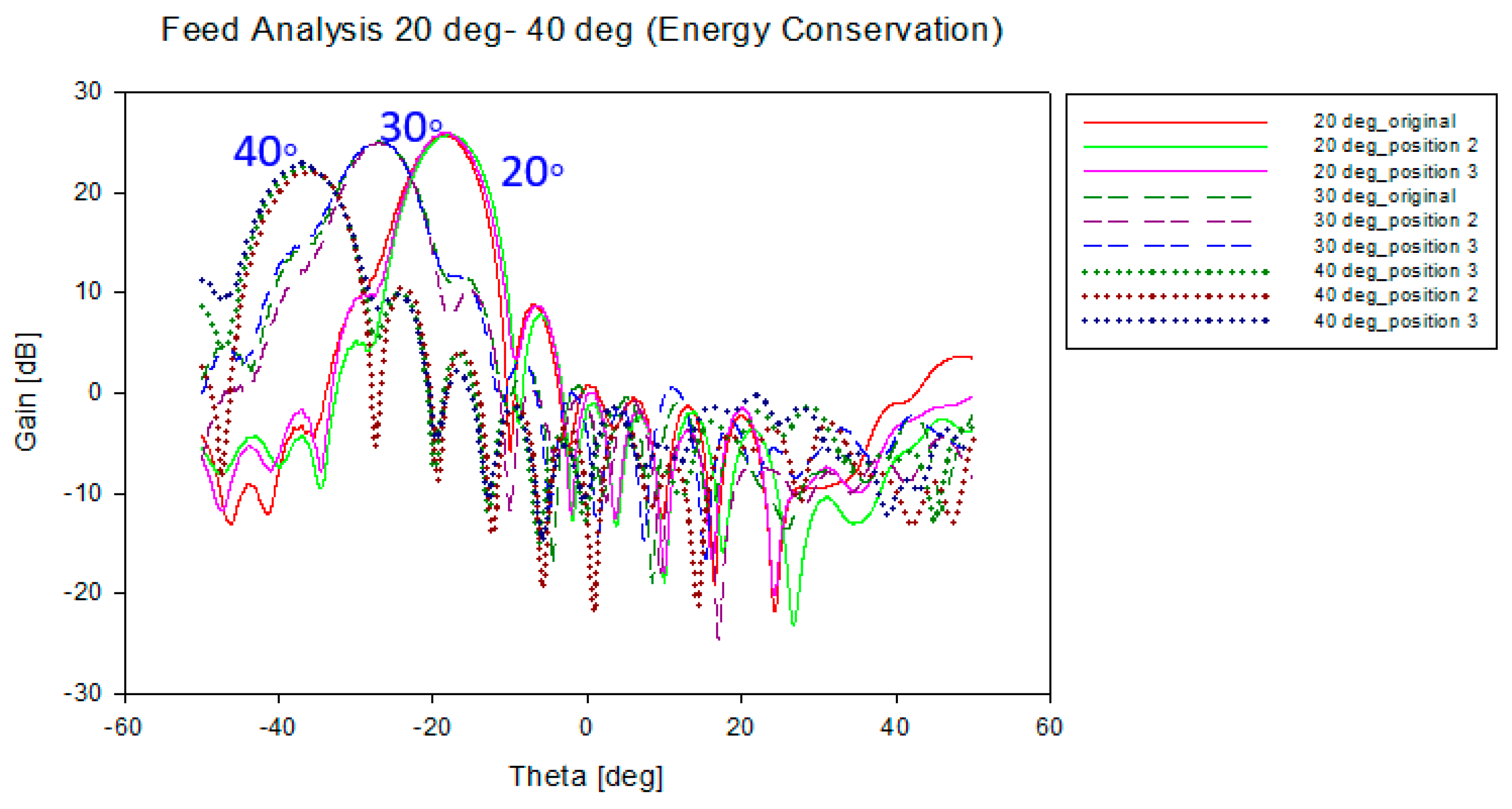
Figure 26.
Antenna gain for all feed position for energy conservation lens.
Figure 26.
Antenna gain for all feed position for energy conservation lens.
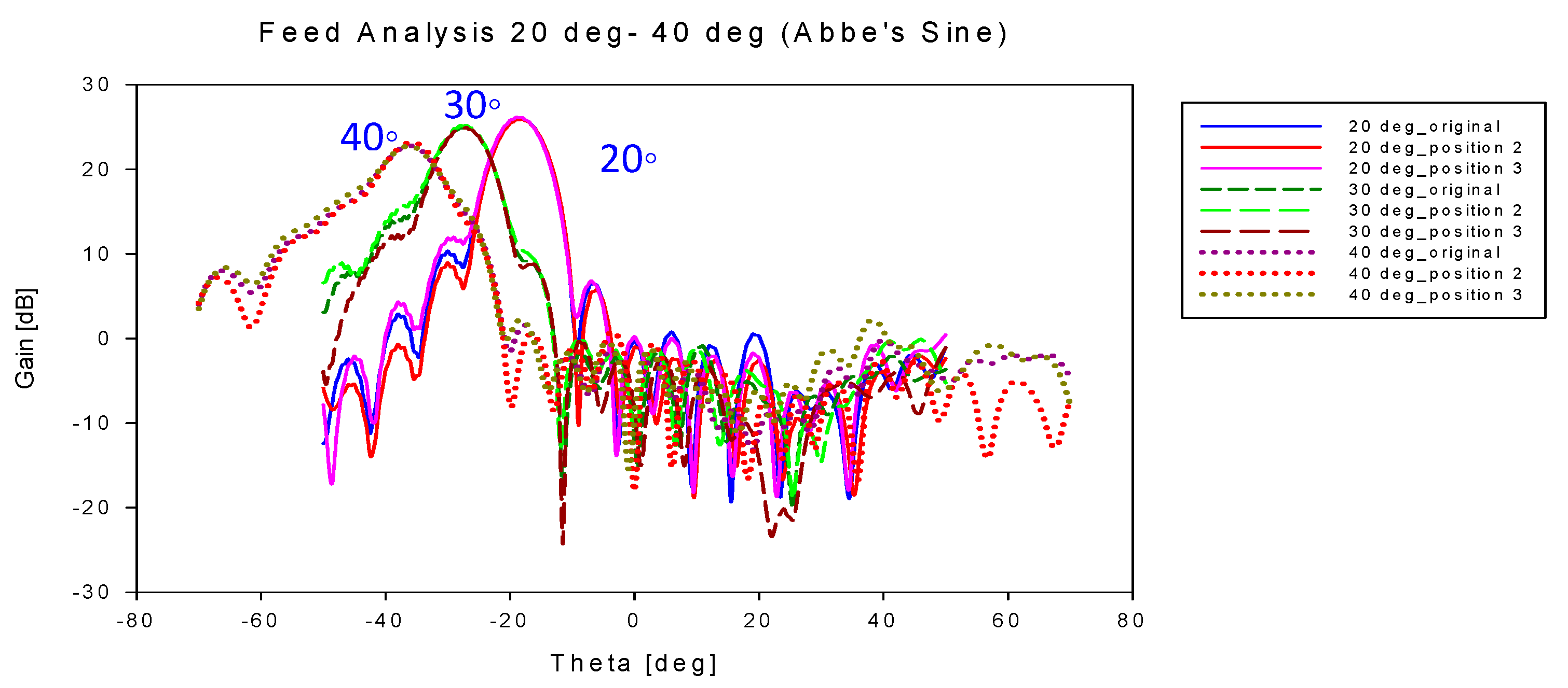
Figure 27.
Antenna gain for all feed position for Abbe’s sine lens.
Figure 27.
Antenna gain for all feed position for Abbe’s sine lens.
Table 1.
Antenna parameters.
Table 1.
Antenna parameters.
| Parameter | Description |
|---|
| Refractive index |
| Feed pattern |
| Aperture Distribution |
| Angle from feed to the lens edge |
Table 2.
Lens parameters.
Table 2.
Lens parameters.
| Parameters | Value |
|---|
| Focal length (mm) | 46.56 |
| (°) | 55 |
| (°) | −24 |
| |
| C | 7 |
| d | 20 |
| Diameter (mm) | 100 |
Table 3.
Calculated n-value.
Table 3.
Calculated n-value.
| Ray in | i (°)
| r (°)
| | Ray out | i (°)
| r (°)
| |
|---|
| 1 | 32 | 19 | 1.62 | 1 | 0.2 | 0.3 | 1.49 |
| 2 | 31 | 19 | 1.58 | 2 | 0.7 | 1.0 | 1.42 |
| 3 | 32 | 20 | 1.54 | 3 | 1.0 | 1.5 | 1.49 |
| 4 | 30 | 20 | 1.46 | 4 | 1.5 | 2.0 | 1.33 |
Table 4.
Lens parameters.
Table 4.
Lens parameters.
| Parameters | Value |
|---|
| fe (mm) | 56.62 |
| (°) | 55 |
| (°) | −24 |
| |
| C | 7 |
| d | 15 |
| Diameter (mm) | 100 |
Table 5.
Calculated -value.
Table 5.
Calculated -value.
| Ray in | i (°)
| r (°)
| | Ray out | i (°)
| r (°)
| |
|---|
| 1 | 28 | 21 | 1.31 | 1 | 0.8 | 1 | 1.25 |
| 2 | 27 | 19 | 1.39 | 2 | 1.6 | 2 | 1.25 |
| 3 | 25 | 17 | 1.45 | 3 | 2 | 3 | 1.50 |
| 4 | 24 | 15 | 1.57 | 4 | 3 | 4 | 1.33 |
Table 6.
Simulation parameters using High Frequency Structure Simulator (HFSS).
Table 6.
Simulation parameters using High Frequency Structure Simulator (HFSS).
| Parameters | Description/Value |
|---|
| Boundary Condition | Radiation Boundary |
| Refractive index, | −1.4142 () |
| Permittivity, | −2 |
| Permeability, | −1 |
Table 7.
Lens structure simulation result.
Table 7.
Lens structure simulation result.
| | Theoretical | Simulation |
|---|
| Gain (dB) | 29.35 | 27.55 |
| (°) | 8.01 | 7.81 |
| (dB) | 0 | −1.80 |
| η (%) | 100 | 66 |
Table 8.
Simulation results of multibeam.
Table 8.
Simulation results of multibeam.
| (°)
| Gain (dB) | (°)
|
|---|
| 0 | 27.55 | 7.81 |
| 10 | 27.14 | 7.72 |
| 20 | 26.50 | 8.31 |
| 30 | 25.18 | 8.97 |
| 40 | 23.09 | 9.06 |
Table 9.
Simulation results.
Table 9.
Simulation results.
| | Theoretical | Simulation |
|---|
| Gain (dB) | 29.35 | 27.48 |
| (°) | 8.01 | 7.64 |
| (dB) | 0 | −1.87 |
| η (%) | 100 | 65 |
Table 10.
Simulation results of different feed positions.
Table 10.
Simulation results of different feed positions.
| (°)
| Gain (dB) | (°)
|
|---|
| 0 | 27.48 | 7.64 |
| 10 | 27.19 | 7.37 |
| 20 | 26.73 | 8.08 |
| 30 | 25.54 | 8.43 |
| 40 | 22.92 | 9.43 |
Table 11.
Performance for all positions at 20°, 30° and 40° scanning angle.
Table 11.
Performance for all positions at 20°, 30° and 40° scanning angle.
| θ | | Focal Length (mm) | Gain (dB) | Beam Width (◦) | SLL (dB) | Shift Angle (◦) |
|---|
| Position | Energy | Abbe | Energy | Abbe | Energy | Abbe | Energy | Abbe | Energy | Abbe |
|---|
| 20 | Original | 46.56 | 56.62 | 26.50 | 26.73 | 8.31 | 8.08 | −17.15 | −17.95 | −18 | −18 |
| Position 2 | 48.68 | 58.74 | 26.12 | 26.55 | 8.36 | 7.95 | −16.63 | −17.93 | −17 | −18 |
| Position 3 | 44.44 | 54.50 | 26.93 | 26.66 | 7.99 | 8.08 | −16.39 | −15.93 | −17 | −18 |
| 30 | Original | 46.56 | 56.62 | 25.18 | 25.54 | 8.97 | 8.43 | −11.65 | −11.37 | −25 | −27 |
| Position 2 | 48.68 | 58.74 | 24.92 | 25.25 | 8.95 | 8.50 | −11.60 | −11.36 | −25 | −27 |
| Position 3 | 44.44 | 54.50 | 25.57 | 25.39 | 9.02 | 8.66 | −12.24 | −11.53 | −26 | −27 |
| 40 | Original | 46.56 | 56.62 | 22.61 | 22.78 | 9.48 | 9.34 | −8.05 | −7.22 | −37 | −36 |
| Position 2 | 48.68 | 58.74 | 22.13 | 23.18 | 9.50 | 9.20 | −5.98 | −7.94 | −37 | −36 |
| Position 3 | 44.44 | 54.50 | 22.92 | 22.73 | 9.61 | 9.41 | −6.68 | −7.81 | −37 | −36 |

 ,
, 


