Lifetime Estimation for Multi-Phase Deteriorating Process with Random Abrupt Jumps †


Abstract
:1. Introduction
2. Motivation and Problem Formulation
3. Lifetime Estimation under the Concept of the FPT
3.1. Lifetime Estimation for Two-Phase Degradation Process without Random Effect
3.2. Lifetime Estimation for Two-Phase Degradation Model with Random Effect
3.3. Lifetime Estimation for Multi-Phase Degradation Model
4. Parameter Identification
4.1. Off-Line Method
4.2. On-Line Updating Method
5. Case Study
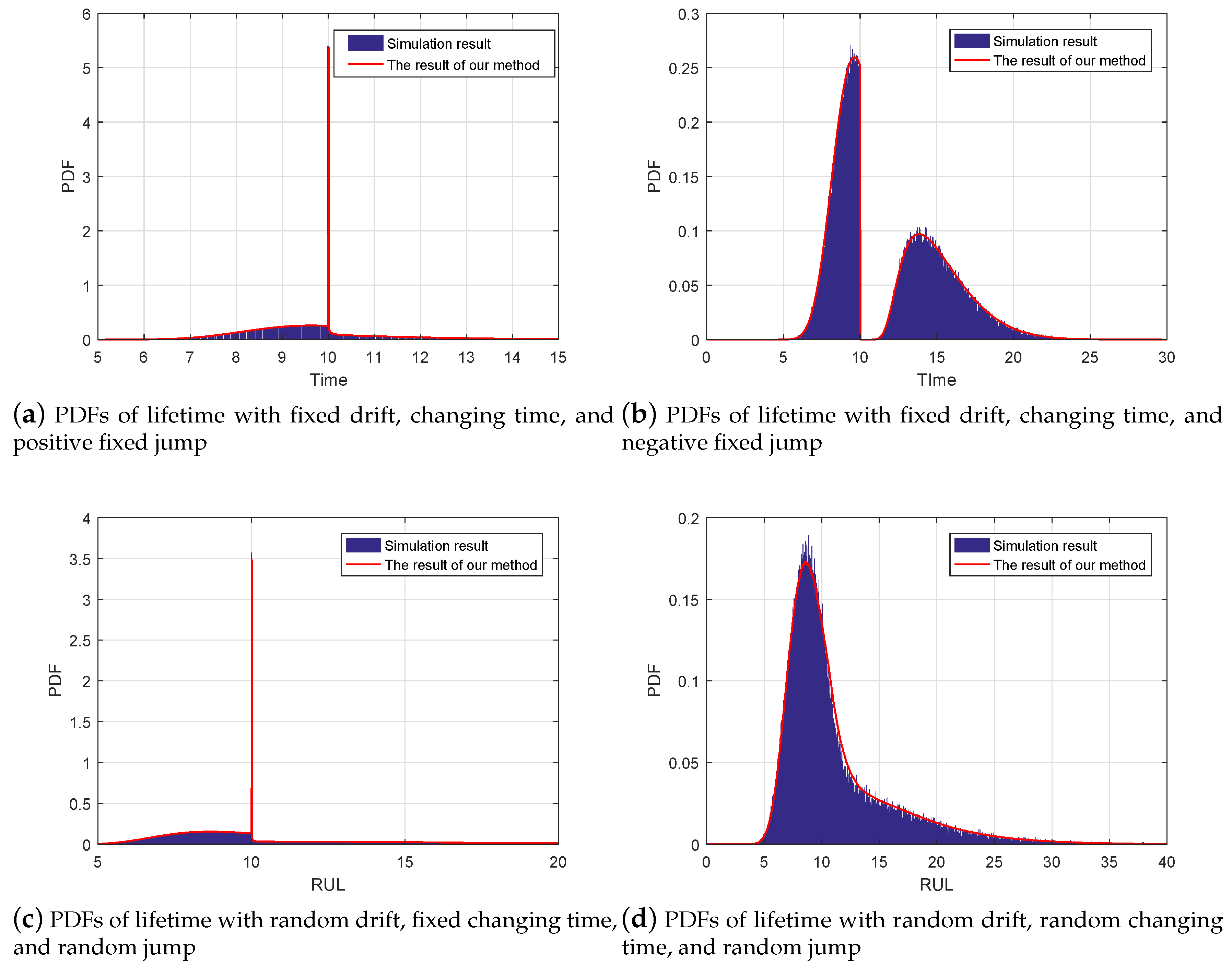
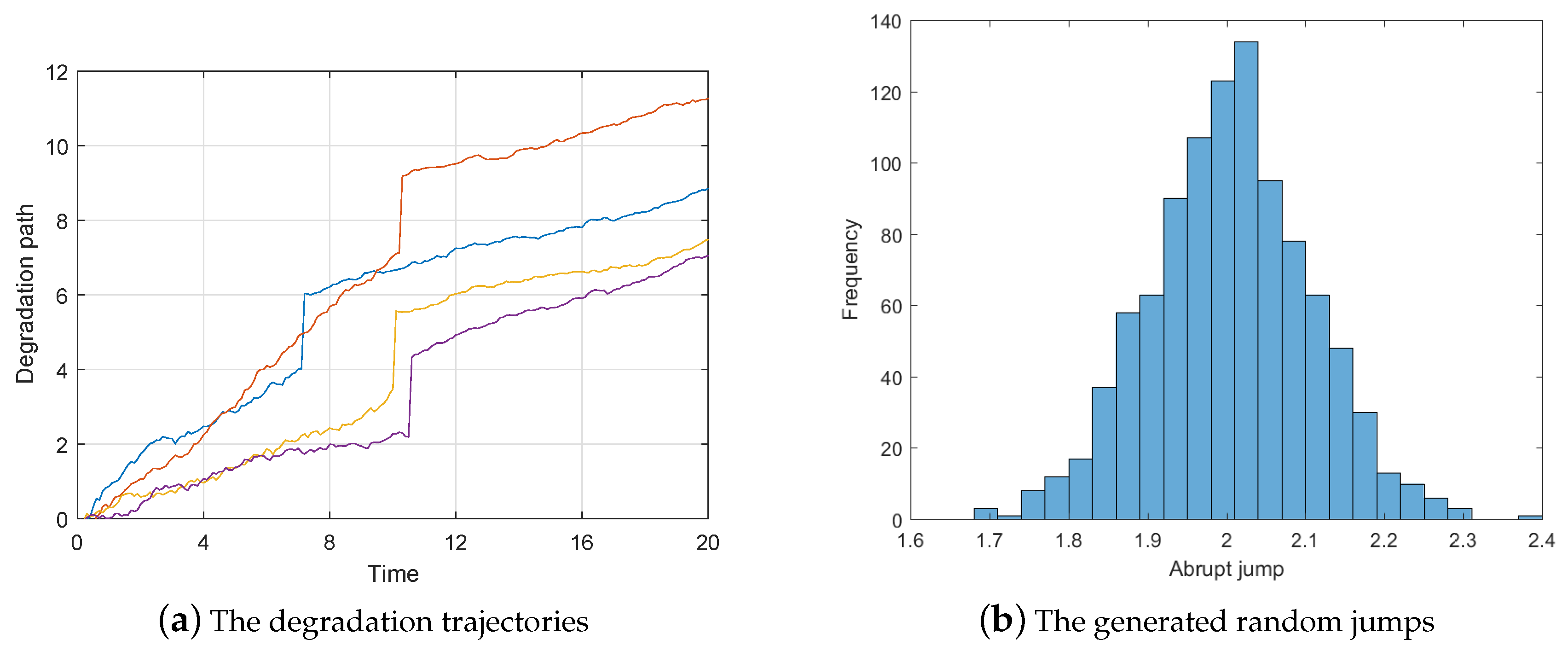
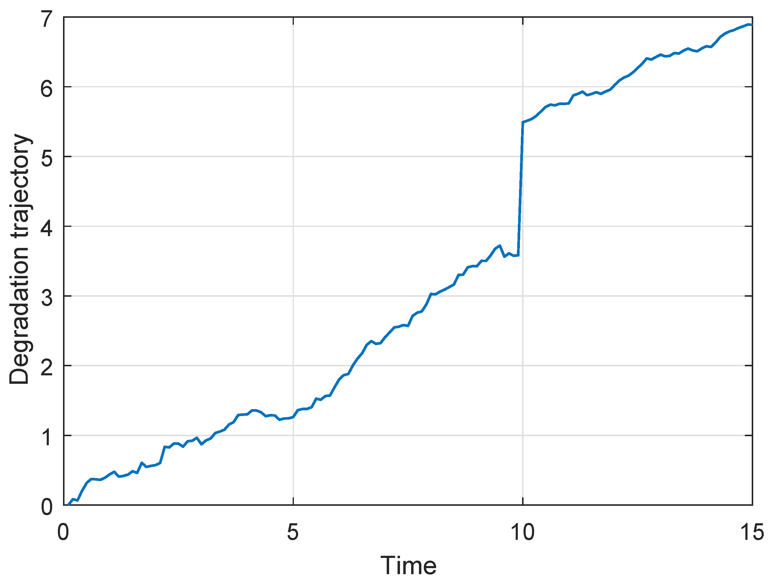
5.1. Numerical Case
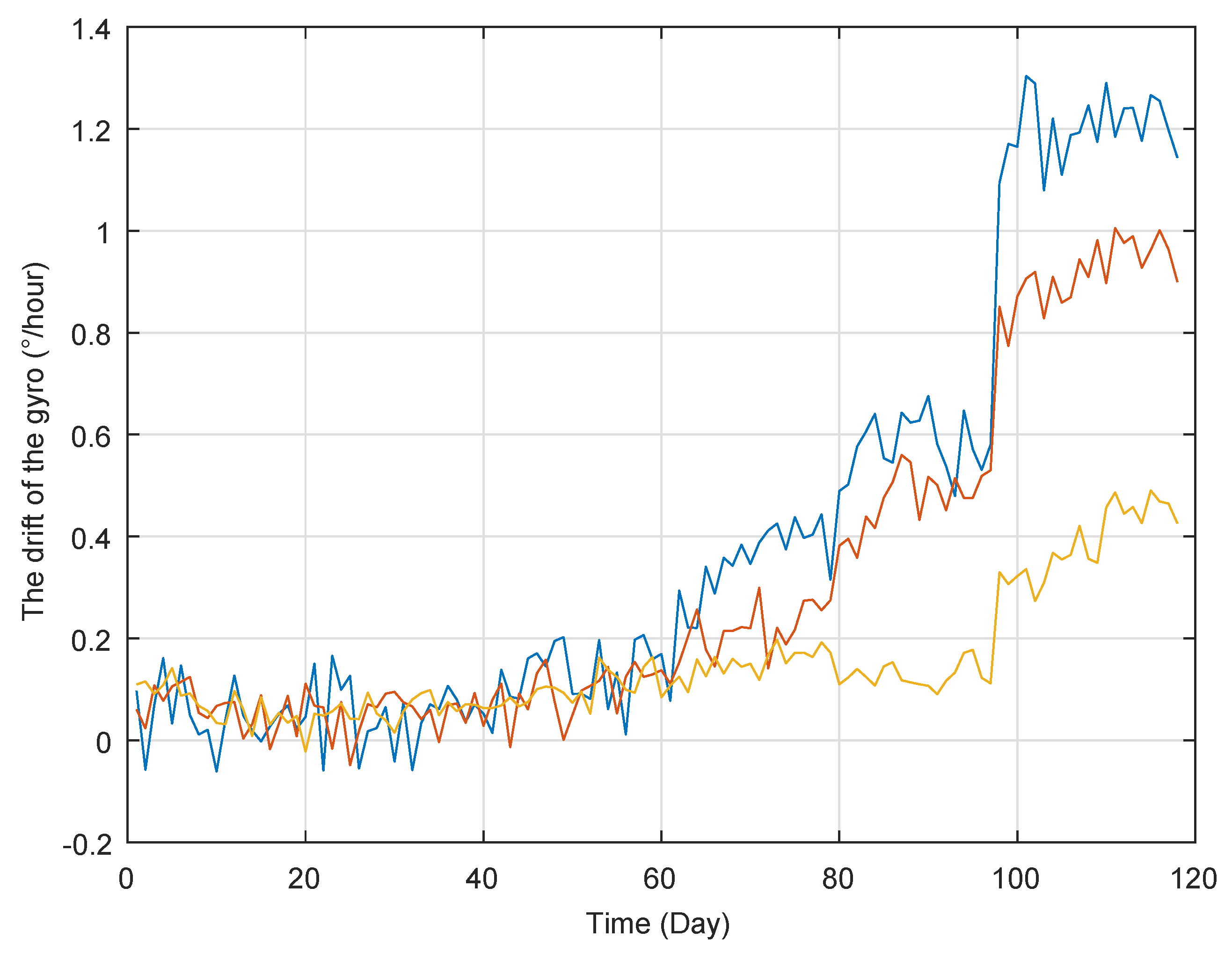
5.2. Practical Case
6. Conclusions
Author Contributions
Funding
Conflicts of Interest
Abbreviations
| RUL | Remaining useful life |
| FPT | First passage time |
| MLE | Maximum Likelihood Estimation |
| EM | Expectation maximum |
| PHM | Prognostic and health management |
| FPT | First passage time |
| Probability density function | |
| CDF | Cumulative distribution function |
| MC | Monte Carlo |
Appendix A
Appendix B
Appendix C
Appendix D
References
- Pecht, M. Prognostics and Health Management of Electronics. In Encyclopedia of Structural Health Monitoring; John Wiley & Sons, Inc.: Hoboken, NJ, USA, 2009. [Google Scholar]
- Vichare, N.M.; Pecht, M.G. Prognostics and health management of electronics. IEEE Trans. Compon. Packag. Technol. 2006, 29, 222–229. [Google Scholar] [CrossRef]
- Si, X.S.; Wang, W.; Hu, C.H.; Zhou, D.H. Remaining useful life estimation—A review on the statistical data driven approaches. Eur. J. Oper. Res. 2011, 213, 1–14. [Google Scholar] [CrossRef]
- Ye, Z.S.; Chen, N.; Shen, Y. A new class of Wiener process models for degradation analysis. Reliab. Eng. Syst. Saf. 2015, 139, 58–67. [Google Scholar] [CrossRef]
- Sun, F.; Liu, L.; Li, X.; Liao, H. Stochastic Modeling and Analysis of Multiple Nonlinear Accelerated Degradation Processes through Information Fusion. Sensors 2016, 16, 1242. [Google Scholar] [CrossRef] [PubMed]
- Jardine, A.K.; Lin, D.; Banjevic, D. A review on machinery diagnostics and prognostics implementing condition-based maintenance. Mech. Syst. Signal Process. 2006, 20, 1483–1510. [Google Scholar] [CrossRef]
- Fernando, S.L.; Paulino Jose, G.N.; Francisco Javier, D.C.J.; Ricardo, M.B.; Victor Manuel, G.S. A hybrid PCA-CART-MARS-based prognostic approach of the remaining useful life for aircraft engines. Sensors 2015, 15, 7062. [Google Scholar]
- Liu, Z.; Mei, W.; Zeng, X.; Yang, C.; Zhou, X. Remaining Useful Life Estimation of Insulated Gate Biploar Transistors (IGBTs) Based on a Novel Volterra k-Nearest Neighbor Optimally Pruned Extreme Learning Machine (VKOPP) Model Using Degradation Data. Sensors 2017, 17, 2524. [Google Scholar] [CrossRef]
- Song, Y.; Liu, D.; Yang, C.; Peng, Y. Data-driven hybrid remaining useful life estimation approach for spacecraft lithium-ion battery. Microelectron. Reliab. 2017, 75, 142–153. [Google Scholar] [CrossRef]
- Si, X.S.; Wang, W.; Hu, C.H.; Chen, M.Y.; Zhou, D.H. A Wiener-process-based degradation model with a recursive filter algorithm for remaining useful life estimation. Mech. Syst. Signal Process. 2013, 35, 219–237. [Google Scholar] [CrossRef]
- Ye, Z.S.; Wang, Y.; Tsui, K.L.; Pecht, M. Degradation Data Analysis Using Wiener Processes with Measurement Errors. IEEE Trans. Reliab. 2013, 62, 772–780. [Google Scholar] [CrossRef]
- Ling, M.H.; Tsui, K.L.; Balakrishnan, N. Accelerated Degradation Analysis for the Quality of a System Based on the Gamma Process. IEEE Trans. Reliab. 2015, 64, 463–472. [Google Scholar] [CrossRef]
- Chen, N.; Ye, Z.S.; Xiang, Y.; Zhang, L. Condition-based maintenance using the inverse Gaussian degradation model. Eur. J. Oper. Res. 2015, 243, 190–199. [Google Scholar] [CrossRef]
- Ye, Z.S.; Chen, N. The Inverse Gaussian Process as a Degradation Model. Technometrics 2014, 56, 302–311. [Google Scholar] [CrossRef]
- Bae, S.J.; Yuan, T.; Ning, S.; Kuo, W. A Bayesian approach to modeling two-phase degradation using change-point regression. Reliab. Eng. Syst. Saf. 2015, 134, 66–74. [Google Scholar] [CrossRef]
- Yan, W.A.; Song, B.W.; Duan, G.L.; Shi, Y.M. Real-time reliability evaluation of two-phase Wiener degradation process. Commun. Stat. Theory Methods 2017, 46, 176–188. [Google Scholar] [CrossRef]
- Wang, X.; Jiang, P.; Guo, B.; Cheng, Z. Real-time Reliability Evaluation for an Individual Product Based on Change-point Gamma and Wiener Process. Qual. Reliab. Eng. Int. 2014, 30, 513–525. [Google Scholar] [CrossRef]
- Park, J.I.; Baek, S.H.; Jeong, M.K.; Bae, S.J. Dual features functional support vector machines for fault detection of rechargeable batteries. IEEE Trans. Syst. Man Cybern. Part C (Appl. Rev.) 2009, 39, 480–485. [Google Scholar] [CrossRef]
- Burgess, W.L. Valve regulated lead acid battery float service life estimation using a Kalman filter. J. Power Sources 2009, 191, 16–21. [Google Scholar] [CrossRef]
- Ng, T.S. An application of the EM algorithm to degradation modeling. IEEE Trans. Reliab. 2008, 57, 2–13. [Google Scholar]
- Bae, S.J.; Kvam, P.H. A change-point analysis for modeling incomplete burn-in for light displays. IIE Trans. 2006, 38, 489–498. [Google Scholar] [CrossRef] [Green Version]
- Wang, Y.; Peng, Y.; Zi, Y.; Jin, X.; Tsui, K.L. A Two-Stage Data-Driven-Based Prognostic Approach for Bearing Degradation Problem. IEEE Trans. Ind. Inform. 2016, 12, 924–932. [Google Scholar] [CrossRef]
- Wang, P.; Tang, Y.; Bae, S.J.; Xu, A. Bayesian Approach for Two-Phase Degradation Data Based on Change-Point Wiener Process With Measurement Errors. IEEE Trans. Reliab. 2018, 67, 688–700. [Google Scholar] [CrossRef]
- Wang, P.; Tang, Y.; Bae, S.J.; He, Y. Bayesian analysis of two-phase degradation data based on change-point Wiener process. Reliab. Eng. Syst. Saf. 2018, 170, 244–256. [Google Scholar] [CrossRef]
- Zhang, J.X.; Hu, C.H.; He, X.; Si, X.S.; Liu, Y.; Zhou, D.H. A Novel Lifetime Estimation Method for Two-Phase Degrading Systems. IEEE Trans. Reliab. 2018, 1–21. [Google Scholar] [CrossRef]
- Kong, D.; Balakrishnan, N.; Cui, L. Two-Phase Degradation Process Model With Abrupt Jump at Change Point Governed by Wiener Process. IEEE Trans. Reliab. 2017, 66, 1345–1360. [Google Scholar] [CrossRef]
- Zhang, J.X.; Hu, C.H.; He, X.; Si, X.S.; Liu, Y.; Zhou, D.H. Lifetime Prognostics for Furnace Wall Degradation with Time-Varying Random Jumps. Reliab. Eng. Syst. Saf. 2017, 167, 338–350. [Google Scholar] [CrossRef]
- Yuan, T.; Bae, S.J.; Zhu, X. A Bayesian approach to degradation-based burn-in optimization for display products exhibiting two-phase degradation patterns. Reliab. Eng. Syst. Saf. 2016, 155, 55–63. [Google Scholar] [CrossRef]
- Chen, N.; Tsui, K.L. Condition monitoring and remaining useful life prediction using degradation signals: Revisited. IIE Trans. 2013, 45, 939–952. [Google Scholar] [CrossRef]
- Si, X.S.; Wang, W.; Chen, M.Y.; Hu, C.H.; Zhou, D.H. A degradation path-dependent approach for remaining useful life estimation with an exact and closed-form solution. Eur. J. Oper. Res. 2013, 226, 53–66. [Google Scholar] [CrossRef]
- Saxena, A.; Celaya, J.; Balaban, E.; Kai, G.; Saha, B.; Saha, S.; Schwabacher, M. Metrics for evaluating performance of prognostic techniques. In Proceedings of the International Conference on Prognostics and Health Management, Denver, CO, USA, 6–9 October 2008; pp. 1–17. [Google Scholar]


| Sample Size | ||||||||||
|---|---|---|---|---|---|---|---|---|---|---|
| n = 5 | ||||||||||
| n = 10 | ||||||||||
| n = 50 | ||||||||||
| True value |
| Algorithm Procedure: | |
|---|---|
| Step 1. | Identify the parameters by the historical data based on the method in Section 4.1. |
| Step 2. | Collect the operating degradation data, and then detect the appearing of the change point if the change time is not known. |
| Step 3. | Update the parameters of the first phase model based on the method in Section 4.2 until the the change point appears. Otherwise, update the parameters of the second phase model. |
| Step 4. | Estimate the RUL online based on the result in Section 3 and Remark 2. |
| Step 5. | Collect latest degradation data and then go to step 2 until degradation reaches the predefined failure threshold. |
© 2019 by the authors. Licensee MDPI, Basel, Switzerland. This article is an open access article distributed under the terms and conditions of the Creative Commons Attribution (CC BY) license (http://creativecommons.org/licenses/by/4.0/).
Share and Cite
Zhang, J.; Si, X.; Du, D.; Hu, C.; Hu, C. Lifetime Estimation for Multi-Phase Deteriorating Process with Random Abrupt Jumps. Sensors 2019, 19, 1472. https://doi.org/10.3390/s19061472
Zhang J, Si X, Du D, Hu C, Hu C. Lifetime Estimation for Multi-Phase Deteriorating Process with Random Abrupt Jumps. Sensors. 2019; 19(6):1472. https://doi.org/10.3390/s19061472
Chicago/Turabian StyleZhang, Jianxun, Xiaosheng Si, Dangbo Du, Chen Hu, and Changhua Hu. 2019. "Lifetime Estimation for Multi-Phase Deteriorating Process with Random Abrupt Jumps" Sensors 19, no. 6: 1472. https://doi.org/10.3390/s19061472