Adversarial Samples on Android Malware Detection Systems for IoT Systems

 ,
,  and
and 
Abstract
:1. Introduction
- We migrated the application of adversarial samples from the image recognition domain to the Android malware detection domain of IoT devices. In this process, simply replacing the model’s training data from a picture to an Android application is not possible. On the one hand, the data of the binary program is not continuous like the image data. On the other hand, random perturbation of the binary program may lead to the crash of the program, so special processing is required for the Android application to ensure the validity of the adversarial samples. We borrowed the processing method of Kathrin Grosse [28], which realized the disturbance to the Android application by adding the request permission code in the file. The difference is that we have made corresponding analysis and restrictions on the types and quantities of permissions that can be added. This method can ensure that the original function of the app is not affected and can be used normally; and the app can be disturbed in the simplest way to achieve the effect of changing the model detection result;
- We introduce the genetic algorithm into the adversarial sample generation method and implement the black-box attack against the machine learning model. Without knowing the internal parameters such as the gradient and structure of the target network, it is only necessary to know the probability of various types of labels output by the model. Compared to Kathrin Grosse’s approach, our approach not only implements black-box attacks, but also has a higher success rate, almost 100%.
2. Related Background
2.1. Neural Network
2.2. Genetic Algorithm
2.3. Adversarial Samples
3. Methodology
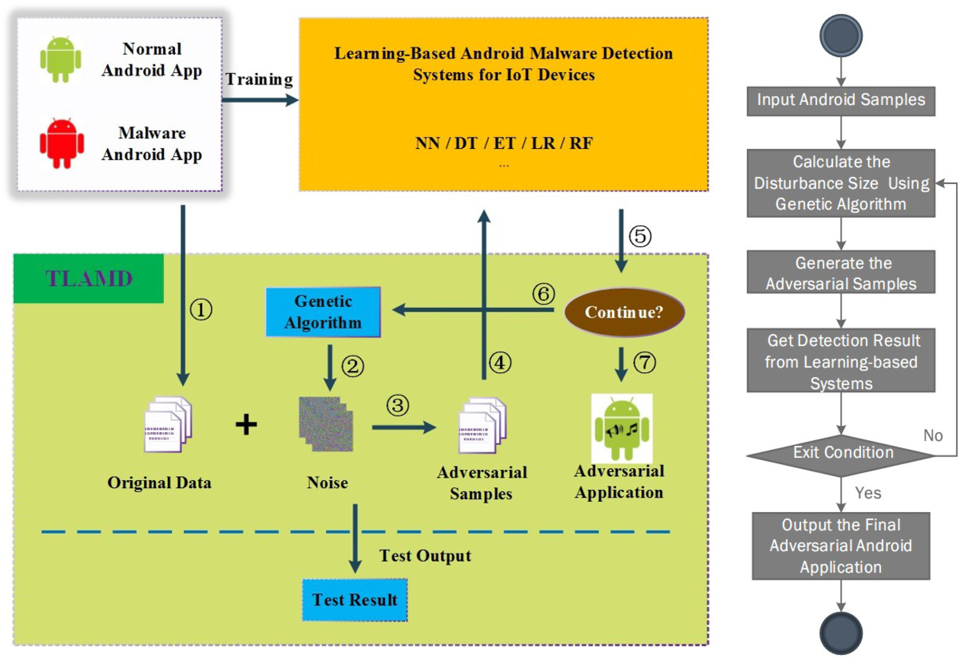
3.1. Framework
3.2. Algorithm
| Algorithm 1 Generating an adversarial sample. |
| Require: Popluation Size for do Compute if then Continue else Output end if end for |
- (1)
- Randomly generate the population . M is the number of individuals, the individual refers to the permission characteristics to be added in the category, and n is the number of permission features in the category. In addition, 1 means to add the corresponding permission; otherwise, 0 means not to add. Our strategy is to only add permissions and not reduce permissions. Therefore, if the original malicious sample has a certain permission feature, the permission cannot be removed, that is, the disturbance is 0.
- (2)
- Determine the fitness function.where and represent the two weights, is the added small disturbance, means that the probability of original malicious sample is still detected as a malware, indicates the number of permission features added.When is much larger than , the sample after the addition of the disturbance must be detected as normal by the detection model to survive, and the individual detected as a malicious sample will be eliminated. The surviving individual must meet the minimum number of added permission features; otherwise, it will also be eliminated. The fitness function defined in this way searches for an optimal solution that can successfully cause the detection model to be misjudged.
- (3)
- Perform mutation operations according to a certain probability to generate new individuals. The mutation refers to adding a disturbance to the corresponding category according to a certain probability, that is, changing the value from 0 to 1, and satisfying the constraint proposed in step (1).
- (4)
- Generate a new generation of the population from the mutation and return to step (2). If the preset number of iterations is reached, the loop is exited.
4. Experiments
4.1. Data Set and Environment
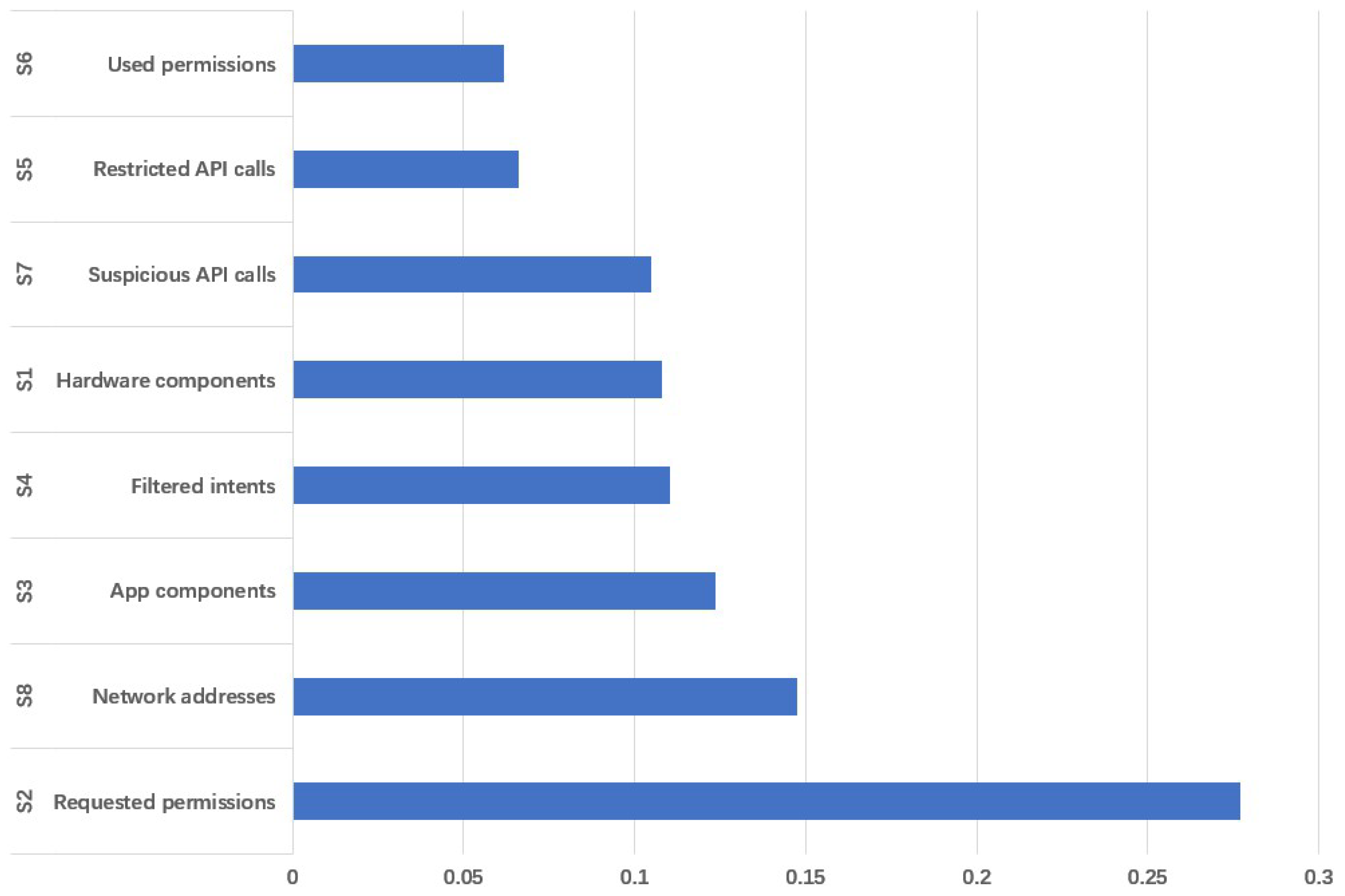
- (S1)
- Hardware components, which are used to set the hardware permissions required by the software.
- (S2)
- Requested permissions, which are granted by the user at the time of installation and allow the application software to access the corresponding resources.
- (S3)
- App components, which include four different types of interfaces: activities, services, content providers and broadcast receivers.
- (S4)
- Filtered intents, which are used for process communication between different components and applications.
- (S5)
- Restricted API (Application Programming Interface) calls, access to a series of key API calls.
- (S6)
- Used permissions, a subset of permissions that are actually used and requested in S5.
- (S7)
- Suspicious API calls, API calls for allowing access to sensitive data and resources.
- (S8)
- Network addresses, the IP addresses accessed by the application, including the hostname and URL.
4.2. Android Malware Detection Model
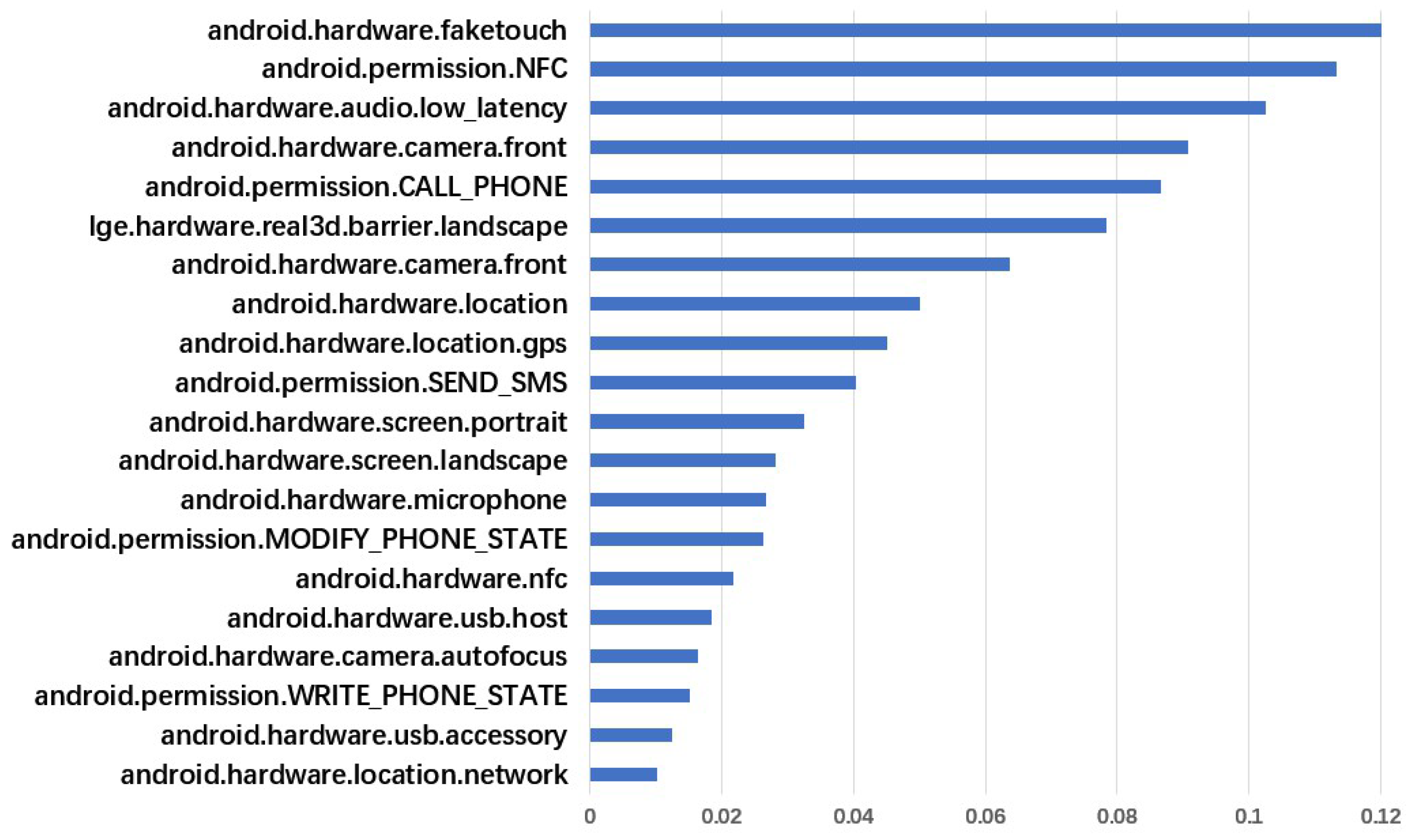
4.2.1. Feature Extraction
- (1)
- Select out of bag (OOB) to calculate the corresponding out-of-bag data deviation for each decision tree.
- (2)
- Add random noise, perturb all samples of OOB, and then calculate the out-of-bag data deviation again.
- (3)
- Define and calculate the importance of the features:where N is the number of forest decision trees.If is greatly increased after adding random noise, the OOB accuracy rate decreases, indicating that this type of feature has a greater impact on the prediction result, that is, the importance is higher.
4.2.2. Training Detection Model
- a.
- Neural Network
- b.
- Logistic Regression
- c.
- Decision Tree
- d.
- Random Forest
- e.
- Extreme Tree
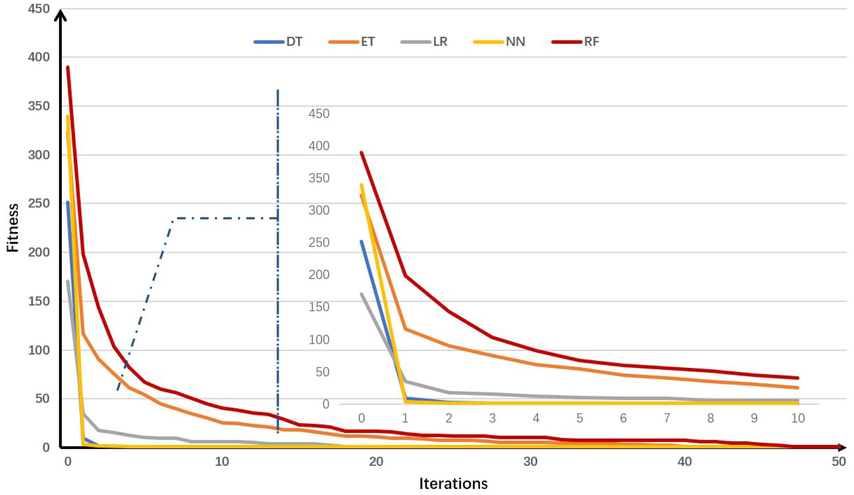
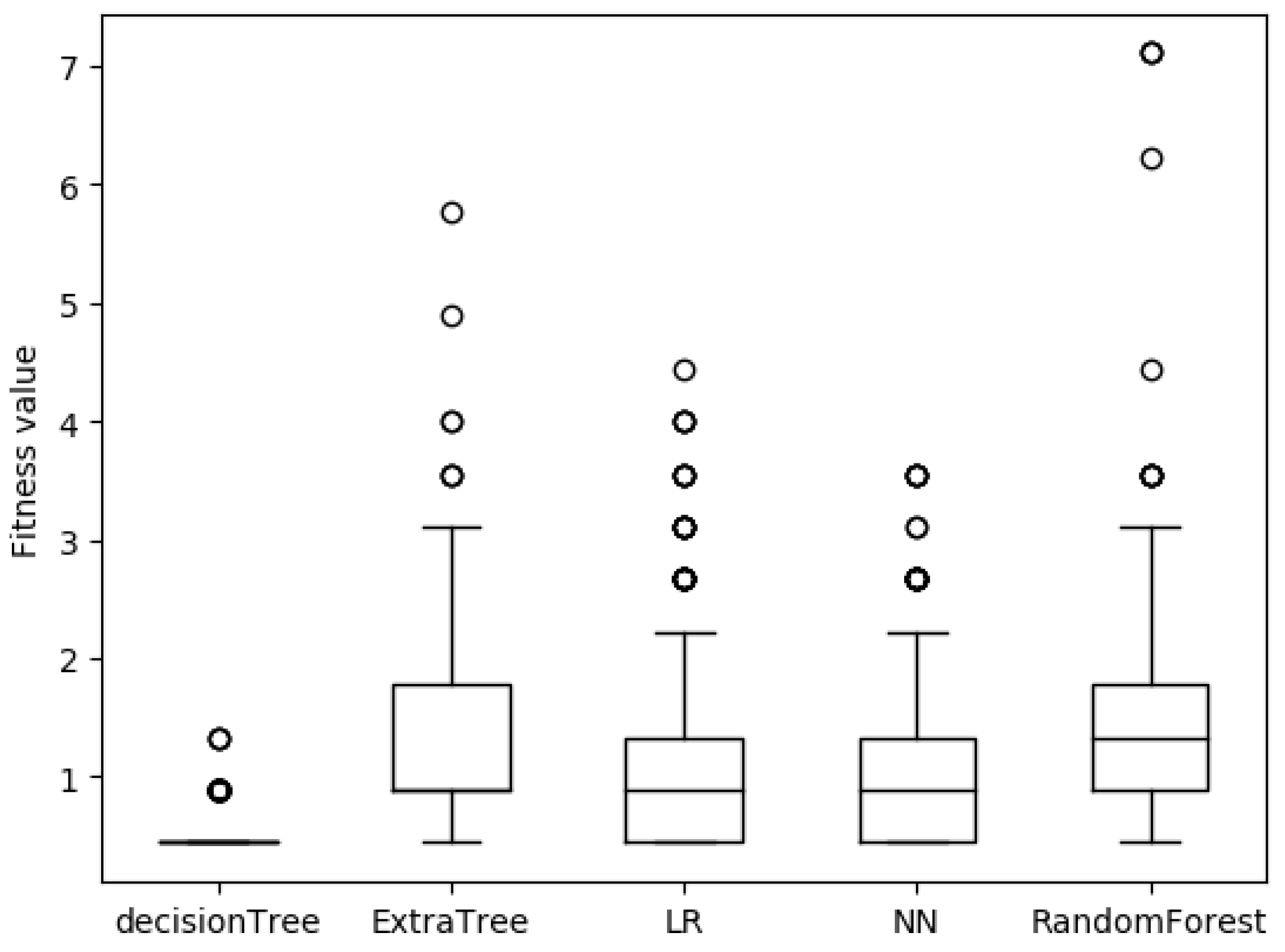
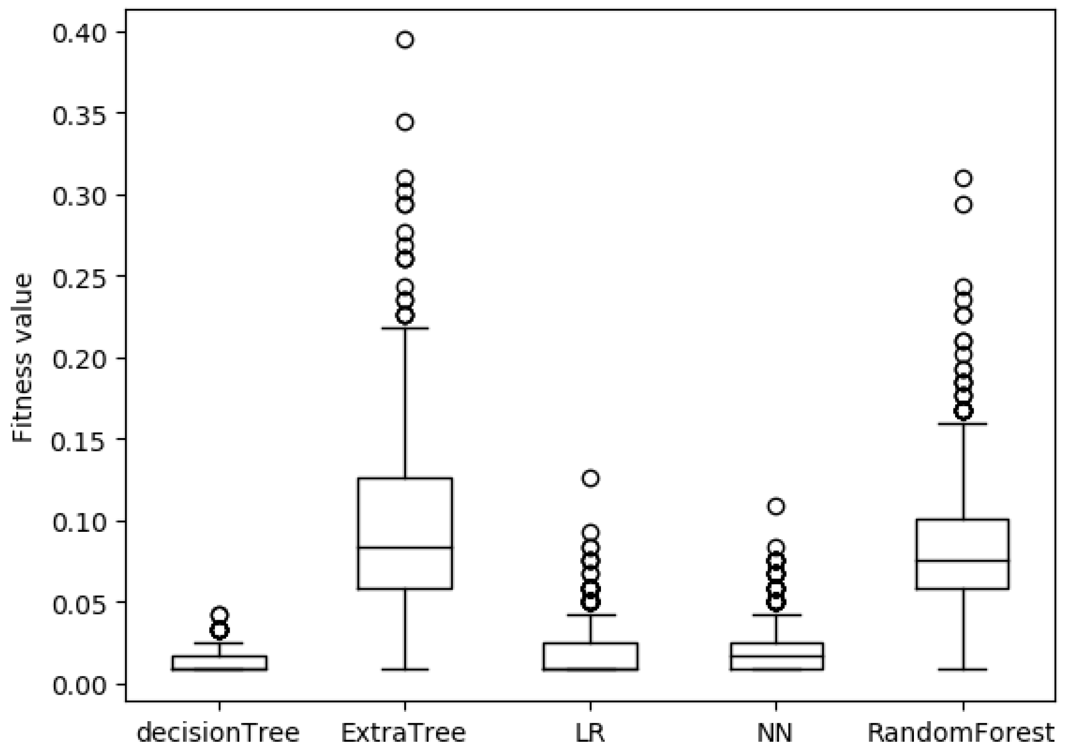
4.3. Simulation Experiments
5. Conclusions
Author Contributions
Funding
Conflicts of Interest
References
- Ham, H.S.; Kim, H.H.; Kim, M.S.; Choi, M.J. Linear SVM-based android malware detection for reliable IoT services. J. Appl. Math. 2014, 2014, 594501. [Google Scholar] [CrossRef]
- McNeil, P.; Shetty, S.; Guntu, D.; Barve, G. SCREDENT: Scalable Real-time Anomalies Detection and Notification of Targeted Malware in Mobile Devices. Procedia Comput. Sci. 2016, 83, 1219–1225. [Google Scholar] [CrossRef] [Green Version]
- Aswini, A.; Vinod, P. Towards the Detection of Android Malware using Ensemble Features. J. Inf. Assur. Secur. 2015, 10, 9–21. [Google Scholar]
- Odusami, M.; Abayomi-Alli, O.; Misra, S.; Shobayo, O.; Damasevicius, R.; Maskeliunas, R. Android Malware Detection: A Survey. In Proceedings of the International Conference on Applied Informatics Applied Informatics, Bogota, Colombia, 1–3 November 2018; Florez, H., Diaz, C., Chavarriaga, J., Eds.; Springer International Publishing: Cham, Switzerland, 2018; pp. 255–266. [Google Scholar]
- Misra, S.; Adewumi, A.; Maskeliūnas, R.; Damaševičius, R.; Cafer, F. Unit Testing in Global Software Development Environment. In Proceedings of the International Conference on Recent Developments in Science, Engineering and Technology, Gurgaon, India, 13–14 October 2017; Springer: Berlin, Germany, 2017; pp. 309–317. [Google Scholar]
- Alhassan, J.; Misra, S.; Umar, A.; Maskeliūnas, R.; Damaševičius, R.; Adewumi, A. A Fuzzy Classifier-Based Penetration Testing for Web Applications. In Proceedings of the International Conference on Information Theoretic Security, Libertad City, Ecuador, 10–12 January 2018; Springer: Berlin, Germany, 2018; pp. 95–104. [Google Scholar] [Green Version]
- Barreno, M.; Nelson, B.; Joseph, A.D.; Tygar, J.D. The security of machine learning. Mach. Learn. 2010, 81, 121–148. [Google Scholar] [CrossRef] [Green Version]
- Wu, L.; Du, X.; Wu, J. Effective defense schemes for phishing attacks on mobile computing platforms. IEEE Trans. Veh. Technol. 2016, 65, 6678–6691. [Google Scholar] [CrossRef]
- Cheng, Y.; Fu, X.; Du, X.; Luo, B.; Guizani, M. A lightweight live memory forensic approach based on hardware virtualization. Inf. Sci. 2017, 379, 23–41. [Google Scholar] [CrossRef]
- Hei, X.; Du, X.; Lin, S.; Lee, I. PIPAC: Patient infusion pattern based access control scheme for wireless insulin pump system. In Proceedings of the 2013 Proceedings IEEE INFOCOM, Turin, Italy, 14–19 April 2013; pp. 3030–3038. [Google Scholar]
- Du, X.; Xiao, Y.; Guizani, M.; Chen, H.H. An effective key management scheme for heterogeneous sensor networks. Ad Hoc Netw. 2007, 5, 24–34. [Google Scholar] [CrossRef]
- Du, X.; Guizani, M.; Xiao, Y.; Chen, H.H. Transactions papers a routing-driven Elliptic Curve Cryptography based key management scheme for Heterogeneous Sensor Networks. IEEE Trans. Wirel. Commun. 2009, 8, 1223–1229. [Google Scholar] [CrossRef]
- Du, X.; Chen, H.H. Security in wireless sensor networks. IEEE Trans. Wirel. Commun. 2008, 15, 60–66. [Google Scholar]
- Biggio, B.; Fumera, G.; Roli, F.; Didaci, L. Poisoning adaptive biometric systems. In Proceedings of the Joint IAPR International Workshops on Statistical Techniques in Pattern Recognition (SPR) and Structural and Syntactic Pattern Recognition (SSPR), Hiroshima, Japan, 7–9 Novembe 2012; Springer: Berlin, Germany, 2012; pp. 417–425. [Google Scholar]
- Biggio, B.; Didaci, L.; Fumera, G.; Roli, F. Poisoning attacks to compromise face templates. In Proceedings of the 2013 International Conference on Biometrics (ICB), Madrid, Spain, 4–7 June 2013; pp. 1–7. [Google Scholar]
- Biggio, B.; Fumera, G.; Roli, F. Pattern recognition systems under attack: Design issues and research challenges. Int. J. Pattern Recognit. Artif. Intell. 2014, 28, 1460002. [Google Scholar] [CrossRef]
- Zhu, X. Super-class Discriminant Analysis: A novel solution for heteroscedasticity. Pattern Recognit. Lett. 2013, 34, 545–551. [Google Scholar] [CrossRef]
- Biggio, B.; Nelson, B.; Laskov, P. Poisoning attacks against support vector machines. arXiv, 2012; arXiv:1206.6389. [Google Scholar]
- Yang, C.; Wu, Q.; Li, H.; Chen, Y. Generative poisoning attack method against neural networks. arXiv, 2017; arXiv:1703.01340. [Google Scholar]
- Szegedy, C.; Zaremba, W.; Sutskever, I.; Bruna, J.; Erhan, D.; Goodfellow, I.; Fergus, R. Intriguing properties of neural networks. arXiv, 2013; arXiv:1312.6199. [Google Scholar]
- Carlini, N.; Wagner, D. Towards evaluating the robustness of neural networks. In Proceedings of the 2017 IEEE Symposium on Security and Privacy (SP), San Jose, CA, USA, 22–26 May 2017; pp. 39–57. [Google Scholar]
- Moosavi-Dezfooli, S.M.; Fawzi, A.; Fawzi, O.; Frossard, P. Universal adversarial perturbations. arXiv, 2017; arXiv:1610.08401. [Google Scholar]
- Warde-Farley, D.; Goodfellow, I. 11 adversarial perturbations of deep neural networks. In Perturbations, Optimization, and Statistics; MIT Press: Cambridge, MA, USA, 2016; p. 311. [Google Scholar]
- Papernot, N.; McDaniel, P.; Jha, S.; Fredrikson, M.; Celik, Z.B.; Swami, A. The limitations of deep learning in adversarial settings. In Proceedings of the 2016 IEEE European Symposium on Security and Privacy (EuroS&P), Saarbrücken, Germany, 21–24 March 2016; pp. 372–387. [Google Scholar]
- Chen, S.; Xue, M.; Fan, L.; Hao, S.; Xu, L.; Zhu, H.; Li, B. Automated poisoning attacks and defenses in malware detection systems: An adversarial machine learning approach. Comput. Secur. 2018, 73, 326–344. [Google Scholar] [CrossRef] [Green Version]
- Chen, L.; Hou, S.; Ye, Y.; Xu, S. Droideye: Fortifying security of learning-based classifier against adversarial android malware attacks. In Proceedings of the 2018 IEEE/ACM International Conference on Advances in Social Networks Analysis and Mining (ASONAM), Barcelona, Spain, 28–31 August 2018; pp. 782–789. [Google Scholar]
- Al-Dujaili, A.; Huang, A.; Hemberg, E.; O’Reilly, U.M. Adversarial deep learning for robust detection of binary encoded malware. In Proceedings of the 2018 IEEE Security and Privacy Workshops (SPW), San Francisco, CA, USA, 24 May 2018; pp. 76–82. [Google Scholar]
- Grosse, K.; Papernot, N.; Manoharan, P.; Backes, M.; McDaniel, P. Adversarial examples for malware detection. In Proceedings of the European Symposium on Research in Computer Security, Oslo, Norway, 11–15 September 2017; pp. 62–79. [Google Scholar]
- Maas, A.L.; Hannun, A.Y.; Ng, A.Y. Rectifier nonlinearities improve neural network acoustic models. In Proceedings of the 30th International Conference on Machine Learning, Atlanta, GA, USA, 16–21 June 2013; Volume 30, p. 3. [Google Scholar]
- Mishkin, D.; Matas, J. All you need is a good init. arXiv, 2015; arXiv:1511.06422. [Google Scholar]
- Chen, Z.; Lin, T.; Tang, N.; Xia, X. A parallel genetic algorithm based feature selection and parameter optimization for support vector machine. Sci. Progr. 2016, 2016, 2739621. [Google Scholar] [CrossRef]
- Phan, A.V.; Le Nguyen, M.; Bui, L.T. Feature weighting and SVM parameters optimization based on genetic algorithms for classification problems. Appl. Intell. 2017, 46, 455–469. [Google Scholar] [CrossRef]
- Alejandre, F.V.; Cortés, N.C.; Anaya, E.A. Feature selection to detect botnets using machine learning algorithms. In Proceedings of the 2017 International Conference on Electronics, Communications and Computers (CONIELECOMP), Cholula, Mexico, 22–24 February 2017; pp. 1–7. [Google Scholar]
- Papernot, N.; McDaniel, P.; Goodfellow, I.; Jha, S.; Celik, Z.B.; Swami, A. Practical black-box attacks against machine learning. In Proceedings of the 2017 ACM on Asia Conference on Computer and Communications Security, Abu Dhabi, UAE, 2–6 April 2017; pp. 506–519. [Google Scholar]
- Papernot, N.; McDaniel, P.; Goodfellow, I.; Jha, S.; Celik, Z.B.; Swami, A. Practical black-box attacks against deep learning systems using adversarial examples. arXiv, 2016; arXiv:1602.02697. [Google Scholar]
- Papernot, N.; McDaniel, P.; Goodfellow, I. Transferability in machine learning: from phenomena to black-box attacks using adversarial samples. arXiv, 2016; arXiv:1605.07277. [Google Scholar]
- Narodytska, N.; Kasiviswanathan, S.P. Simple Black-Box Adversarial Attacks on Deep Neural Networks. In Proceedings of the CVPR Workshops, Honolulu, HI, USA, 21–26 July 2017; pp. 1310–1318. [Google Scholar]
- Papernot, N.; McDaniel, P.; Wu, X.; Jha, S.; Swami, A. Distillation as a defense to adversarial perturbations against deep neural networks. In Proceedings of the 2016 IEEE Symposium on Security and Privacy (SP), San Jose, CA, USA, 23–25 May 2016; pp. 582–597. [Google Scholar]
- Arp, D.; Spreitzenbarth, M.; Hubner, M.; Gascon, H.; Rieck, K.; Siemens, C. DREBIN: Effective and Explainable Detection of Android Malware in Your Pocket. In Proceedings of the Network and Distributed System Security Symposium (NDSS), San Diego, CA, USA, 23–26 February 2014; Volume 14, pp. 23–26. [Google Scholar]
- Spreitzenbarth, M.; Freiling, F.; Echtler, F.; Schreck, T.; Hoffmann, J. Mobile-sandbox: having a deeper look into android applications. In Proceedings of the 28th Annual ACM Symposium on Applied Computing, Coimbra, Portugal, 18–22 March 2013; pp. 1808–1815. [Google Scholar]


| CPU | Inter(R) Core(TM) i5-7400 CPU @ 3.00GHz |
|---|---|
| Memery | 8 GB |
| Video Card | Inter(R) HD Graphics 630 |
| Operating System | Windows 10 |
| Programming Language | Python 3.6 |
| Development Platform | Jupyter Notebook |
| Dependence | Tensorflow, Keras, numpy etc. |
| Class | Name | Numbers | Rate (/Total) |
|---|---|---|---|
| S1 | Hardware Components | 72 | 0.013% |
| S2 | Requested Permissions | 3812 | 0.704% |
| S3 | App Components | 218,951 | 40.488% |
| S4 | Filtered Intents | 6379 | 1.178% |
| S5 | Restricted API Calls | 733 | 0.136% |
| S6 | Used Permissions | 70 | 0.013% |
| S7 | Suspicious API Calls | 315 | 0.058% |
| S8 | Network Address | 310,447 | 57.4% |
| Models | TP | FP | FN | TN | Accuracy | Precision | Recall |
|---|---|---|---|---|---|---|---|
| NN (Neural Network) | 40770 | 0 | 74 | 1726 | 99.83% | 1 | 95.95% |
| LR (Logistic Regression) | 40770 | 0 | 234 | 1566 | 99.45% | 1 | 96.32% |
| DT (Decision Tree) | 40770 | 0 | 60 | 1740 | 99.86% | 1 | 95.91% |
| RF (Random Forest) | 40770 | 0 | 32 | 1768 | 99.92% | 1 | 95.85% |
| ET (Extreme Tree) | 40770 | 0 | 16 | 1784 | 99.96% | 1 | 95.81% |
| Features | S1: Hardware Components | S2: Requested Permissions |
|---|---|---|
| Initialize Probability | 1% | 0.01% |
| Mutation Probability | 30% | 0.5% |
| Iterations | 50 | 50 |
| Population | 150 | 150 |
| Attacked Samples | 1000 | 1000 |
| Model | Category | Success Rate | Average of |
|---|---|---|---|
| NN | S1 | 1 | 2.25 |
| S2 | 1 | 2.33 | |
| LR | S1 | 0.998 | 2.66 |
| S2 | 0.995 | 1.94 | |
| DT | S1 | 0.896 | 1.05 |
| S2 | 0.992 | 1.68 | |
| RF | S1 | 0.866 | 2.89 |
| S2 | 0.995 | 9.54 | |
| ET | S1 | 0.833 | 2.81 |
| S2 | 0.945 | 9.36 |
© 2019 by the authors. Licensee MDPI, Basel, Switzerland. This article is an open access article distributed under the terms and conditions of the Creative Commons Attribution (CC BY) license (http://creativecommons.org/licenses/by/4.0/).
Share and Cite
Liu, X.; Du, X.; Zhang, X.; Zhu, Q.; Wang, H.; Guizani, M. Adversarial Samples on Android Malware Detection Systems for IoT Systems. Sensors 2019, 19, 974. https://doi.org/10.3390/s19040974
Liu X, Du X, Zhang X, Zhu Q, Wang H, Guizani M. Adversarial Samples on Android Malware Detection Systems for IoT Systems. Sensors. 2019; 19(4):974. https://doi.org/10.3390/s19040974
Chicago/Turabian StyleLiu, Xiaolei, Xiaojiang Du, Xiaosong Zhang, Qingxin Zhu, Hao Wang, and Mohsen Guizani. 2019. "Adversarial Samples on Android Malware Detection Systems for IoT Systems" Sensors 19, no. 4: 974. https://doi.org/10.3390/s19040974