Body Dimension Measurements of Qinchuan Cattle with Transfer Learning from LiDAR Sensing

 ,
,
Abstract
:1. Introduction
1.1. Livestock Body Measuring with LiDAR
1.2. Applications of Deep Learning
1.3. Main Purposes
- A new processing fusion for the 3D PCD of cattle is proposed. The original cattle PCD sensed by the LiDAR sensor was filtered by conditional, statistical, and voxel filtering, and then segmented by methods of Euclidean and RANSAC clustering. After the normalization of PCD and orientation correction of body shape, the fast point feature histogram (FPFH) was extracted to retrieve the body silhouettes and local surfaces.
- A 3D classification framework of the target cattle body based on transfer learning is presented. The PyTorch framework of the Kd-network was trained by the ShapeNet PCD dataset. The prior knowledge, the case-based transfer learning of the TrAdaBoost algorithm retrained by the collected cattle silhouettes, was applied to transfer the 3D silhouette of the point cloud and to classify the target cattle body point cloud. The PCD of the cattle body was normalized to extract the candidate surfaces of the feature points, and with extraction of FPFH, the feature points of the cattle body dimensions could be recognized.
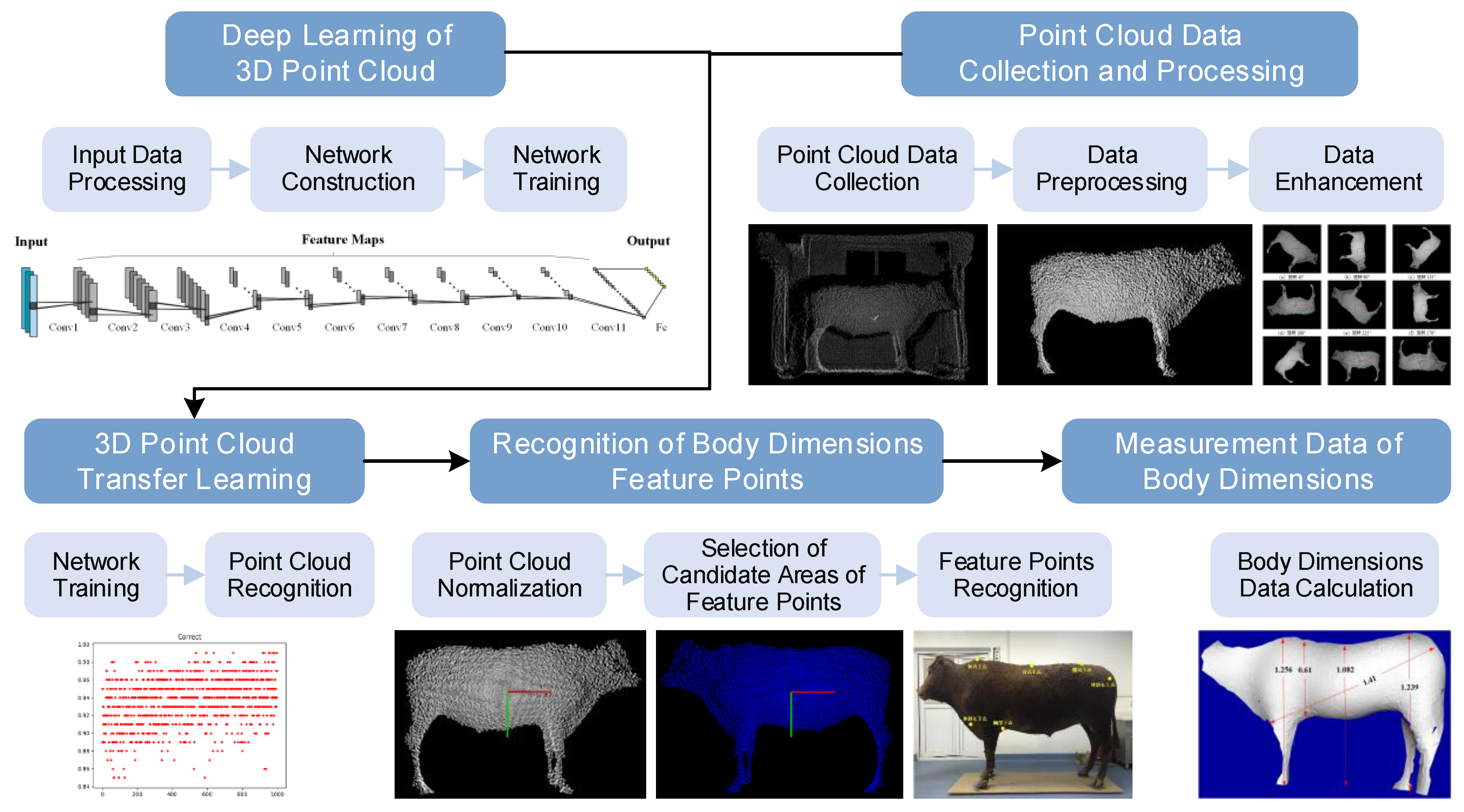
2. Materials and Methods
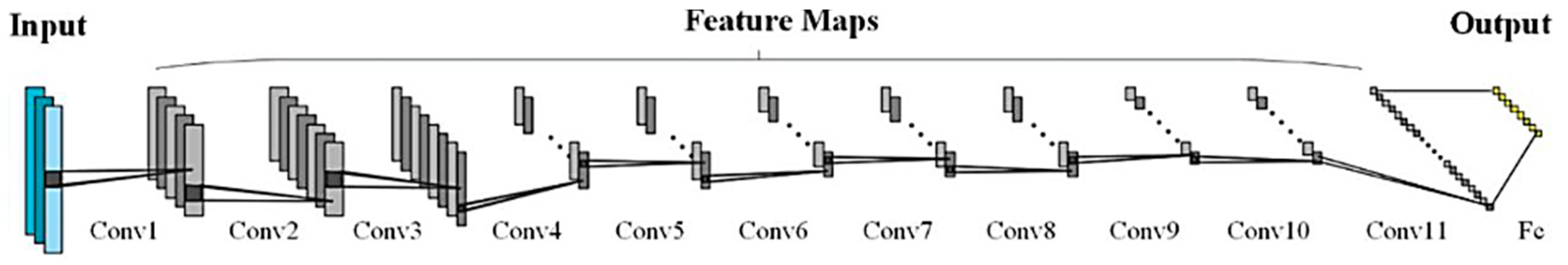
2.1. D Point Cloud Deep Learning Network
2.2. Cattle Body Point Cloud Recognition Based on Transfer Learning
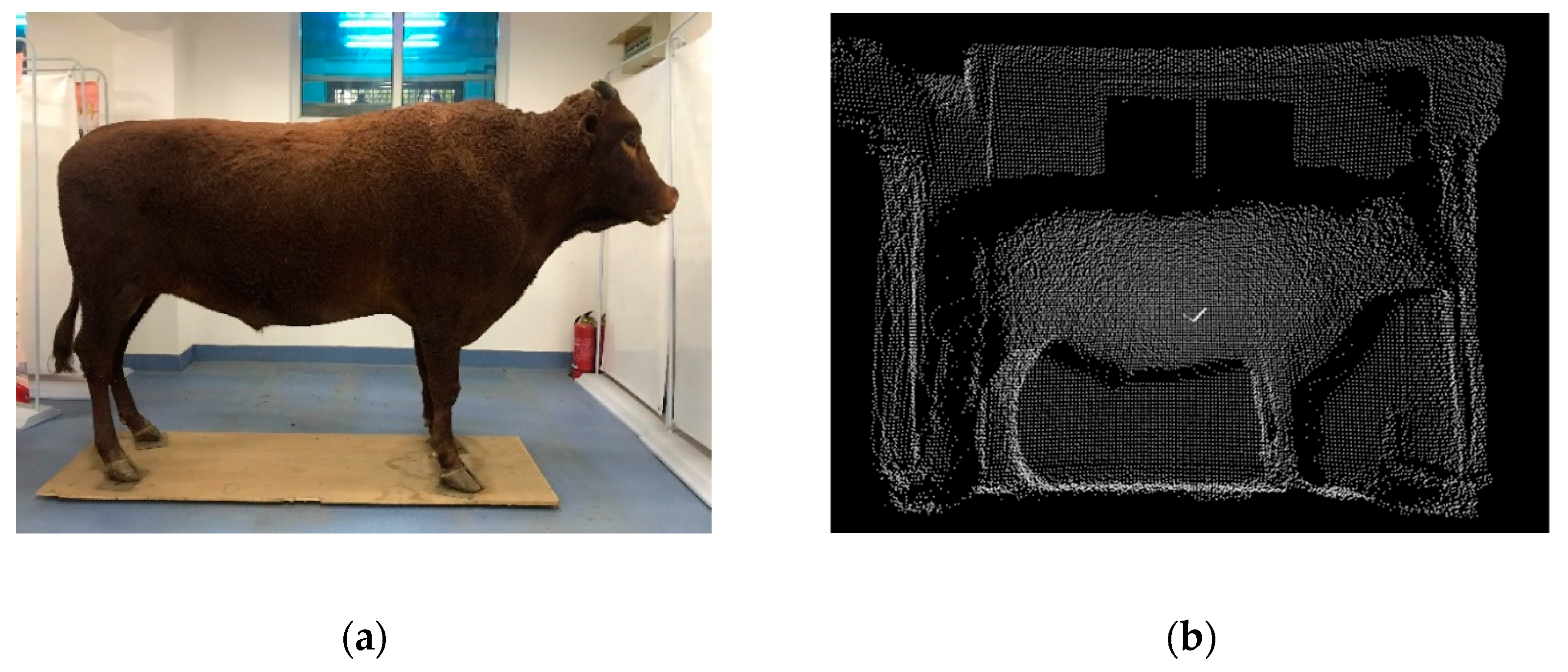
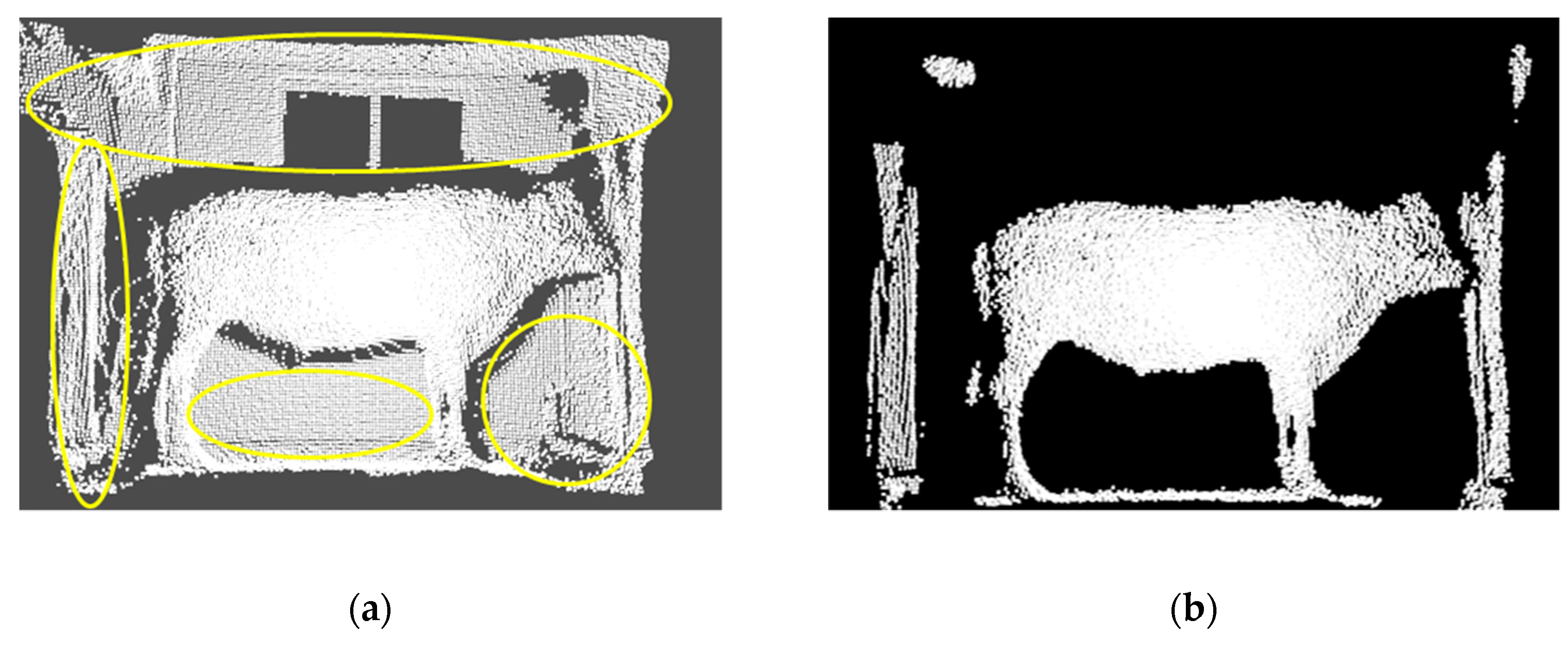
2.2.1. Data Acquisition and Preprocessing
2.2.2. Design of Transfer Learning Network Structure
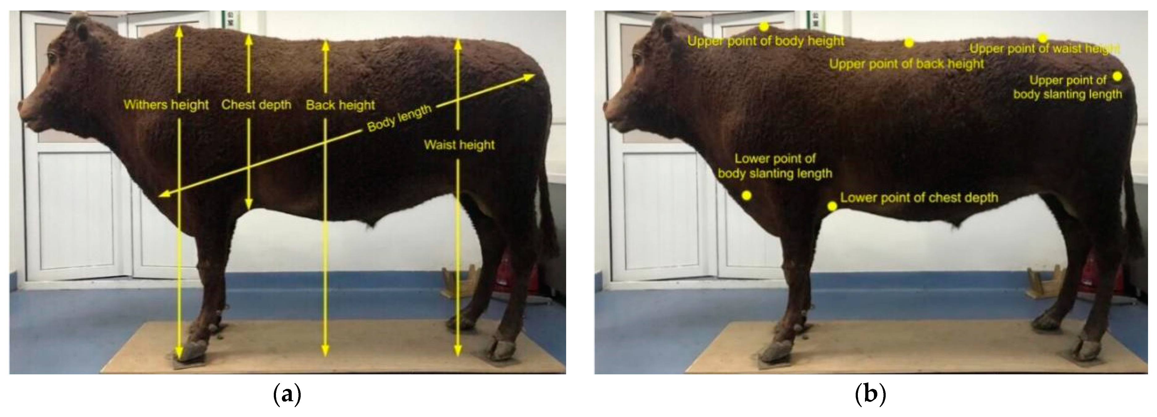
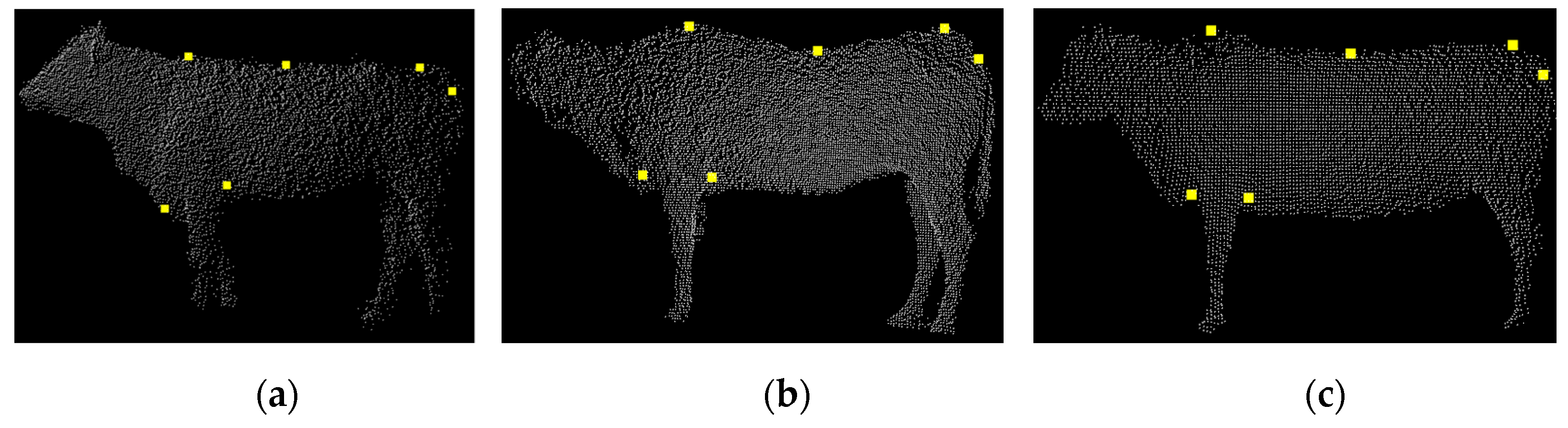
2.3. Recognition of Feature Points of Live Qinchuan Cattle Body
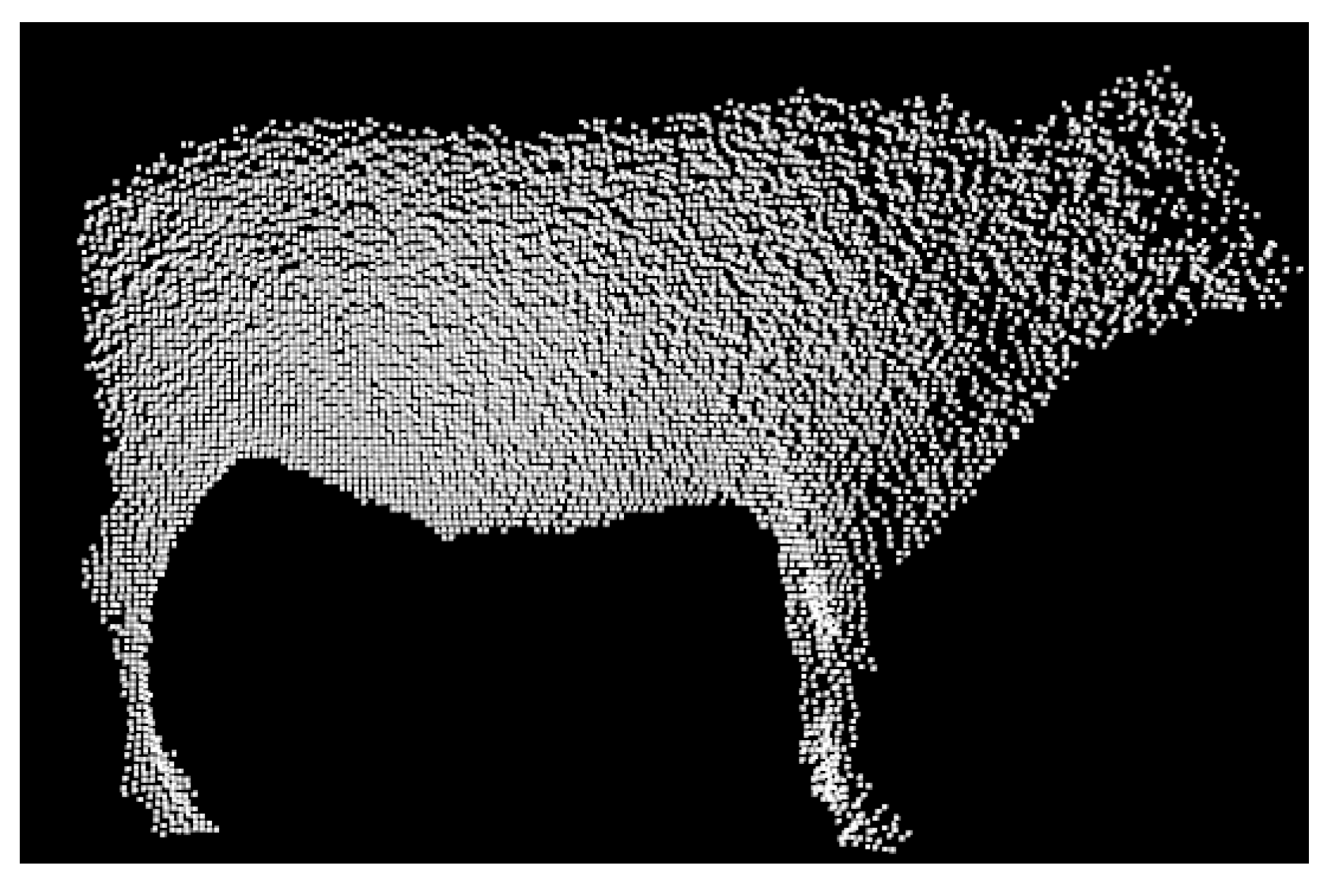
2.3.1. Normalization of Cattle Body Point Cloud
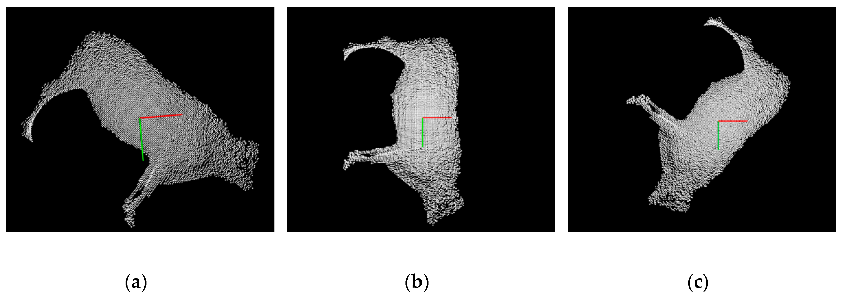
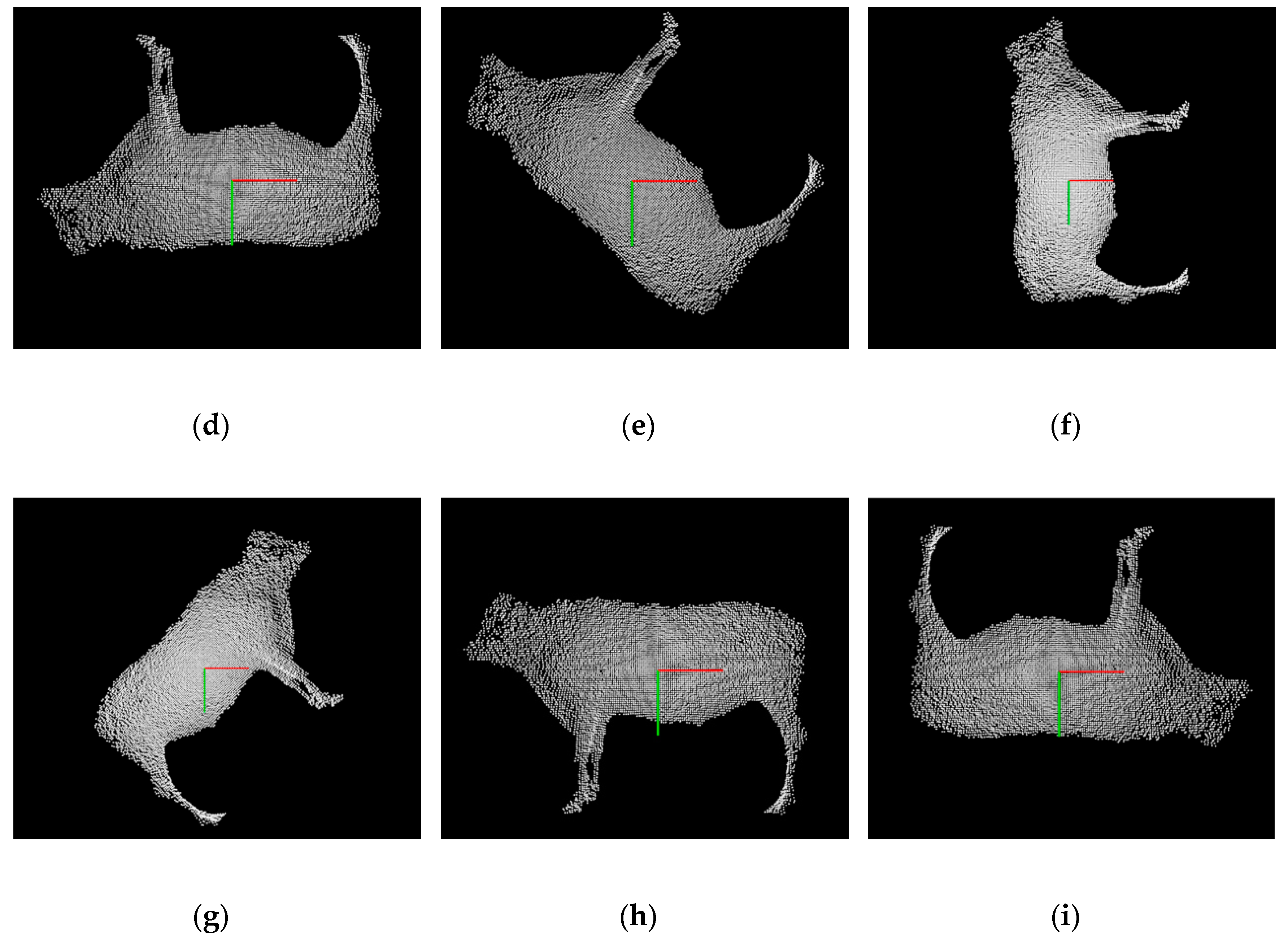
2.3.2. Extraction of the Candidate Areas of Feature Points
2.3.3. Feature Point Recognition
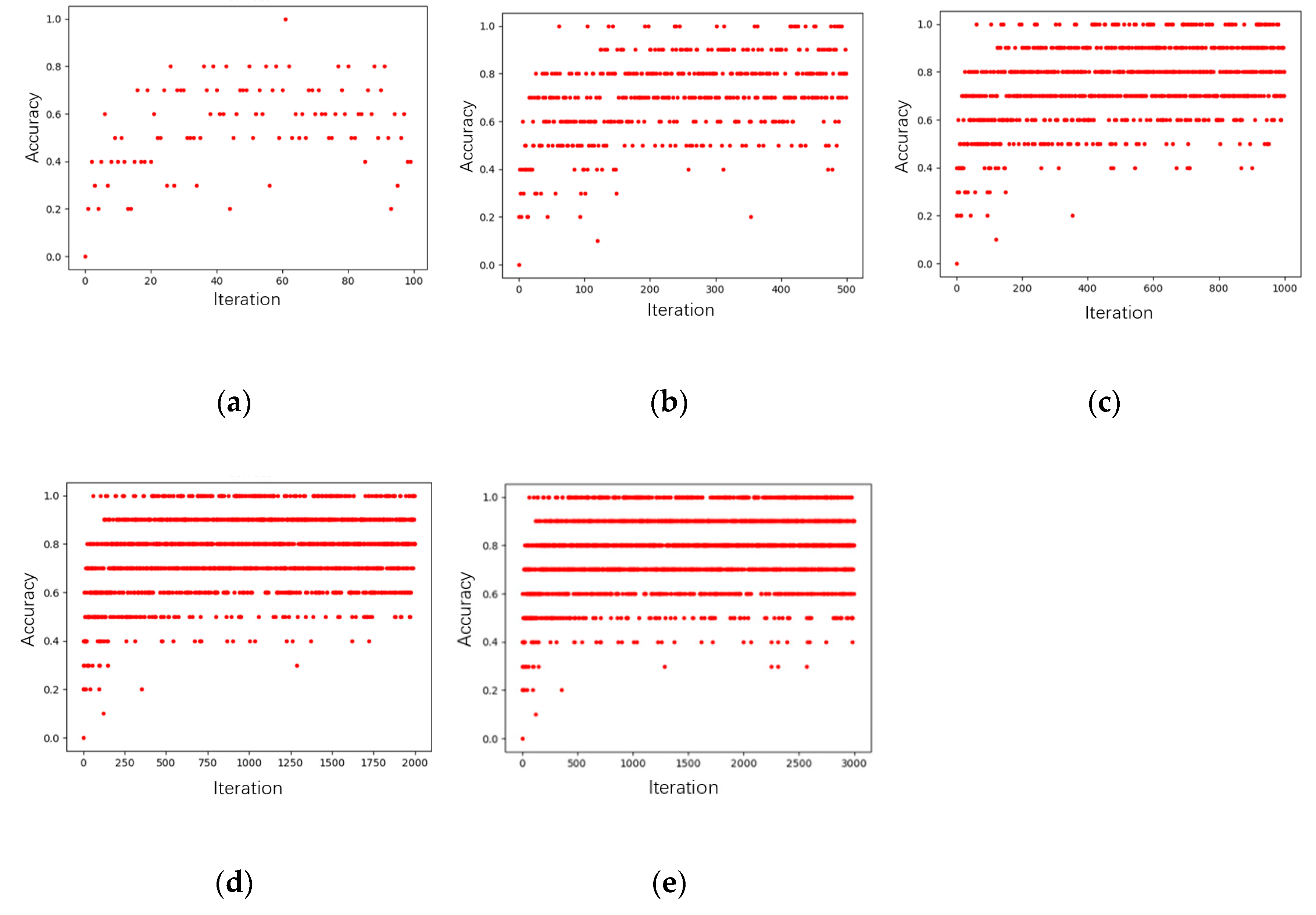
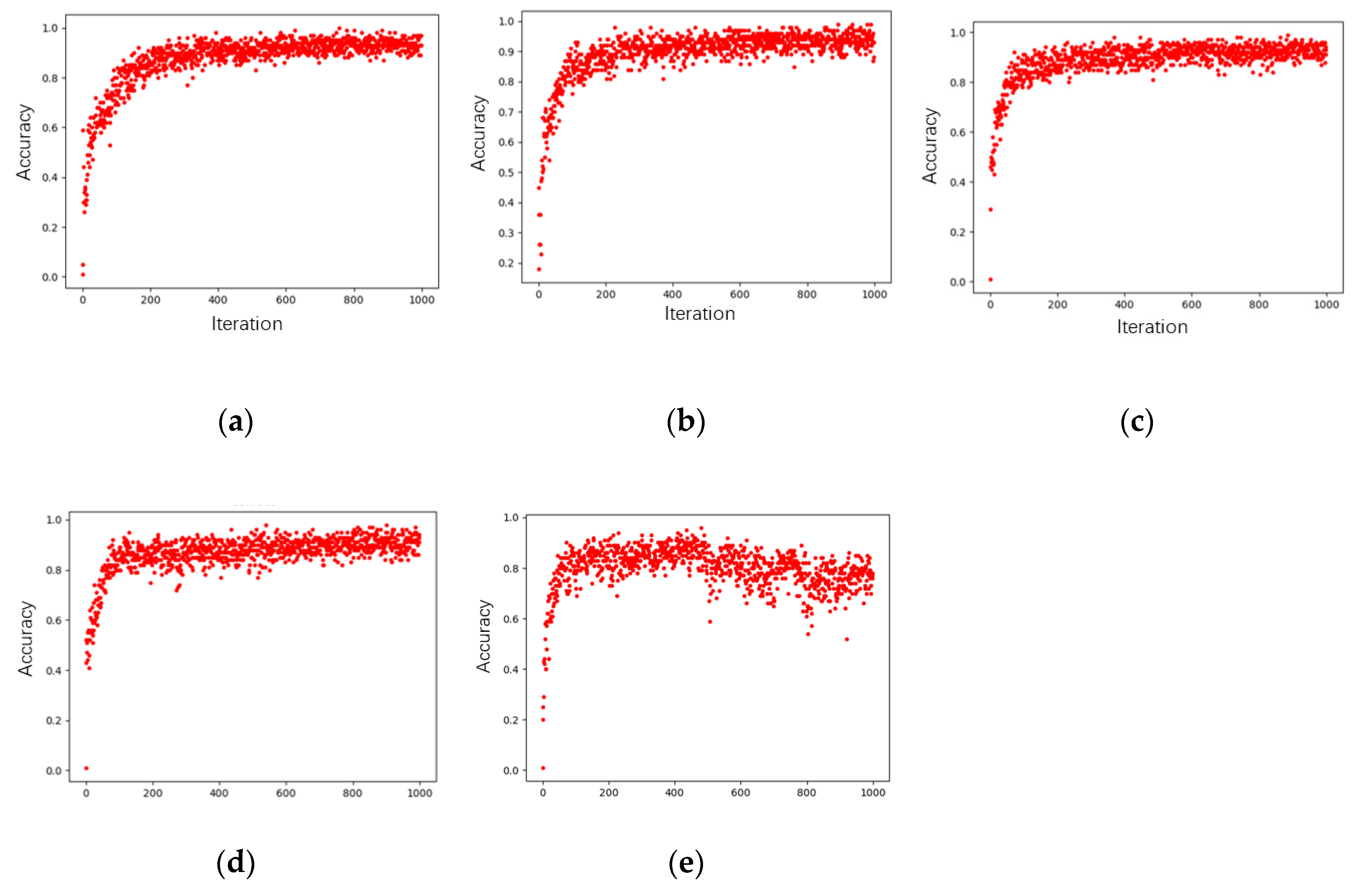
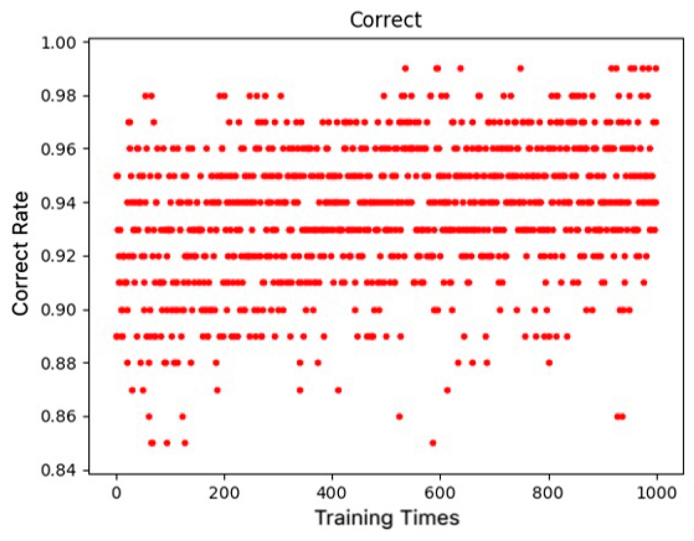
3. Results
4. Discussion
5. Conclusions
Author Contributions
Funding
Acknowledgments
Conflicts of Interest
References
- Salau, J.; Haas, J.H.; Junge, W.; Bauer, U.; Harms, J.; Bieletzki, S. Feasibility of automated body trait determination using the SR4K time-of-flight camera in cow barns. SpringerPlus 2014, 3, 225. [Google Scholar] [CrossRef]
- Pezzuolo, A.; Guarino, M.; Sartori, L.; Marinello, F. A Feasibility study on the use of a structured light depth-camera for three-dimensional body measurements of dairy cows in free-stall barns. Sensors 2018, 18, 673. [Google Scholar] [CrossRef] [PubMed]
- Guo, H.; Ma, X.; Ma, Q.; Wang, K.; Su, W.; Zhu, D. LSSA_CAU: An interactive 3d point clouds analysis software for body measurement of livestock with similar forms of cows or pigs. Comput. Electron. Agric. 2017, 138, 60–68. [Google Scholar] [CrossRef]
- Pezzuolo, A.; Guarino, M.; Sartori, L.; González, L.A.; Marinello, F. On-barn pig weight estimation based on body measurements by a Kinect v1 depth camera. Comput. Electron. Agric. 2018, 148, 29–36. [Google Scholar] [CrossRef]
- Enevoldsen, C.; Kristensen, T. Estimation of body weight from body size measurements and body condition scores in dairy cows. J. Dairy Sci. 1997, 80, 1988–1995. [Google Scholar] [CrossRef]
- Brandl, N.; Jorgensen, E. Determination of live weight of pigs from dimensions measured using image analysis. Comput. Electron. Agric. 1996, 15, 57–72. [Google Scholar] [CrossRef]
- Wilson, L.L.; Egan, C.L.; Terosky, T.L. Body measurements and body weights of special-fed Holstein veal calves. J. Dairy Sci. 1997, 80, 3077–3082. [Google Scholar] [CrossRef]
- Communod, R.; Guida, S.; Vigo, D.; Beretti, V.; Munari, E.; Colombani, C.; Superchi, P.; Sabbioni, A. Body measures and milk production, milk fat globules granulometry and milk fatty acid content in Cabannina cattle breed. Ital. J. Anim. Sci. 2013, 12, 107–115. [Google Scholar] [CrossRef]
- Huang, L.; Li, S.; Zhu, A.; Fan, X.; Zhang, C.; Wang, H. Non-contact body measurement for qinchuan cattle with LiDAR sensor. Sensors 2018, 18, 3014. [Google Scholar] [CrossRef]
- McPhee, M.J.; Walmsley, B.J.; Skinner, B.; Littler, B.; Siddell, J.P.; Cafe, L.M.; Wilkins, J.F.; Oddy, V.H.; Alempijevic, A. Live animal assessments of rump fat and muscle score in Angus cows and steers using 3-dimensional imaging. J. Anim. Sci. 2017, 95, 1847–1857. [Google Scholar] [CrossRef]
- Rizaldy, A.; Persello, C.; Gevaert, C.; Elberink, S.O.; Vosselman, G. Ground and Multi-Class Classification of Airborne Laser Scanner Point Clouds Using Fully Convolutional Networks. Remote Sens. 2018, 10, 1723. [Google Scholar] [CrossRef]
- He, X.; Wang, A.; Ghamisi, P.; Li, G.; Chen, Y. LiDAR Data Classification Using Spatial Transformation and CNN. IEEE Geosci. Remote Sens. Lett. 2018, 16, 125–129. [Google Scholar] [CrossRef]
- Maltezos, E.; Doulamis, A.; Doulamis, N.; Ioannidis, C. Building Extraction From LiDAR Data Applying Deep Convolutional Neural Networks. IEEE Geosci. Remote Sens. Lett. 2018, 16, 155–159. [Google Scholar] [CrossRef]
- Edson, C.; Wing, M.G. Airborne Light Detection and Ranging (LiDAR) for Individual Tree Stem Location, Height, and Biomass Measurements. Remote Sens. 2011, 3, 2494–2528. [Google Scholar] [CrossRef]
- Maki, N.; Nakamura, S.; Takano, S.; Okada, Y. 3D Model Generation of Cattle Using Multiple Depth-Maps for ICT Agriculture. In Proceedings of the Conference on Complex, Intelligent, and Software Intensive Systems, Matsue, Japan, 4–6 July 2018. [Google Scholar]
- Kawasue, K.; Win, K.D.; Yoshida, K.; Tokunaga, T. Black cattle body shape and temperature measurement using thermography and KINECT sensor. Artif. Life Robot. 2017, 22, 1–7. [Google Scholar] [CrossRef]
- Fernandes, A.F.A.; Dorea, J.R.R.; Fitzgerald, R.; Herring, W.; Rosa, G.J.M. A novel automated system to acquire biometric and morphological measurements and predict body weight of pigs via 3D computer vision. J. Anim. Sci. 2019, 97, 496–508. [Google Scholar] [CrossRef]
- Menesatti, P.; Costa, C.; Antonucci, F.; Steri, R.; Pallottino, F.; Catillo, G. A low-cost stereovision system to estimate size and weight of live sheep. Comput. Electron. Agric. 2014, 103, 33–38. [Google Scholar] [CrossRef]
- Wang, K.; Guo, H.; Ma, Q.; Su, W.; Chen, L.; Zhu, D. A portable and automatic Xtion-based measurement system for pig body size. Comput. Electron. Agric. 2018, 148, 291–298. [Google Scholar] [CrossRef]
- Jun, K.; Kim, S.J.; Ji, H.W. Estimating pig weights from images without constraint on posture and illumination. Comput. Electron. Agric. 2018, 153, 169–176. [Google Scholar] [CrossRef]
- Azzaro, G.; Caccamo, M.; Ferguson, J.D.; Battiato, S.; Farinella, G.M.; Guarnera, G.C.; Puglisi, G.; Petriglieri, R.; Licitra, G. Objective estimation of body condition score by modeling cow body shape from digital images. J. Dairy Sci. 2011, 94, 2126–2137. [Google Scholar] [CrossRef]
- Zhou, Z.; Wang, Y.; Wu, Q.M.J.; Yang, C.; Sun, X. Effective and Efficient Global Context Verification for Image Copy Detection. IEEE Trans. Inf. Forensics Secur. 2017, 12, 48–63. [Google Scholar] [CrossRef]
- Omid-Zohoor, A.; Young, C.; Ta, D.; Murmann, B. Toward Always-On Mobile Object Detection: Energy Versus Performance Tradeoffs for Embedded HOG Feature Extraction. IEEE Trans. Circuits Syst. Video Technol. 2018, 28, 1102–1115. [Google Scholar] [CrossRef]
- Zhou, L.; Li, Q.; Huo, G.; Zhou, Y. Image Classification Using Biomimetic Pattern Recognition with Convolutional Neural Networks Features. Comput. Intell. Neurosci. 2017, 2017, 3792805. [Google Scholar] [CrossRef] [PubMed]
- Litjens, G.; Kooi, T.; Bejnordi, B.E.; Setio, A.A.A.; Ciompi, F.; Ghafoorian, M.; van der Laak, J.A.W.M.; van Ginneken, B.; Sanchez, C.I. A survey on deep learning in medical image analysis. Med. Image Anal. 2017, 42, 60–88. [Google Scholar] [CrossRef] [PubMed]
- Wu, Z.; Song, S.; Khosla, A.; Yu, F.; Zhang, L.; Tang, X.; Xiao, J.; Wu, Z.; Song, S.; Khosla, A. 3D ShapeNets: A deep representation for volumetric shapes. In Proceedings of the IEEE Conference on Computer Vision & Pattern Recognition, Boston, MA, USA, 7–12 June 2015. [Google Scholar]
- Guan, H.; Yu, Y.; Ji, Z.; Li, J.; Zhang, Q. Deep learning-based tree classification using mobile LiDAR data. Remote Sens. Lett. 2015, 6, 864–873. [Google Scholar] [CrossRef]
- Nahhas, F.H.; Shafri, H.Z.M.; Sameen, M.I.; Pradhan, B.; Mansor, S. Deep Learning Approach for Building Detection Using LiDAR-Orthophoto Fusion. J. Sens. 2018, 7. [Google Scholar] [CrossRef]
- Jin, S.; Su, Y.; Gao, S.; Wu, F.; Hu, T.; Liu, J.; Li, W.; Wang, D.; Chen, S.; Jiang, Y.; et al. Deep Learning: Individual Maize Segmentation From Terrestrial Lidar Data Using Faster R-CNN and Regional Growth Algorithms. Front. Plant Sci. 2018, 22, 866. [Google Scholar] [CrossRef]
- Charles, R.Q.; Hao, S.; Mo, K.; Guibas, L.J. PointNet: Deep Learning on Point Sets for 3D Classification and Segmentation. In Proceedings of the IEEE Conference on Computer Vision & Pattern Recognition, Honolulu, HI, USA, 21–26 July 2017. [Google Scholar]
- Qi, C.R.; Li, Y.; Hao, S.; Guibas, L.J. PointNet++: Deep Hierarchical Feature Learning on Point Sets in a Metric Space. In Proceedings of the Neural Information Processing Systems (NIPS), Long Beach, CA, USA, 4–9 December 2017. [Google Scholar]
- Klokov, R.; Lempitsky, V. Escape from Cells: Deep Kd-Networks for the Recognition of 3D Point Cloud Models. In Proceedings of the IEEE International Conference on Computer Vision, Venice, Italy, 22–29 October 2017. [Google Scholar]
- Zeiler, M.D.; Fergus, R. Visualizing and Understanding Convolutional Networks. In Proceedings of the European Conference on Computer Vision, Sydney, Australia, 1–8 December 2013. [Google Scholar]
- Zeng, W.; Gevers, T. 3D ContextNet: K-d Tree Guided Hierarchical Learning of Point Clouds Using Local and Global Contextual Cues. In Proceedings of the European Computer Vision, Munich, Germany, 8–14 September 2018. [Google Scholar]
- Marinello, F.; Pezzuolo, A.; Cillis, D.; Gasparini, F.; Sartori, L. Application of Kinect-Sensor for three-dimensional body measurements of cows. In Proceedings of the 7th European Precision Livestock Farming, ECPLF 2015. European Conference on Precision Livestock Farming, Milan, Italy, 15–18 September 2015; pp. 661–669. [Google Scholar]
- Pan, S.J.; Yang, Q. A Survey on Transfer Learning. IEEE Trans. Knowl. Data Eng. 2010, 22, 1345–1359. [Google Scholar] [CrossRef]
- Tan, C.; Sun, F.; Tao, K.; Zhang, W.; Chao, Y.; Liu, C. A Survey on Deep Transfer Learning. In Proceedings of the 27th International Conference on Artificial Neural Networks, Rhodes, Greece, 5–7 October 2018. [Google Scholar]
- Andujar, D.; Rueda-Ayala, V.; Moreno, H.; Rosell-Polo, J.R.; Escola, A.; Valero, C.; Gerhards, R.; Fernandez-Quintanilla, C.; Dorado, J.; Griepentrog, H. Discriminating crop, weeds and soil surface with a terrestrial LIDAR sensor. Sensors 2013, 13, 14662–14675. [Google Scholar] [CrossRef]
- Wang, Z.; Zhang, L.; Zhang, L.; Li, R.; Zheng, Y.; Zhu, Z. A Deep Neural Network With Spatial Pooling (DNNSP) for 3-D Point Cloud Classification. IEEE Trans. Geosci. Remote Sens. 2018, 56, 4594–4604. [Google Scholar] [CrossRef]
- Silpa-Anan, C.; Hartley, R. Optimised KD-trees for fast image descriptor matching. In 2018 IEEE Conference on Computer Vision and Pattern Recognition; IEEE Computer Society: Anchorage, AK, USA, 2008; pp. 1–8. [Google Scholar]
- Duarte, D.; Nex, F.; Kerle, N.; Vosselman, G. Multi-resolution feature fusion for image classification of building damages with convolutional neural networks. Remote Sens. 2018, 10, 1636. [Google Scholar] [CrossRef] [Green Version]
- Scardapane, S.; Van Vaerenbergh, S.; Totaro, S.; Uncini, A. Kafnets: Kernel-based non-parametric activation functions for neural networks. Neural Netw. 2019, 110, 19–32. [Google Scholar] [CrossRef] [PubMed] [Green Version]
- Eckle, K.; Schmidt-Hieber, J. A comparison of deep networks with ReLU activation function and linear spline-type methods. Neural Netw. 2019, 110, 232–242. [Google Scholar] [CrossRef] [PubMed]
- ShapeNet Datasource. Available online: https://shapenet.cs.stanford.edu/ericyi/shapenetcore_partanno_segmentation_benchmark_v0.zip (accessed on 10 October 2019).
- Iyer, M.S.; Rhinehart, R.R. A method to determine the required number of neural-network training repetitions. IEEE Trans. Neural Netw. 1999, 10, 427–432. [Google Scholar] [CrossRef] [PubMed]
- Takase, T.; Oyama, S.; Kurihara, M. Effective neural network training with adaptive learning rate based on training loss. Neural Netw. 2018, 101, 68–78. [Google Scholar] [CrossRef] [PubMed]
- Foix, S.; Alenya, G.; Torras, C. Lock-in Time-of-Flight (ToF) Cameras: A Survey. IEEE Sens. J. 2011, 11, 1917–1926. [Google Scholar] [CrossRef] [Green Version]
- Zeybek, M.; Sanlioglu, I. Point cloud filtering on UAV based point cloud. Measurement 2019, 133, 99–111. [Google Scholar] [CrossRef]
- Kushner, H.J.; Budhiraja, A.S. A nonlinear filtering algorithm based on an approximation of the conditional distribution. IEEE T. Automat. Contr. 2000, 45, 580–585. [Google Scholar] [CrossRef] [Green Version]
- Pourmohamad, T.; Lee, H.K.H. The Statistical Filter Approach to Constrained Optimization. Technometrics 2019, 1–10. [Google Scholar] [CrossRef]
- Liu, L.; Lim, S. A voxel-based multiscale morphological airborne lidar filtering algorithm for digital elevation models for forest regions. Measurement 2018, 123, 135–144. [Google Scholar] [CrossRef]
- Li, Y.; Li, L.; Li, D.; Yang, F.; Liu, Y. A Density-Based Clustering Method for Urban Scene Mobile Laser Scanning Data Segmentation. Remote Sens. 2017, 9, 331. [Google Scholar] [CrossRef] [Green Version]
- Flores-Sintas, A.; Cadenas, J.M.; Martin, F. Detecting homogeneous groups in clustering using the Euclidean distance. Fuzzy Set. Syst. 2001, 120, 213–225. [Google Scholar] [CrossRef]
- Shaikh, S.A.; Kitagawa, H. Efficient distance-based outlier detection on uncertain datasets of Gaussian distribution. World Wide Web 2014, 17, 511–538. [Google Scholar] [CrossRef]
- Schnabel, R.; Wahl, R.; Klein, R. Efficient RANSAC for point-cloud shape detection. Comput. Graph. Forum. 2007, 26, 214–226. [Google Scholar] [CrossRef]
- Silva, C.; Welfer, D.; Gioda, F.P.; Dornelles, C. Cattle Brand Recognition using Convolutional Neural Network and Support Vector Machines. IEEE Lat. Am. Trans. 2017, 15, 310–316. [Google Scholar] [CrossRef]
- Konovalenko, I.A.; Kokhan, V.V.; Nikolaev, D.P. Optimal affine approximation of image projective transformation. Sens. Sist. 2019, 33, 7–14. [Google Scholar]
- Lu, H.; Fu, X.; Liu, C.; Li, L.; He, Y.; Li, N. Cultivated land information extraction in UAV imagery based on deep convolutional neural network and transfer learning. J. Mt. Sci. 2017, 14, 731–741. [Google Scholar] [CrossRef]
- Wang, L.; Geng, X.; Ma, X.; Zhang, D.; Yang, Q. Ridesharing car detection by transfer learning. Artif. Intell. 2019, 273, 1–18. [Google Scholar] [CrossRef]
- Zhang, Q.; Li, H.; Zhang, Y.; Li, M. Instance Transfer Learning with Multisource Dynamic TrAdaBoost. Sci. World J. 2014. [Google Scholar] [CrossRef]
- Guo, H.; Li, Z.; Ma, Q.; Zhu, D.; Su, W.; Wang, K.; Marinello, F. A bilateral symmetry based pose normalization framework applied to livestock body measurement in point clouds. Comput. Electron. Agric. 2019, 160, 59–70. [Google Scholar] [CrossRef]
- Sun, Y.; Li, L.; Zheng, L.; Hu, J.; Li, W.; Jiang, Y.; Yan, C. Image Classification base on PCA of Multi-view Deep Representation. arXiv 2019, arXiv:1903.04814. [Google Scholar]
- Kamprasert, N.; Duijvesteijn, N.; Van der Werf, J.H.J. Estimation of genetic parameters for BW and body measurements in Brahman cattle. Animal 2019, 13, 1576–1582. [Google Scholar] [CrossRef] [PubMed]
- Li, J.; Fan, H. Curvature-direction measures for 3D feature detection. Sci. China Inform. Sci. 2013, 9, 52–60. [Google Scholar] [CrossRef] [Green Version]
- Gong, Y. Mean Curvature Is a Good Regularization for Image Processing. IEEE Trans. Circuits Syst. Video Technol. 2019, 29, 2205–2214. [Google Scholar] [CrossRef]
- Meek, D.S.; Walton, D.J. On surface normal and Gaussian curvature approximations given data sampled from a smooth surface. Comput. Aided Geom. Des. 2000, 17, 521–543. [Google Scholar] [CrossRef]
- Tang, Y.; Li, H.; Sun, X.; Morvan, J.; Chen, L. Principal Curvature Measures Estimation and Application to 3D Face Recognition. J. Math. Imaging Vis. 2017, 59, 211–233. [Google Scholar] [CrossRef]
- Gruen, A.; Akca, D. Least squares 3D surface and curve matching. ISPRS J. Photogramm. 2005, 59, 151–174. [Google Scholar] [CrossRef] [Green Version]
- Rusu, R.B.; Blodow, N.; Beetz, M. Fast Point Feature Histograms (FPFH) for 3D Registration. In Proceedings of the IEEE International Conference on Robotics and Automation-ICRA, Kobe, Japan, 12–17 May 2009; pp. 1848–1853. [Google Scholar]


| Training Epochs | Average Accuracy Rate |
|---|---|
| 100 | 55.2% |
| 500 | 69.8% |
| 1000 | 76.1% |
| 2000 | 76.8% |
| 3000 | 77.3% |
| Learning Rate | Average Accuracy Rate |
|---|---|
| 0.001 | 87.4% |
| 0.003 | 89.6% |
| 0.005 | 88.5% |
| 0.007 | 86.7% |
| 0.009 | 79.9% |
| Combination | Mean Curvature H | Gaussian Curvature K | Surface Type | Surface Shape |
|---|---|---|---|---|
| 1 | <0 | <0 | Saddle valley |  |
| 2 | <0 | =0 | Valley |  |
| 3 | <0 | >0 | Well |  |
| 4 | =0 | =0 | Plane |  |
| 5 | =0 | >0 | Does not exist | Does not exist |
| 6 | >0 | <0 | Saddle ridge |  |
| 7 | >0 | =0 | Ridge |  |
| 8 | >0 | >0 | Peak |  |
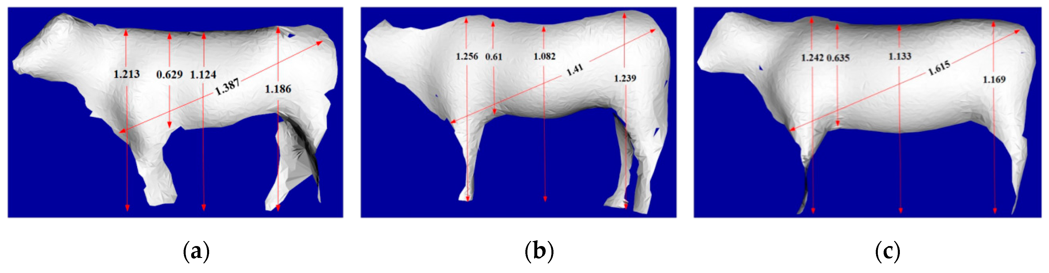
| Ear Tag of Cattle | Data Extraction Method and Error | Withers Height | Chest Depth | Back Height | Waist Height | Body Length |
|---|---|---|---|---|---|---|
| Q0392 | Automatic recognition | 1.213 | 0.629 | 1.124 | 1.186 | 1.387 |
| Human-machine interaction | 1.211 | 0.630 | 1.110 | 1.175 | 1.355 | |
| Error value | 0.17% | 0.16% | 1.26% | 0.94% | 2.36% | |
| Q0526 | Automatic recognition | 1.256 | 0.610 | 1.082 | 1.239 | 1.410 |
| Human-machine interaction | 1.255 | 0.619 | 1.095 | 1.237 | 1.414 | |
| Error value | 0.08% | 1.45% | 1.19% | 0.16% | 0.28% | |
| Q0456 | Automatic recognition | 1.242 | 0.635 | 1.133 | 1.169 | 1.615 |
| Human-machine interaction | 1.238 | 0.637 | 1.134 | 1.166 | 1.612 | |
| Error value | 0.32% | 0.31% | 0.09% | 0.26% | 0.19% |
© 2019 by the authors. Licensee MDPI, Basel, Switzerland. This article is an open access article distributed under the terms and conditions of the Creative Commons Attribution (CC BY) license (http://creativecommons.org/licenses/by/4.0/).
Share and Cite
Huang, L.; Guo, H.; Rao, Q.; Hou, Z.; Li, S.; Qiu, S.; Fan, X.; Wang, H. Body Dimension Measurements of Qinchuan Cattle with Transfer Learning from LiDAR Sensing. Sensors 2019, 19, 5046. https://doi.org/10.3390/s19225046
Huang L, Guo H, Rao Q, Hou Z, Li S, Qiu S, Fan X, Wang H. Body Dimension Measurements of Qinchuan Cattle with Transfer Learning from LiDAR Sensing. Sensors. 2019; 19(22):5046. https://doi.org/10.3390/s19225046
Chicago/Turabian StyleHuang, Lvwen, Han Guo, Qinqin Rao, Zixia Hou, Shuqin Li, Shicheng Qiu, Xinyun Fan, and Hongyan Wang. 2019. "Body Dimension Measurements of Qinchuan Cattle with Transfer Learning from LiDAR Sensing" Sensors 19, no. 22: 5046. https://doi.org/10.3390/s19225046