Multifunctional Medical Recovery and Monitoring System for the Human Lower Limbs


Abstract
:1. Introduction
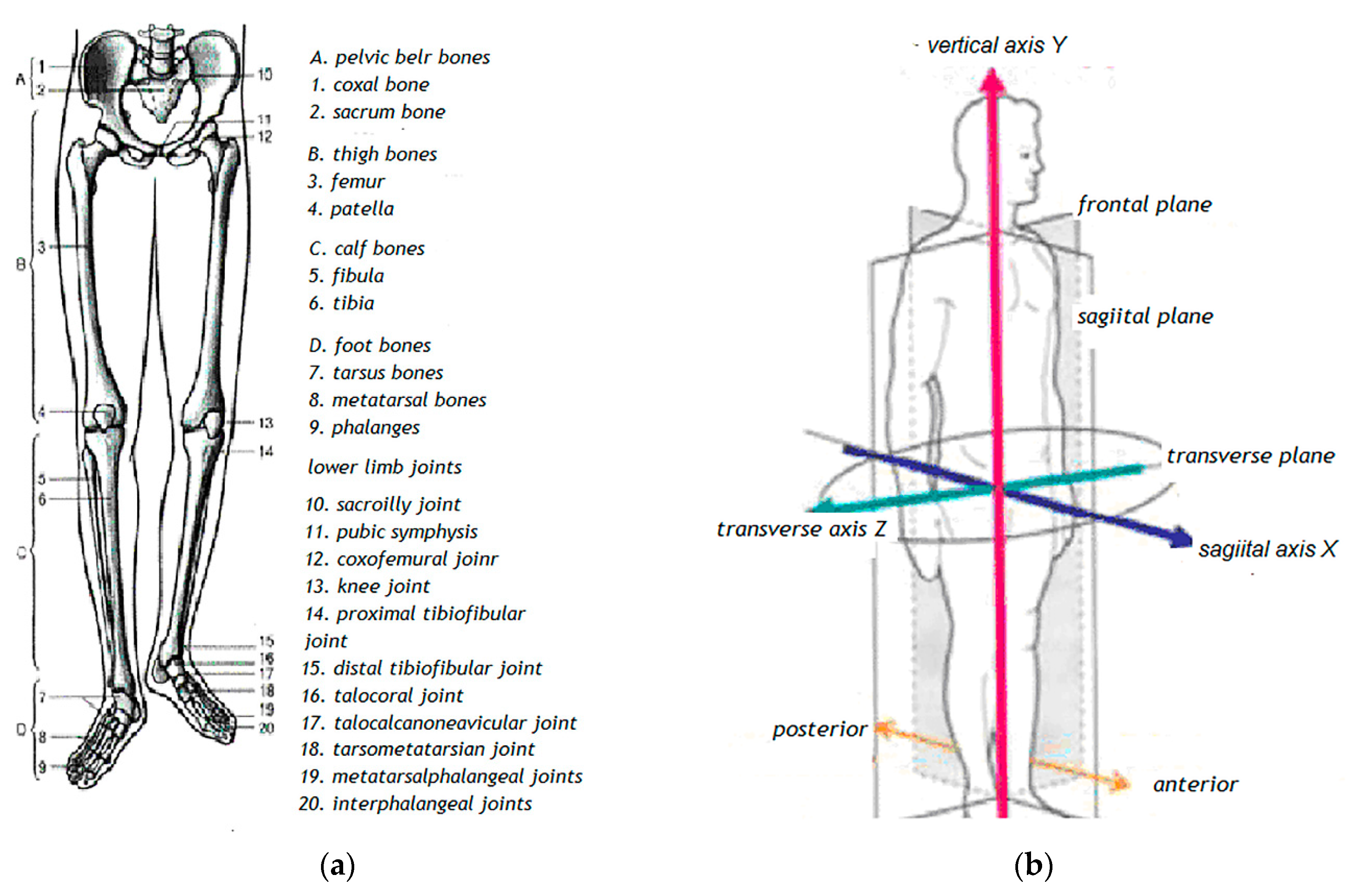
2. The Structural Model of the Human Lower Limb
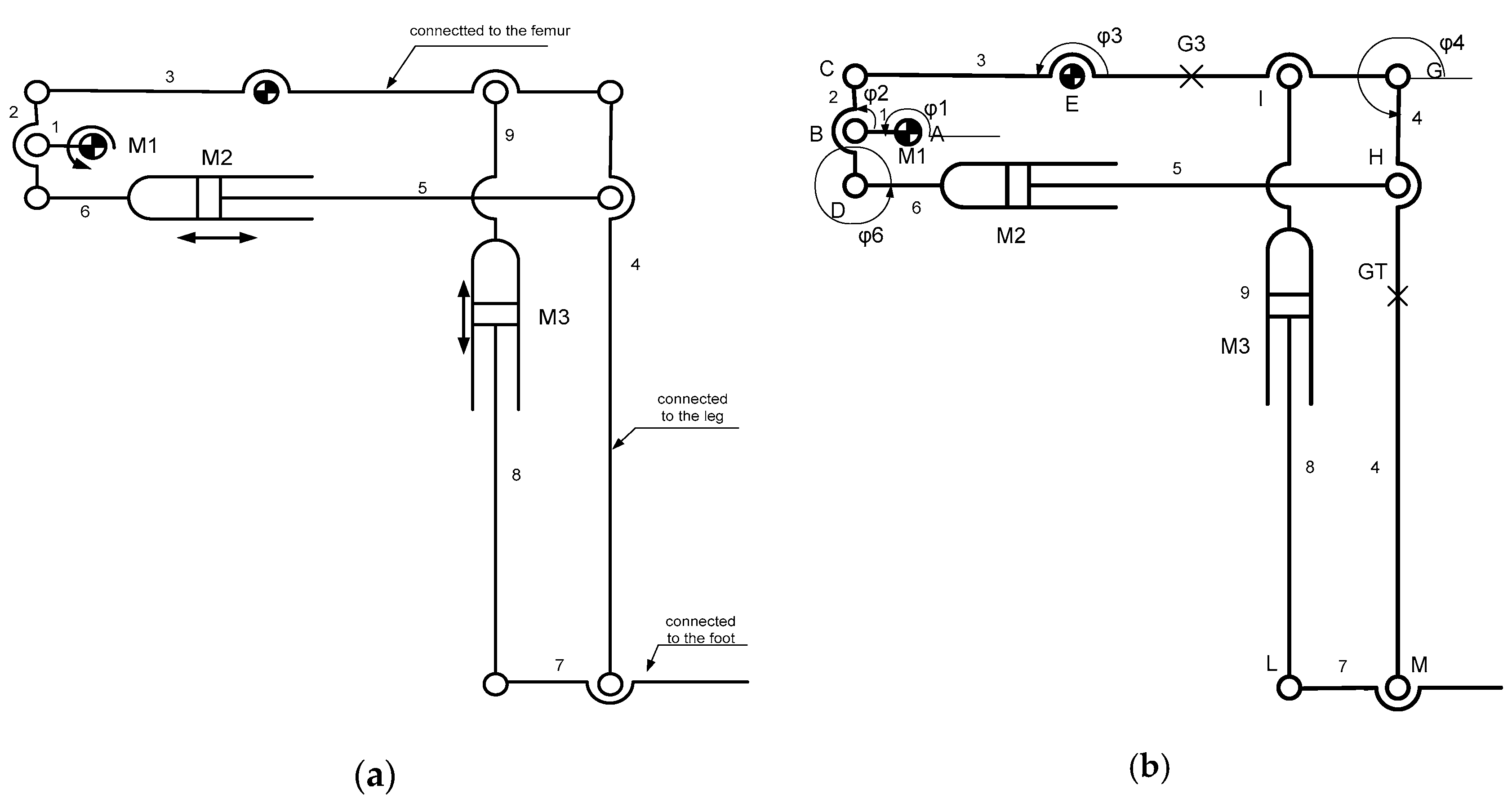
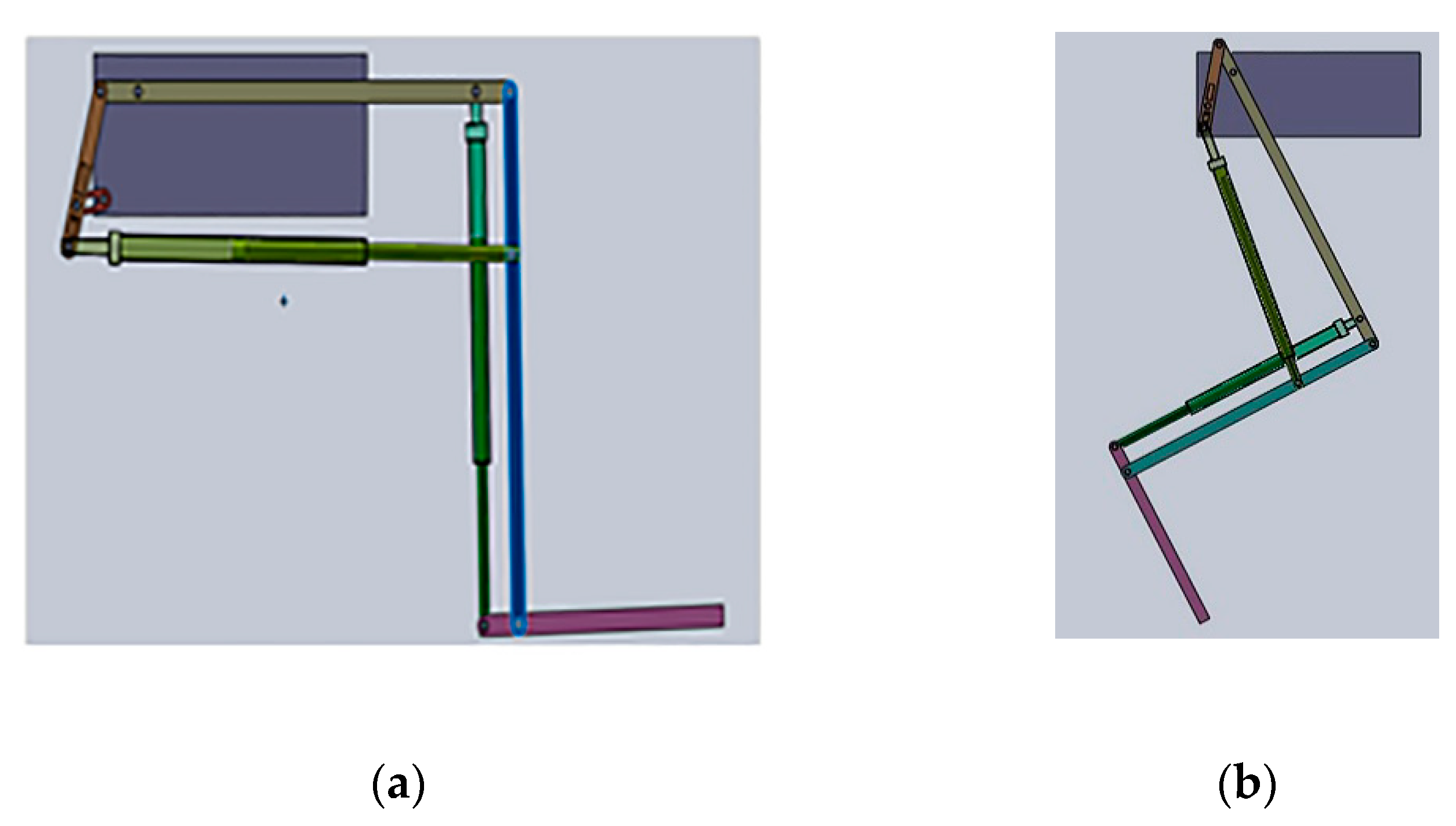
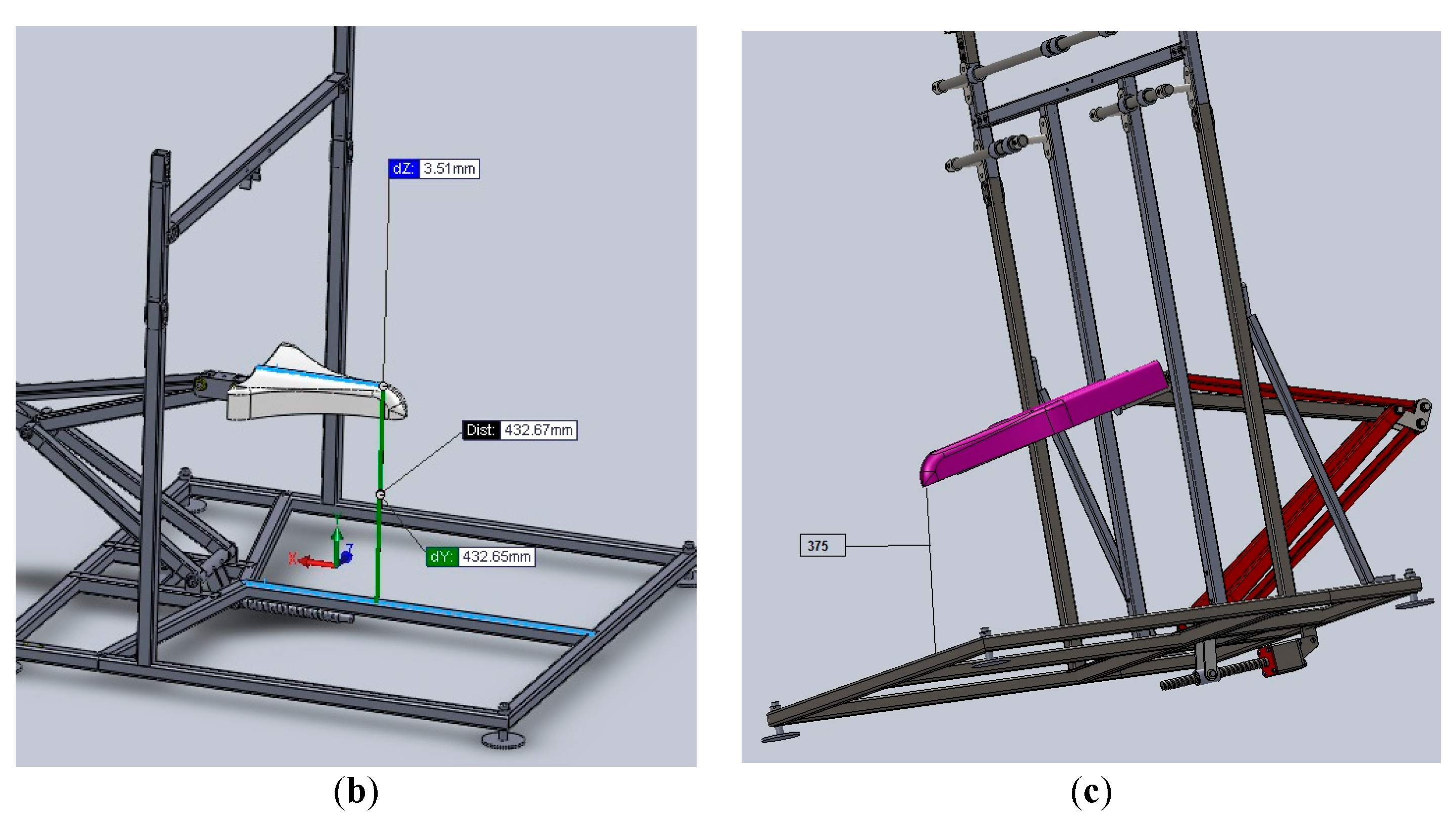
- It is necessary to use all active pairs to exclusively exercise the coxofemural joint. M1 ensures the motion of the femur relative to the trunk, when M2 and M3 maintain the relative fixed position of the leg and foot. The connection presented in Figure 3b is available and can be applied to estimate the characteristics of all active pairs.
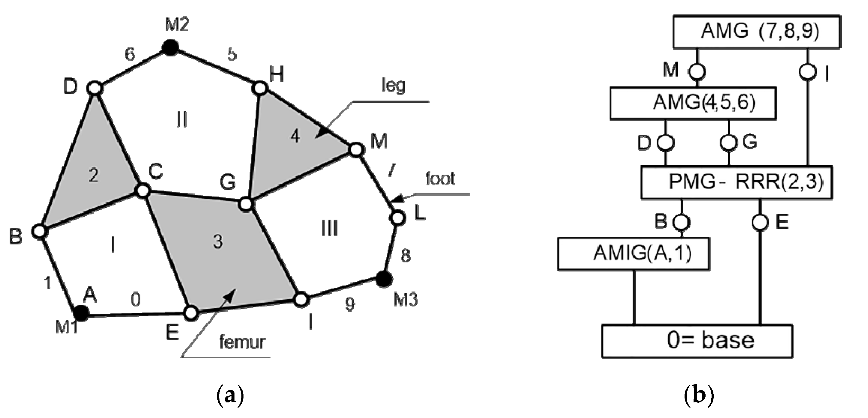
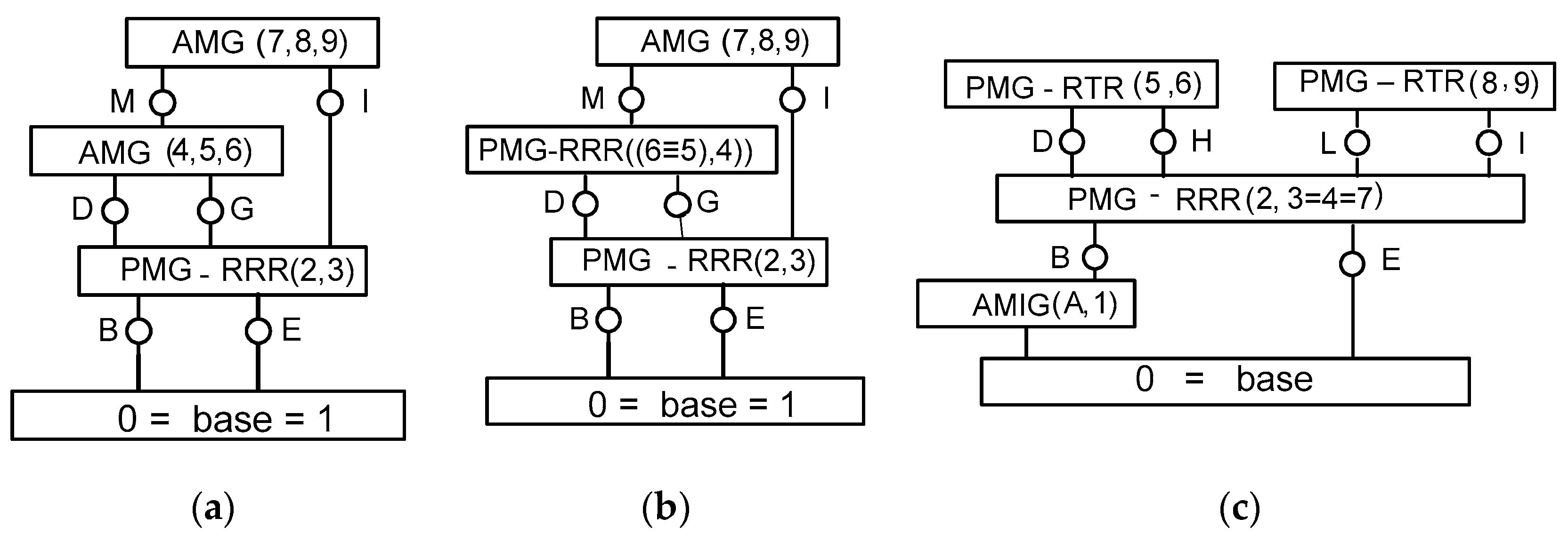
- In order to exclusively move the knee joint, M1 is blocked in the desired position. At the same time, M3 ensures the position of the foot relative to the leg. M2 determines the motion of the knee. The modular configuration is given in Figure 4a. In its construction, it has a single modular passive group (Table 1) denoted by RRR (2, 3) and two active ones (Table 2) given by AMG–RTRR (4, 5, 6) and AMG–RTRR (7, 8, 9).
- To act only the talocrural joint according to the medical parameters maintaining in the convenient fixed position the leg and the foot, the active pairs M1 and M2 are used to place the human member segments in the desired positions and M3 to determine the movement of the foot. The modular configuration for this section is shown in Figure 4b. Two modular passive groups given by PMG–RRR (2, 3) and PMG–RRR ((6 ≡ 5), 4) and a single mono-mobile one marked AMG–RTRR (7, 8, 9) are relevant for the proposed purpose. In the following, there are various cases of using the mechanism for functional recovery of the lower human joints.
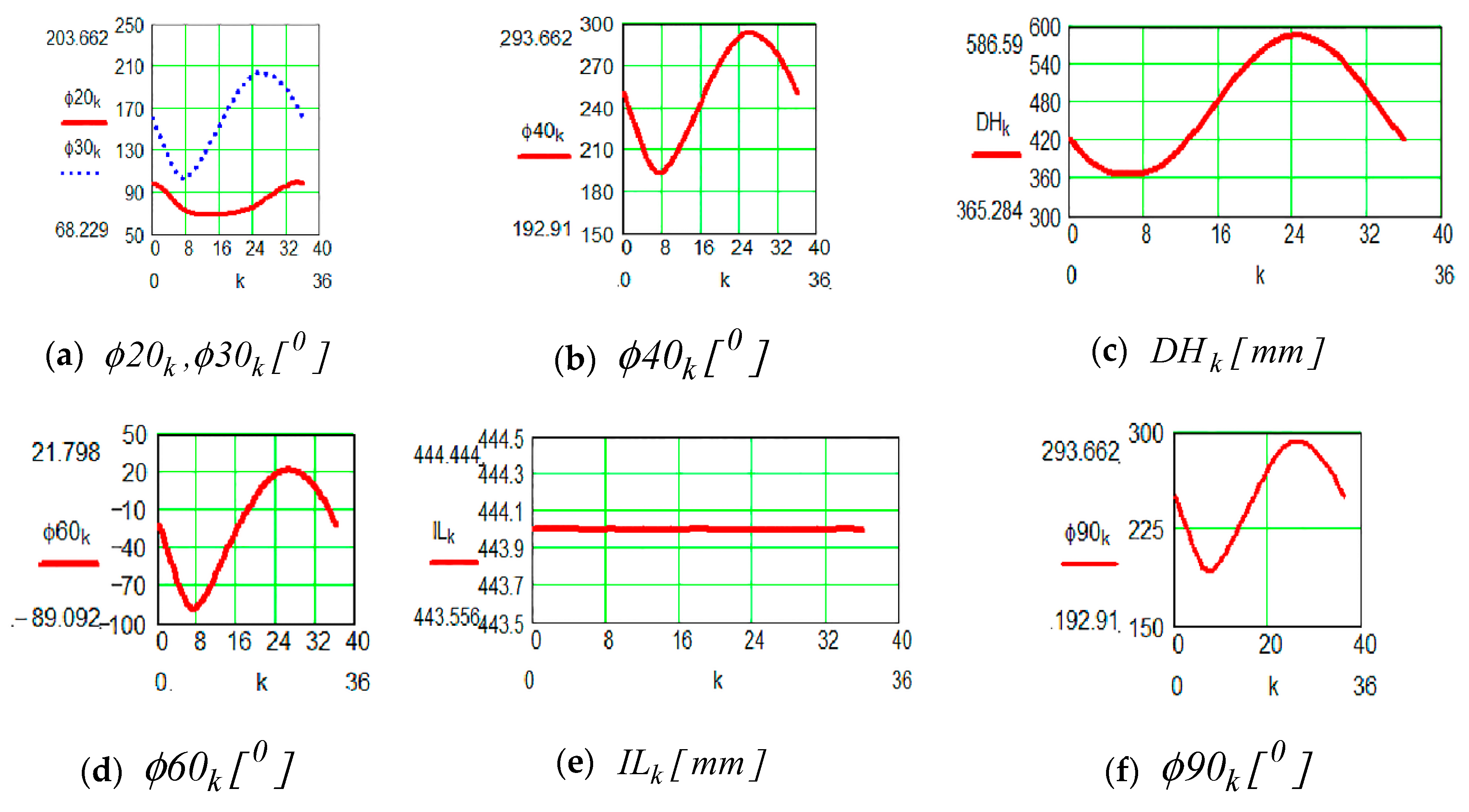
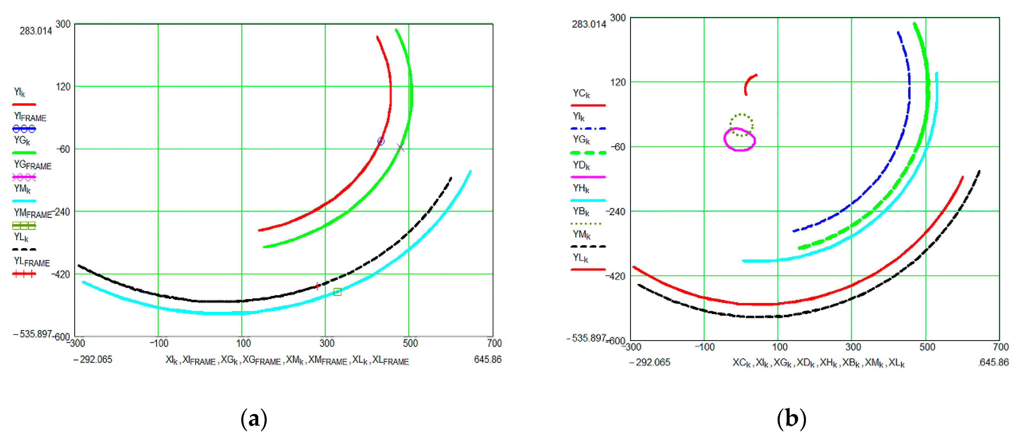
3. Mechanism Kinematic Characteristics for the Exclusive Recovery of the Coxofemural Joint Function
4. Mechanism Dynamic Characteristics for the Coxofemoral Joint Function Recovery
5. Mechanism Characteristics for the Knee Joint Function Exclusive Recovery
6. Mechanism Characteristics for the Talocrural Joint Exclusive Recovery
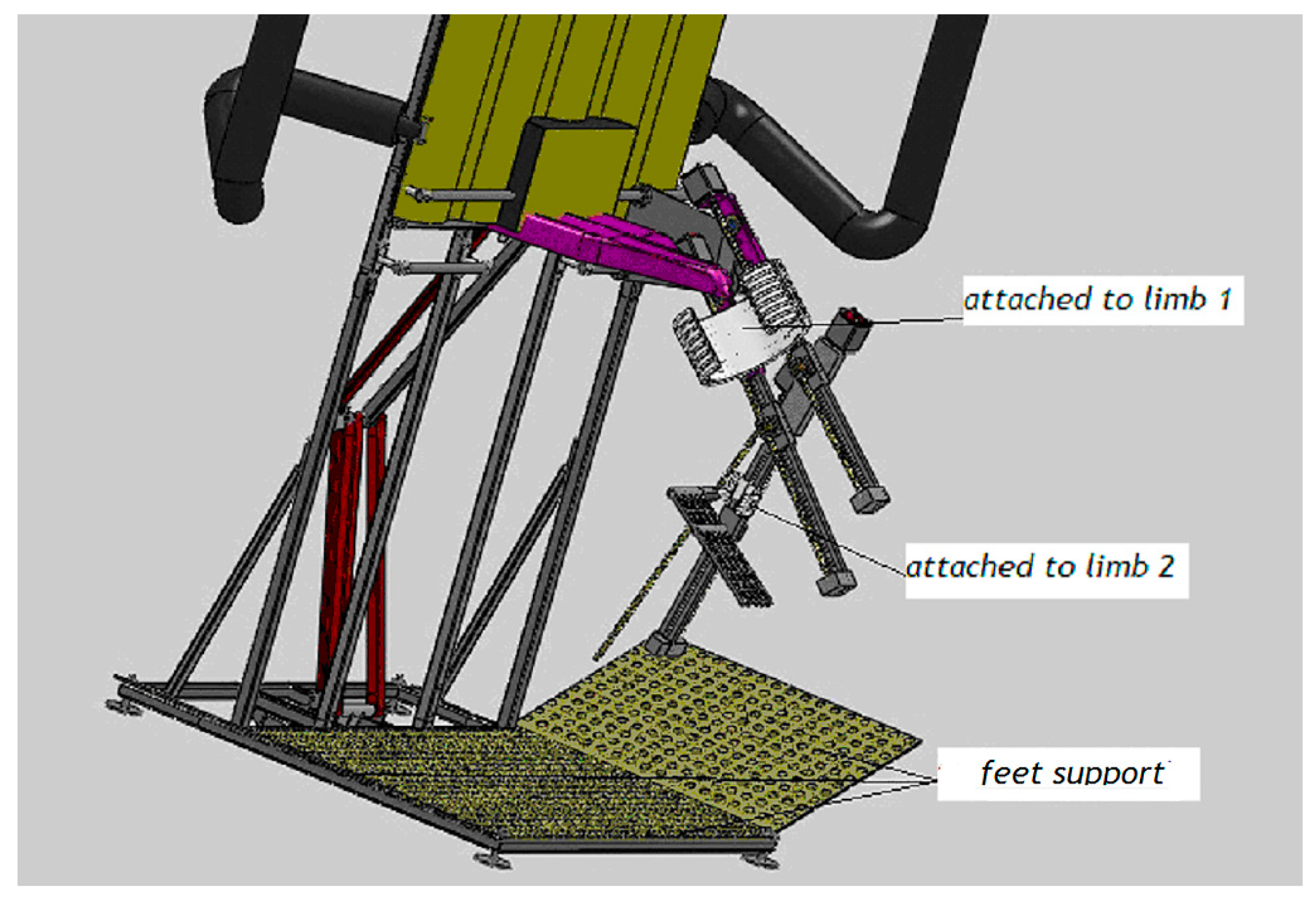
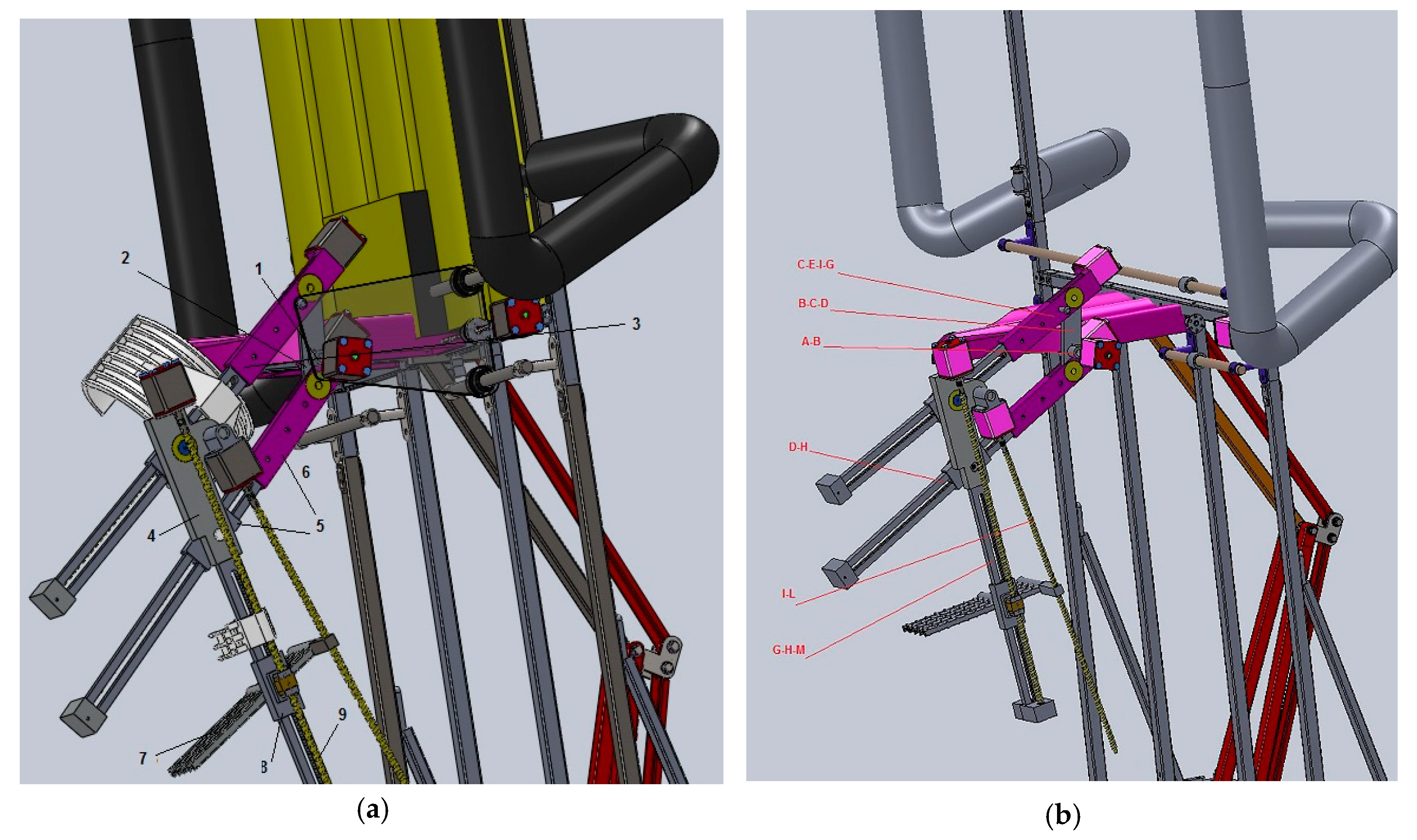
7. Multifunctional Medical System for Recovery and Monitoring of the Lower Limb
8. Discussion
9. Conclusions
Author Contributions
Funding
Conflicts of Interest
References
- Comanescu, A.; Banica, E.; Comanescu, D. Human Inferior Member Model for a Medical Functional System. In Proceedings of the 8th World Congress of Biomechanics, Dublin, Ireland, 8–12 July 2018. [Google Scholar]
- Comanescu, A.; Comanescu, D.; Dugaesescu, I.; Ungureanu, L.; Alionte, C. Mechanisms and Bio-Morph System Modeling and Simulation (Modelarea şi Simularea Mecanismelor şi Sistemelor Biomorfe); POLITEHNICA Press, POLITEHNICA University of Bucharest: Bucharest, Romania, 2019; Chapter 2,3,12; ISBN 978-606-515-857-3. [Google Scholar]
- Aparat pentru recuperare glezna. Available online: https://www.help-devices.ro/Aparat-pentru-recuperare-glezna-68.html (accessed on 10 January 2018).
- Dispozitiv reeducare flexie, extensie, pronatie, supinatie picior in paralizii de sciatic popliteu extern si intern cod 07755. Available online: https://www.help-devices.ro/Dispozitiv-reeducare-flexie-extensie-pronatie-supinatie-picior-in-paralizii-de-sciatic-popliteu-extern-si-intern-cod-07755-69.html (accessed on 10 January 2018).
- Available online: https://www.help-devices.ro/mini-stepper-66.html (accessed on 10 March 2018).
- Minitalus. Available online: https://www.help-devices.ro/Minitalus-224.html (accessed on 10 January 2018).
- CPM machine/knee CPM. Available online: https://www.alibaba.com/product-detail/CPM-machine-knee-CPM_60477429672.html (accessed on 10 January 2018).
- 4621006502 KINETEC BREVA ANKLE CPM. Available online: https://neotech.ro/4621006502-kinetec-breva-ankle-cpm/208.htm (accessed on 10 March 2018).
- Dragne, V. Recovering and Monitoring System for the Lower Human Member. Master’s Thesis, POLITEHNICA University of Bucharest, Bucharest, Romania, 2017. [Google Scholar]
- Cioaga, P.B. Command System Characteristics of a Multifunctional Recovering Apparatus for the Lower Human Member. Master’s Thesis, Politehnica University of Bucharest, Bucharest, Romania, 2017. [Google Scholar]
- Bataller, J.A.; Cabrera, M.; Clavijo, M.; Castillo, J.J. Evolutionary Synthesis of Mechanisms Applied to the Design of an Exoskeleton for Finger Rehabilitation. Mech. Mach. Theory 2016, 105, 31–43. [Google Scholar] [CrossRef]
- Yang, W.; Ding, H.; Kecskeméthy, A. Automatic Synthesis of Plane Kinematic Chains with Prismatic Pairs and up to 14 Links. Mech. Mach. Theory 2019, 132, 236–247. [Google Scholar] [CrossRef]
- Castro, M.N.; Rasmussen, J.; Andersen, M.S.; Bai, S. A Compact 3-DOF Shoulder Mechanism Constructed with Scissors linkages. Mech. Mach. Theory 2019, 132, 264–278. [Google Scholar] [CrossRef]
- Peña-Pitarch, E.; Falguera, N.T.; Martinez, J.A.L.; Al Omar, A.; Larrión, I.A. Driving Devices for a Hand Movement without External Force. Mech. Mach. Theory 2016, 105, 388–396. [Google Scholar] [CrossRef]
- Angeles, J. Fundamentals of Robotic Mechanical Systems: Theory, Methods and Algorithms; Springer: New York, NY, USA, 2003. [Google Scholar]
- Bishop, R.H. The Mechatronics Handbook; CRC Press: Boca Raton, FL, USA, 2002. [Google Scholar]
- Rojas, N.; Thomas, F. On closed-form solutions to the position analysis of Baranov trusses. Mech. Mach. Theory 2012, 50, 179–196. [Google Scholar] [CrossRef]
- Ramakrishna, K.; Sen, D. Form-closure of Planar Mechanisms. Synthesis of Number, Configuration and Geometry of Point Contacts. Mech. Mach. Theory 2018, 130, 220–243. [Google Scholar]
- Rai, R.K.; Punjabi, S. A New Algorithm of Links Labelling for the Isomorphism Detection of Various Kinematic Chains Using Binary Code. Mech. Mach. Theory 2019, 131, 1–32. [Google Scholar] [CrossRef]
- Glowinski, S.; Krzyzynski, T. An inverse kinematic algorithm for the human leg. J. Theor. Appl. Mech. 2016, 54, 53–61. [Google Scholar] [CrossRef]


| Baranov Truss (BT) System with Three Degree of Freedom and Zero Degree of Mobility | Passive Modular Group (PMG) System with Zero Degree of Mobility | |
|---|---|---|
 BT 1 |  | PMG 1 |
 BT 2 |  | PMG 2 |
 | PMG 3 | |
 BT 3 |  | PMG 5 |
 | PMG 9 | |
 | PMG 11 | |
 BT 4 |  | PMG 6 |
 | PMG 8 | |
 | PMG 10 | |
 | PMG 12 | |
 BT 5 |  | PMG 4 |
 | PMG 7 | |
 | PMG 13 | |
 |  |  |  |
 |  |  |  |
| Coordinates of the A and E Pairs Relative to the Fixed Reference System | |
|---|---|
| AB | 30 |
| BC | 115 |
| BD | 42.39 |
| CE | 40 |
| EG | 456 |
| EI | 456–50 |
| EG3 G3—mass center of the 3 link—femur | 152 |
| MG | 444 |
| GGT GT—mass center of the 4 link—leg | 444–296 |
| GH | 151 |
| LM | 50 |
| MGL GL—mass center of the 7 link—foot | 150 |
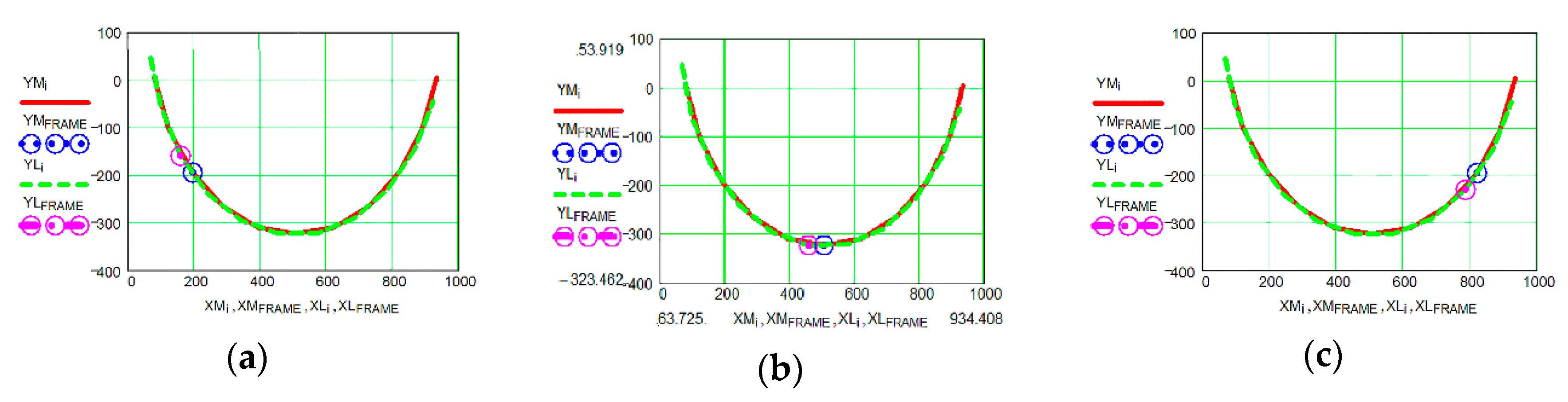
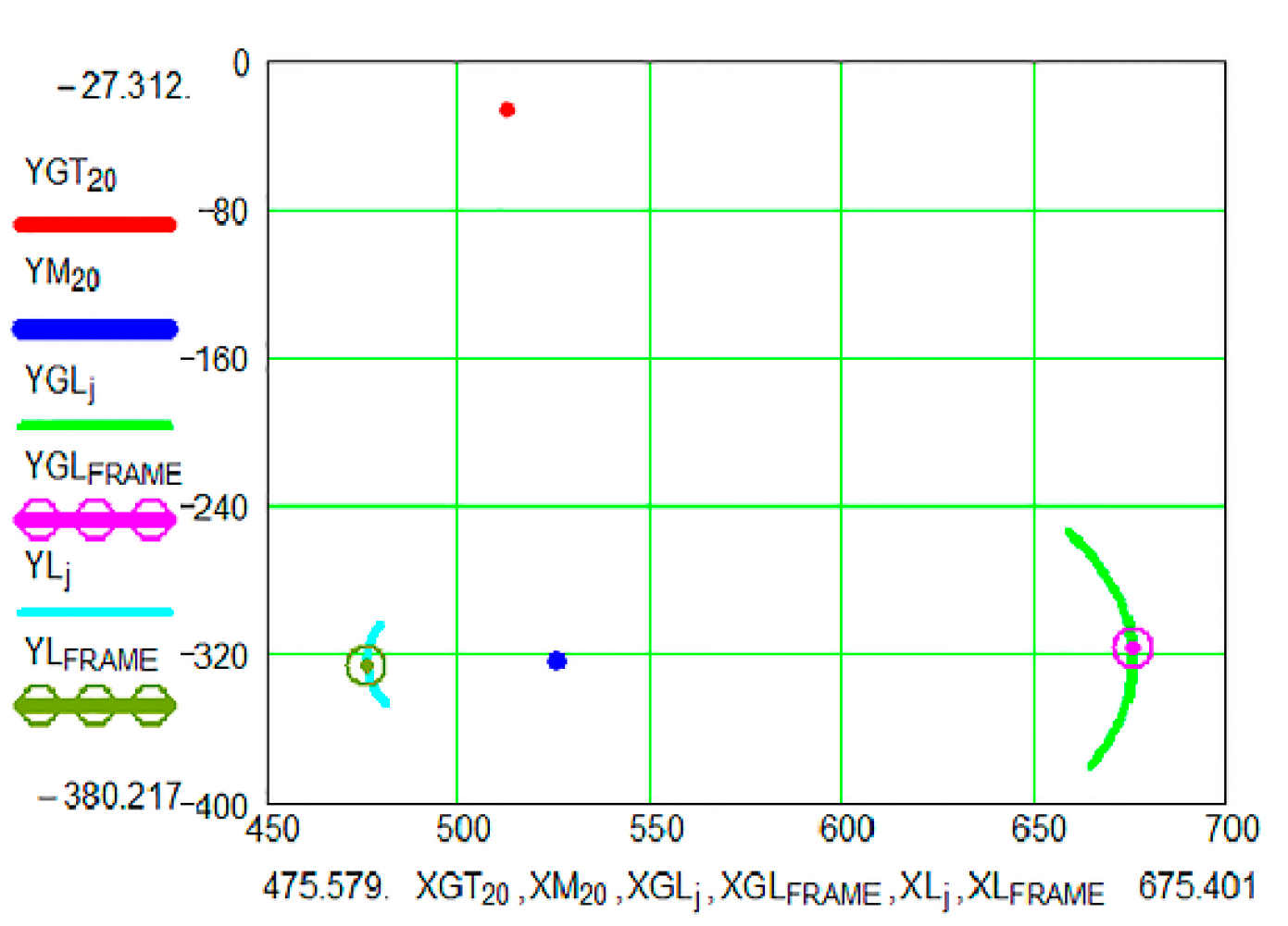
| Dependent Parameters (Figure 2) | Positional Dependent Parameters Determination Algorithm |
|---|---|
| B (XB, YB) kinematic pair B coordinates | |
| angular parameters for PMG (2,3)–RRR (2,3) | -values in rad., -values in 0. |
| C (XC, YC) kinematic pair C coordinates | |
| D (XD, YD) kinematic pair D coordinates | |
| I (XI, YI) kinematic pair I coordinates | |
| G (XG, YG) kinematic pair G coordinates | |
| M (XM, YM) kinematic pair M coordinates | |
| H (XH, YH) kinematic pair H coordinates | |
| L (XL, YL) kinematic pair L coordinates | |
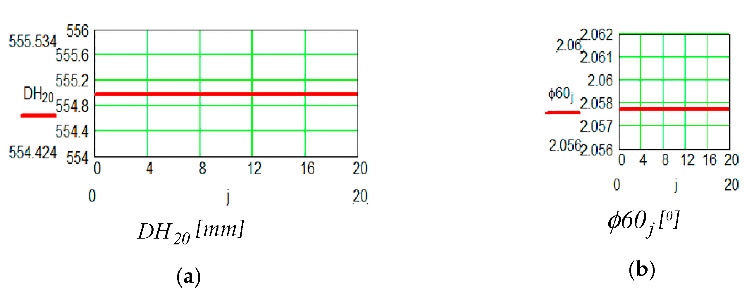
| parameters for PMG (6, 5) = RTR (6, 5) DH–linear parameter, -angular parameter | |
| ϕ6k = τk, ϕ60k- values in 0 of the ϕ6k in rad. | |
parameters for PMG (9, 8) = RTR (9, 8) IL–linear parameter, -angular parameter | |
| -values in 0 of the in rad. | |
| G3 (XG3, YG3) coordinates of the 3 link-femur center of mass G3 | |
| G3–the 3 link–femur centre of mass. | |
| GT (XGT, YGT) coordinates of the 4 link-leg center of mass GT | |
| GT–the 4 link–leg centre of mass. | |
| GL (XGL, YGL) coordinates of the 7 link-foot center of mass GL | |
| GL–the 7 link–foot centre of mass. | |
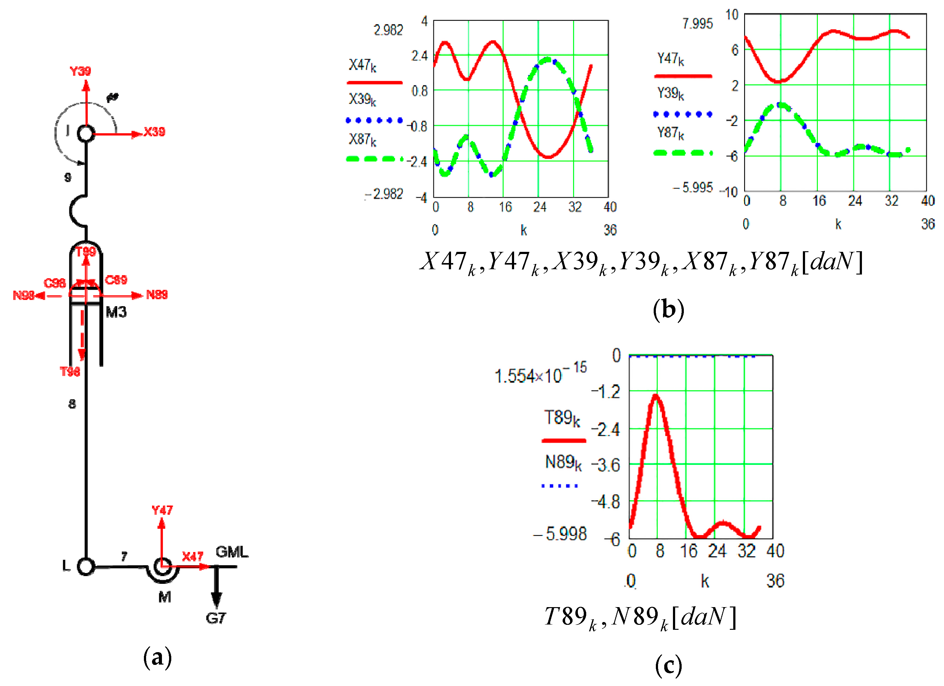
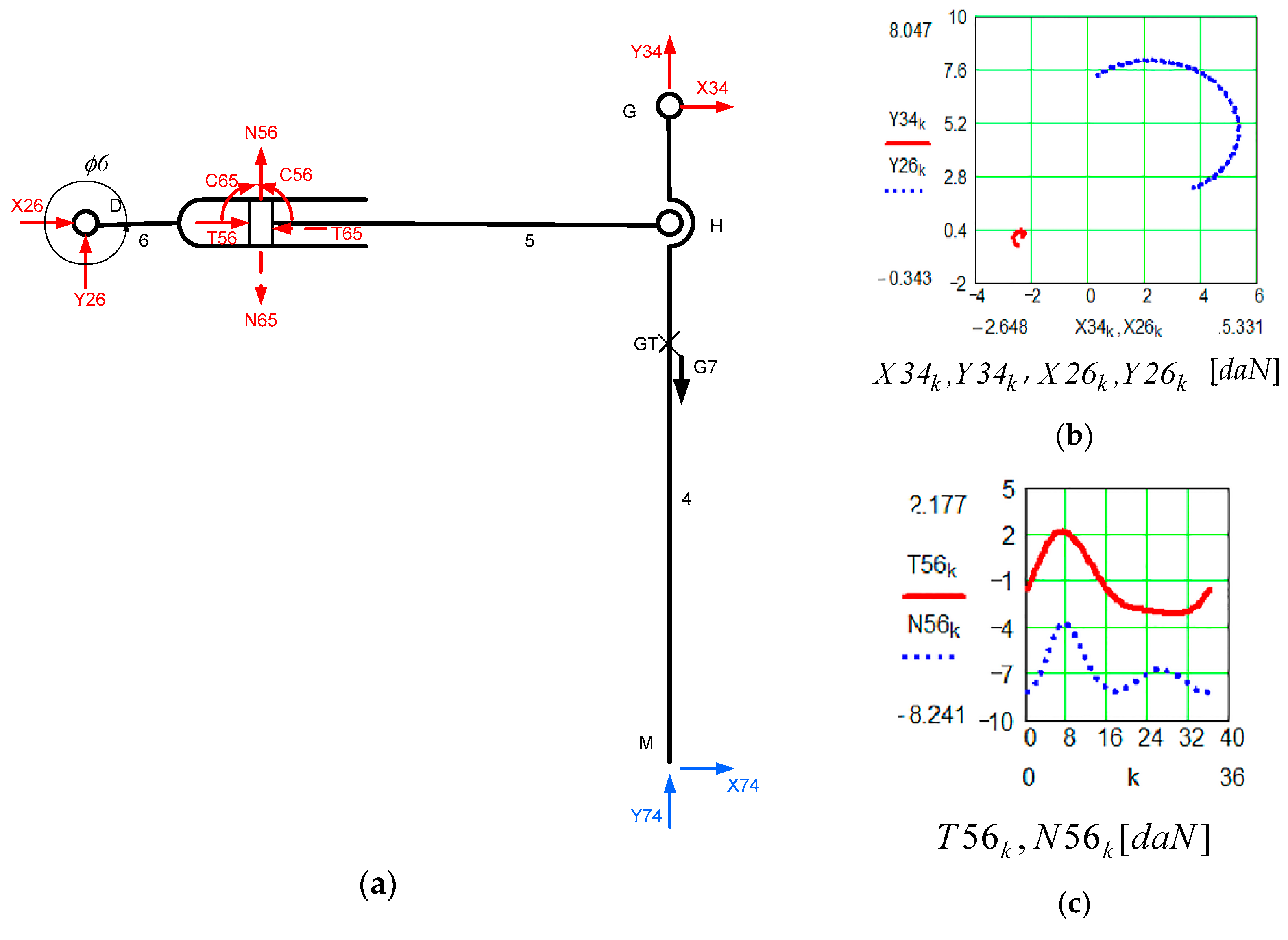
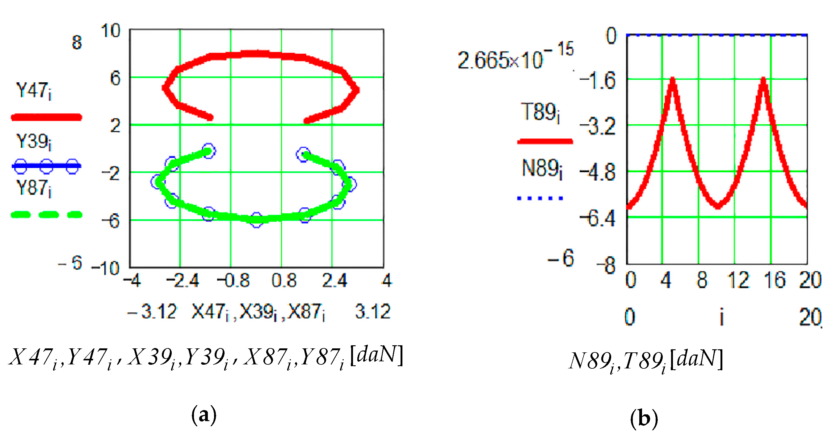
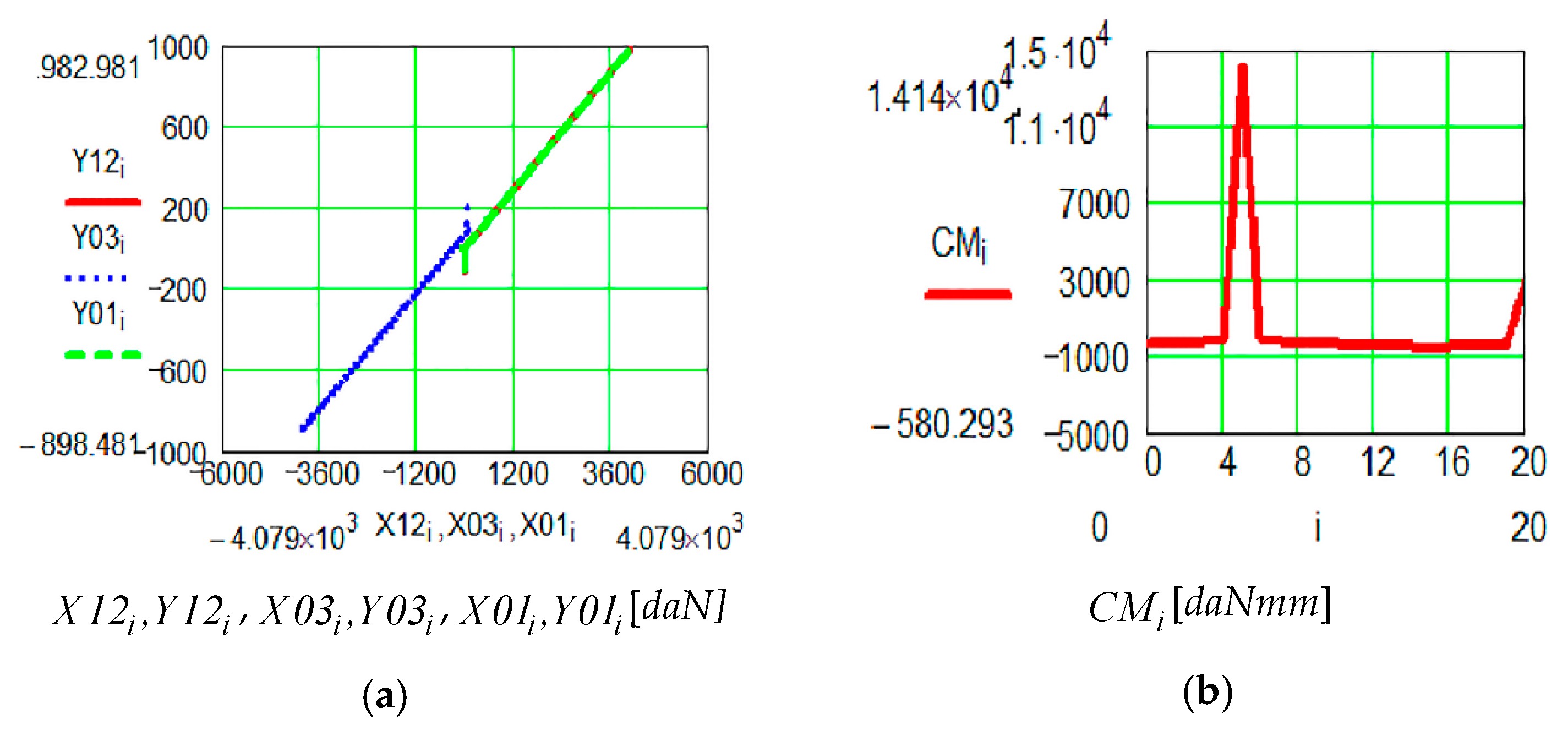
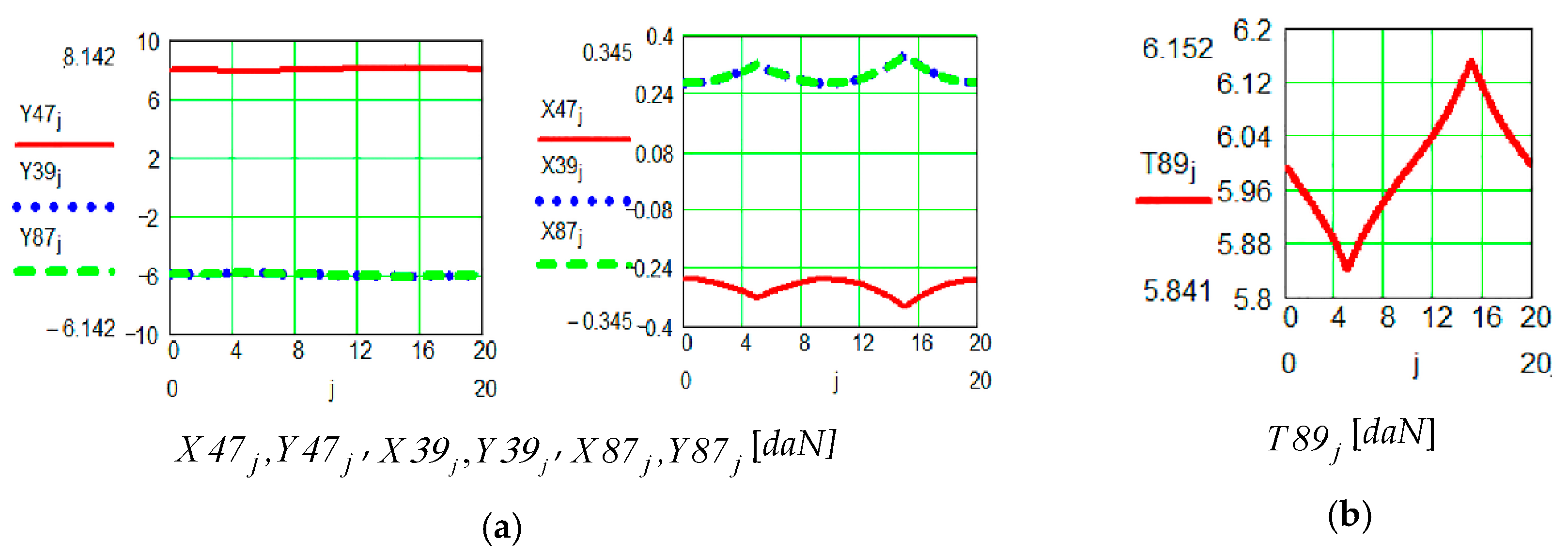
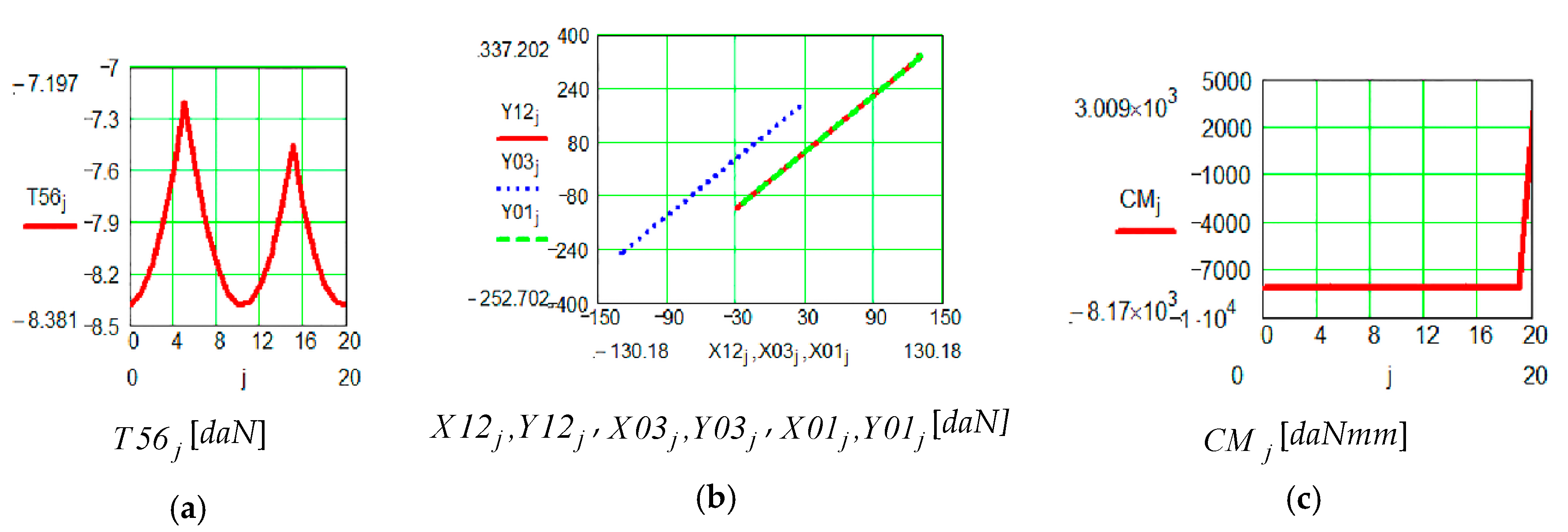
| RTRR (9, 8, 7) | The equivalent torque of the external and inertial forces for link 7 vidi Figure 8 | X7 = 0 Y7 = −G7 CM7 = 0 | |
| G7-link 7 weight-Mass and moment of inertia for links 9 and 8 are neglected | |||
| The reaction torque in pair M vidi Figure 8 ; ; | |||
| The reaction torque in pair I vidi Figure 8 ; ; | |||
| The reaction torque in pair L vidi Figure 8 | |||
| The reaction torque in active pair M3 vidi Figure 8 | |||
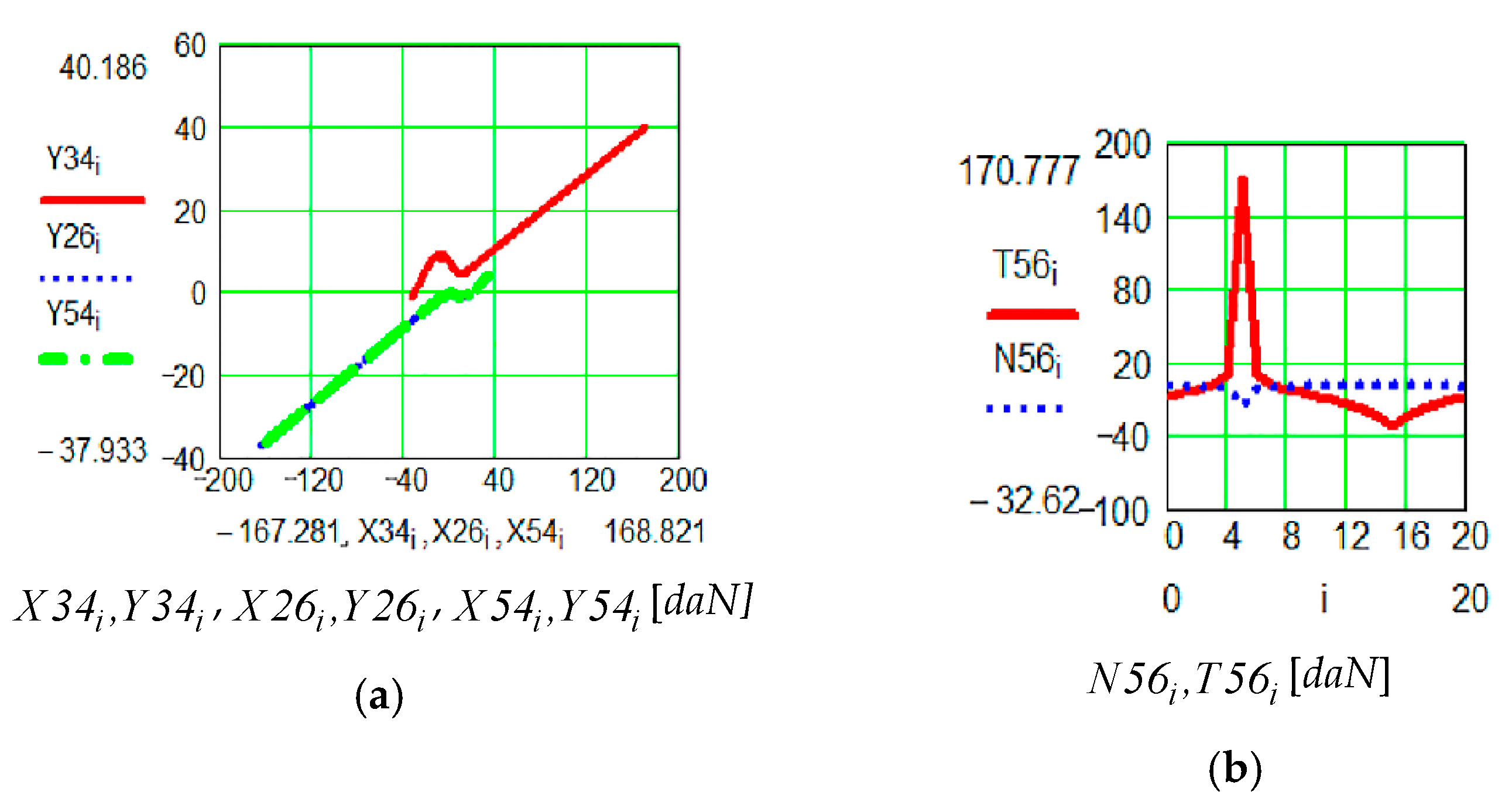
| RTRR (6, 5, 4) | The equivalent torque of the external and inertial forces for link 4 | ||
| The reaction torque in pair G vidi Figure 9 | |||
| The reaction torque in pair D vidi Figure 9 | |||
| The reaction torque in pair H vidi Figure 9 | |||
| The reaction torque in active pair M2 vidi Figure 9 | |||
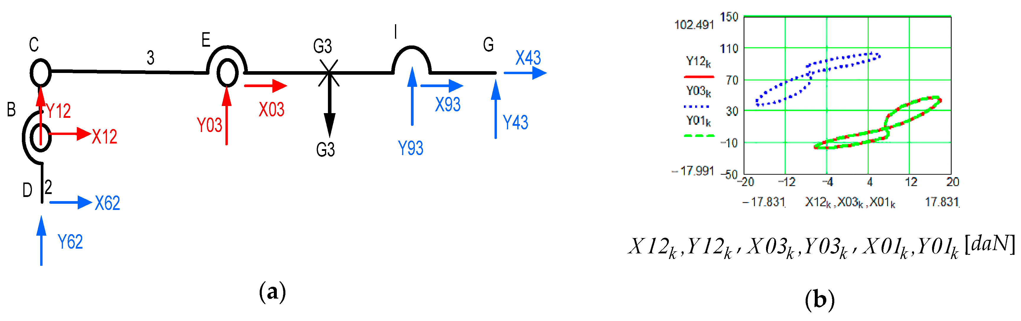
| RRR (2, 3) | G2 center of mass coordinates vidi Figure 10 | ||
| The equivalent torque of the external and inertial forces for link 2 vidi Figure 10 | |||
| The equivalent torque of the external and inertial forces for link 3 vidi Figure 10 | |||
| -link 3 weight | |||
| The reaction torque in pair B vidi Figure 10 | |||
| The reaction torque in pair E vidi Figure 10 | |||
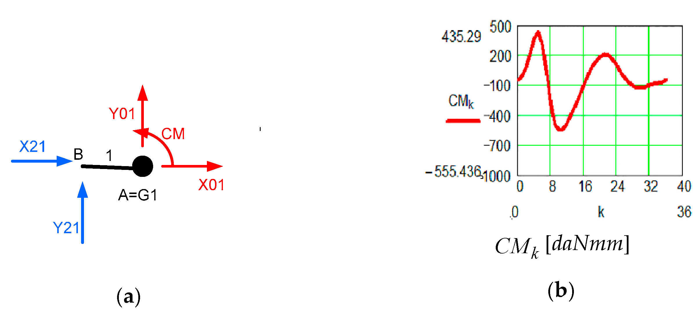
| AMIG (A, 1) | The reaction torque in active pair A vidi Figure 11 | ,
, |
| M1 Active Pair | ||
 |  | |
| Positional characteristic [0] | Dynamic characteristic [daNmm] | |
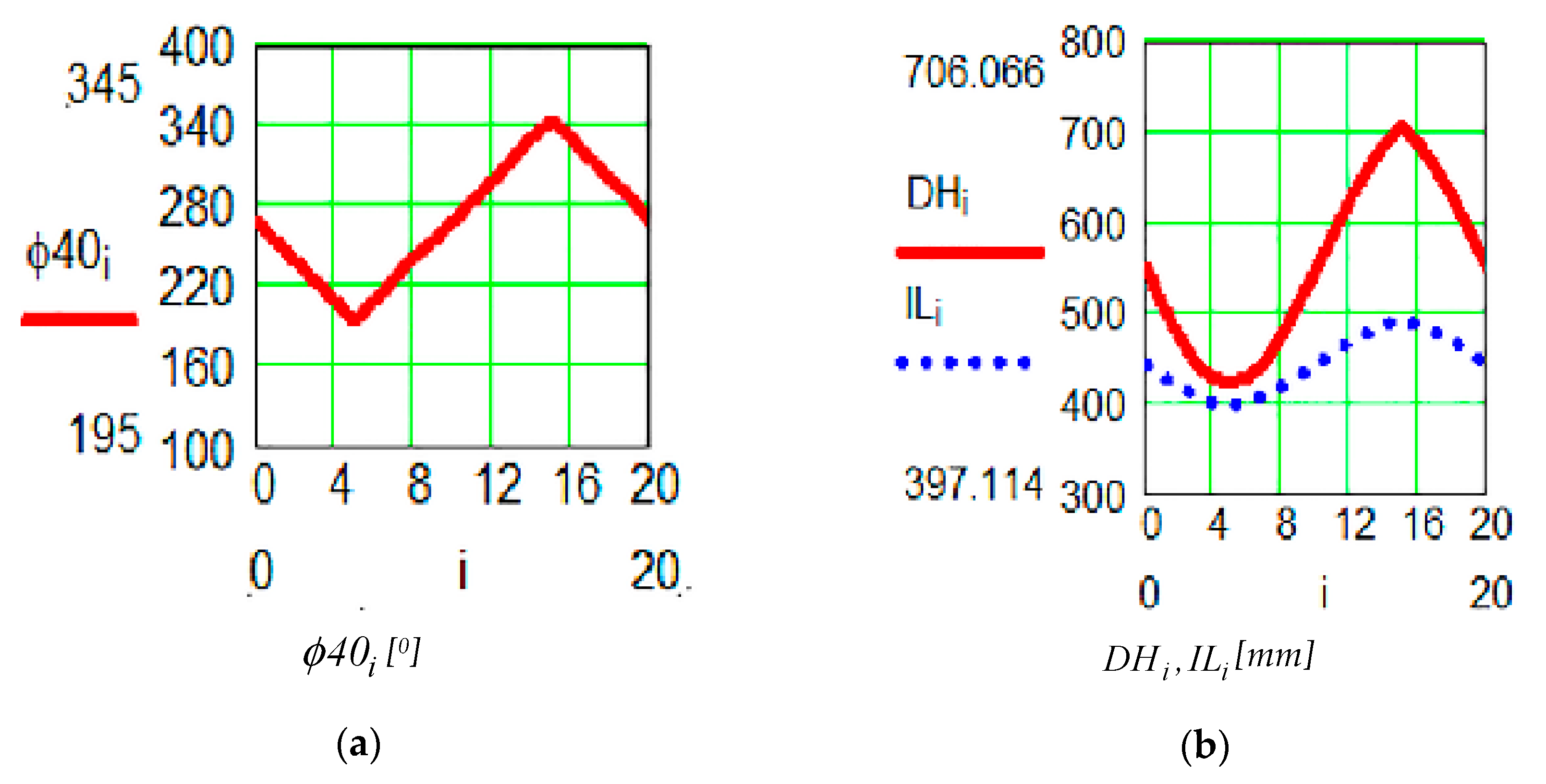
| M2 Active Pair | ||
‘  |  | |
| Positional characteristic [mm] | Dynamic characteristic [daN] | |
| M3 Active Pair | ||
 |  | |
| Positional characteristic [mm] | Dynamic characteristic [daN] | |
| M1 Active Pair | ||
 |  | |
| Positional characteristic [0] | Dynamic characteristic [daNmm] | |
| M2 Active Pair | ||
 |  | |
| Positional characteristic [mm] | Dynamic characteristic [daN] | |
| M3 Active Pair | ||
 |  | |
| Positional characteristic [mm] | Dynamic characteristic [daN] | |
| M1 Active Pair | ||
 |  | |
| Positional characteristic [0] | Dynamic characteristic | |
| M2 Active Pair | ||
 |  | |
| Positional characteristic | Dynamic characteristic | |
| M3 Active Pair | ||
 |  | |
| Positional characteristic | Dynamic characteristic | |
© 2019 by the authors. Licensee MDPI, Basel, Switzerland. This article is an open access article distributed under the terms and conditions of the Creative Commons Attribution (CC BY) license (http://creativecommons.org/licenses/by/4.0/).
Share and Cite
Comanescu, A.; Dugaesescu, I.; Boblea, D.; Ungureanu, L. Multifunctional Medical Recovery and Monitoring System for the Human Lower Limbs. Sensors 2019, 19, 5042. https://doi.org/10.3390/s19225042
Comanescu A, Dugaesescu I, Boblea D, Ungureanu L. Multifunctional Medical Recovery and Monitoring System for the Human Lower Limbs. Sensors. 2019; 19(22):5042. https://doi.org/10.3390/s19225042
Chicago/Turabian StyleComanescu, Adriana, Ileana Dugaesescu, Doru Boblea, and Liviu Ungureanu. 2019. "Multifunctional Medical Recovery and Monitoring System for the Human Lower Limbs" Sensors 19, no. 22: 5042. https://doi.org/10.3390/s19225042