Data Mining and Statistical Approaches in Debris-Flow Susceptibility Modelling Using Airborne LiDAR Data

Abstract

Cameron Highland is a popular tourist hub in the mountainous area of Peninsular Malaysia. Most communities in this area suffer frequent incidence of debris flow, especially during monsoon seasons. Despite the loss of lives and properties recorded annually from debris flow, most studies in the region concentrate on landslides and flood susceptibilities. In this study, debris-flow susceptibility prediction was carried out using two data mining techniques; Multivariate Adaptive Regression Splines (MARS) and Support Vector Regression (SVR) models. The existing inventory of debris-flow events (640 points) were selected for training 70% (448) and validation 30% (192). Twelve conditioning factors namely; elevation, plan-curvature, slope angle, total curvature, slope aspect, Stream Transport Index (STI), profile curvature, roughness index, Stream Catchment Area (SCA), Stream Power Index (SPI), Topographic Wetness Index (TWI) and Topographic Position Index (TPI) were selected from Light Detection and Ranging (LiDAR)-derived Digital Elevation Model (DEM) data. Multi-collinearity was checked using Information Factor, Cramer’s V, and Gini Index to identify the relative importance of conditioning factors. The susceptibility models were produced and categorized into five classes; not-susceptible, low, moderate, high and very-high classes. Models performances were evaluated using success and prediction rates where the area under the curve (AUC) showed a higher performance of MARS (93% and 83%) over SVR (76% and 72%). The result of this study will be important in contingency hazards and risks management plans to reduce the loss of lives and properties in the area.

1. Introduction

Rapid population growth and its increasing concentration in urban areas have worsened the severity and impact of gravity-induced disasters across the globe, particularly in the mountainous environment. Debris flow is a natural hazard that occurs in a valley or on a mountain slope destroying everything it passes through. Debris flows occur when poorly sorted sediment, agitated and saturated with water, surge down-slopes due to the gravitational force, deposit on mountain bottom to form fans [1,2]. Iverson [3] defined debris flows as “turbulent flowing mixtures of sediment and liquid in nearly equal proportions”. Depending on the types of material involved, debris flows are variously known as mud spates, mudslides, mudflows, debris torrents, debris slides, debris floods, lahar and hyper-concentrated flows [2]. The ratios of solid and liquid constituents present in the mechanics of earth movements differentiate debris-flow events from other related phenomena. Accordingly, based on solid-liquid ratio contents one can easily categorize the type of events. In view of these, if solid sediment controls the liquid content, the constituent formed is avalanche; whereas if liquid forces control the solid content that results in floods, on the other hand, when an equal concert of liquid and solid presents it is formed as debris flows [3]. This forms a discern transition between avalanches and floods, based on their geological type and mechanical conduct characteristic [2]. In view of this, both solid and liquid (fluid) forces extremely influence the motion of debris flow, which could be responsible for its uniquely destructive power. Debris flow can be mobilized by either old or new landslides in the upper slopes that transport a mixture of equal quantity of grains (sediments) and fluid in high density verged downslope to a valley deposition zone, where the effects are usually felt on human economic development and social safety. Consequently, resulted in the loss of life and property. The event usually triggered by a number of factors such as heavy precipitation, lahar, earthquake, landslide and other anthropogenic activities [4,5,6,7,8,9,10]. Noteworthy, the prominent factors trigger debris-flow events in Malaysia is torrential rainfall that transforms landslides to a ribbon of surge liquid and solid sediments forming the debris flows [11]. Flows at high velocity along hill slopes and valleys exposing the regions to great risk of debris flow which results in a huge number of casualties and property damage along its path [8,12,13]; as the region suffers a frequent revisit period. A study by Berti et al. [14] estimated the reoccurrence periods for moderate debris flows to be a single occurrence in every two to three years interlude.

The hydrological factor of debris flow initiation (shallow slope failure, advancing erosion, activated by runoff), normally determines the action of runoff to precipitation of the unstable slope [15]. This event could be triggered by an influx of rapid concentration of fluid in the pebbly sinks that lack flora and soil; excessive overflow seepage rapidly transported at the sink channel where transient outlets incised into scree-covered slopes. Hence debris-flow events can be originated on such waterways at any sufficient runoff to activate free seepage solid grains of the channel bed [15,16]. So also, debris flow activated from landslide is driven once the triggering rainfall produces an upsurge of the free-water present in soil related grains with detailed groundwater level travels over its bed. Details on debris flow activated from landslides can be found in [15,17,18,19,20,21]. The occurrences of debris-flow triggering factors are expected to intensify due to climate change [22,23,24,25]. Other studies have established the increasing influence of climate change on both magnitude, the intensity and the occurrence of debris-flow disaster [20,26,27].

There is a strong connection between local intensity rainfall rate and debris flow initiation in other locations around the globe [28,29,30,31]. The debris flow literature is also replete with studies that incorporate estimates of rainfall intensity in space and time to debris flow initiation [16,17,32]. The studies rely on surface-based rainfall observations near debris source region and proven effective in identifying rainfall intensity threshold for mobilizing debris in regions prone to mass-wasting [29]. Nakatani et al. [10] investigated the debris flow disaster scenario caused by severe precipitation in a stream of Kiyomizu (Kyoto, Japan). Nakatani and his co-researchers developed a Hyper KANAKO 2D system based on a numerical model to simulate debris flows using rainfall intensity, archived landform data, DEM and digital surface (DSM). They observed that a small mesh size of a terrain feature is capable of triggering debris flow over appreciable distance.

In another paper, Lari et al. [33] reported debris flow risk assessment at a regional scale for an Alpine valley. The study observed the impact of debris flow over a period of three decades, particularly in the central Alpines, Northern Italy. It reported that between 1983 and 2004, debris flow affected about 1000 km² with 31 casualties recorded and over 90,000 people rendered homeless.

Developing countries suffer more from natural disasters. In Malaysia, debris-flow disaster was first recorded in May 1961 in Pahang; since then, debris-flow events have been claiming lives and properties worth of thousands of Ringgits across the country. Jamaludin et al. [34] identified eight locations of active debris flow events in Peninsular Malaysia. They include Genting Sempah Selangor (km 39 of Kuala Lumpur—Karak highway) on 30 June 1995; Johor (Gunung Pulai) on 28 December 2001; Selangor (Kuala Kubu Baru-Gap road) on 10 November 2003; Perak Gunung Tempurung (km 302 North-South expressway) on 10 November 2004; Lentang in Pahang (km 52 of Kuala Lumpur-Karak Highway) on 2nd November 2004; Perak (km 33 Simpang Pulai-Cameron Highlands Road) on 12 April 2006; Pahang (km 4 to 5 Fraser’s Hill Road) on 15 November 2007; and Kelantan (Lojing-Gua Musang Road) on 3rd January 2009. In a review paper, Abdul Rahman et al. [35] outlined areas of major landslides induced debris flow disasters in Peninsular Malaysia and of particular interest are the Cameron Highlands mud flood of 2013, Hulu Langat landslide in 2011, and Highland tower collapsed in 1993. Over time, about 21,000 landslides have been documented across Malaysia. About 16,000 (76%) of the documented events occurred in Peninsular while 3000 and 2000 cases feature in Sabah and Sarawak, respectively [36]. The report has also shown that within 18 years (1993 to 2011) about 28 major landslides occurred in Malaysia with over 100 casualties recorded [36]. From 1973 to 2007, the worth of property loss from landslides related disasters was estimated at about a billion US dollars. For example, the collapsed of 14-storey building of the Highland Tower in Ulu Klang, Selangor, alone took 48 lives [36]. It was observed that aside rainstorm, poor slope management; human activities were the major factors responsible for the frequent landslides/debris-flow events in most of the regions in Malaysia. Due to the threat posed by increasing frequency of local rainfall intensity, landslide occurrence in the region, there is a need to better understand the area susceptible to debris flow and identify the suitable methods for prediction.

Laser scanning technologies (airborne and terrestrial) have been widely utilized and described suitable for landslide hazard mapping in forested areas [10,25,37,38,39,40,41,42,43,44,45,46]. In Peninsular Malaysia, LiDAR technology has been used for landslide hazard mapping, modeling and other related phenomena e.g., [6,47,48,49,50,51,52]. However, only very few studies have been carried out on debris flow susceptibility mapping using LiDAR data in this region e.g., [11,47,53,54,55,56,57]. LiDAR DEM dataset allows retrieving primary and secondary landslides conditioning factors to predict susceptible and hazard zones.

The aim of this study is to identify areas susceptible to the debris flow in a typical tropical region with the thickly forested environment using different Machine Learning Algorithms (MLAs). For debris flow detection and susceptibility analysis, Elkadiri et al. [38] outlined three procedures (deterministic, heuristic and statistical models). Deterministic models are established on mathematical associations that obeys semantic rules that trigger a mass movement, heuristic models are associated with the weight of the individual conditioning factors based on expert opinion [58], and statistical models are data-focused. The statistical-based models rely on either the influence of single (bivariate statistics) or multiple (multivariate statistics) conditioning factors [48,59,60,61]. In this study, the machine learning approach (advanced statistics) model was employed to assess debris flow susceptible areas in the study site. In this study, we employed MARS and R-SVM algorithms to prepare debris-flow susceptibility zones. To the best of our knowledge, no existing research on debris-flow susceptibility mapping has specifically utilized these models (MARS and R-SVM).

2. Research Background

Recently, laser scanning technology, often known as Light Detection And Ranging (LiDAR) systems, has become widely accepted as a breakthrough in remote sensing surveying methods since 1999 [62]. This system is used to identify and detect attributes of terrain surface. The architectural and structural development of LiDAR system operations for prosperous data acquisition have been reported in the literature [43,45,62,63,64,65,66,67]. Based on the platforms, three types of laser scanning technologies have been reported, namely; Airborne Laser Scanning (ALS), Terrestrial Laser Scanning (TLS) and Mobile Laser Scanning (MLS). Their components and mode of operation in data capturing differs; therefore, in this research we considered ALS system because it allows wider area coverage than TLS and MLS. All LiDAR data yields favorable fine-resolution geomorphometric and topographic data in 3D that can hold significantly to an accurate surface representation with a very-high spatial-resolution over a wide area [68]. The LiDAR data reveals micro-morphological features, which are significant for initiating debris flow even under dense vegetation canopies and demonstrates capability in observing earth movements. The proficiency of the LiDAR system has made it valuable in detecting and mapping some catastrophes related to earth movements. The tropical climate of Malaysia makes debris flow analysis a difficult task. Tree canopies, dense forests and rugged terrains constitute a barrier to derive complex morphological and topographic features from microwave remote sensing data [40,44,46,69,70,71]. Unlike Synthetic Aperture Radar (SAR) data derived elevation model, LiDAR data is not affected by topographic shadowing because of the angle of inclination (<20° off-nadir) of LiDAR sensors [11,44,45,48,64,72,73]. In a recent study, a LiDAR-derived Digital Elevation Model (DEM) was considered the most favorab le terrain data used to derive topographic attributes integrated with appropriate modelling approach to detect and predict environmental disaster [67,74]. LiDAR-derived DEM provides fine spatial-resolution topographic data, which accurately depicts the terrain configuration [70,75,76].

In related literature, a number of approaches have emerged for debris-flow modelling on run-out and its trajectory. Debris-flow run-out models include physical approaches, empirical approaches and dynamic approaches, although run-out and trajectory are not covered in this paper. Recent studies have shown that machine-learning techniques are very effective for assessment of geo-hazard related disasters [6,52,77,78,79,80]. A number of MLA have been developed and adopted in various areas of geosciences. Amongst a few are multivariate adaptive regression spline (MARS) [6,81,82,83,84,85,86,87,88], random forest (RF) [6,42,69,80,89,90,91] and artificial neural network (ANN) [47,49,52,92,93,94,95,96,97,98,99,100]. Data over fit and large data requirements are among the drawbacks associated with the conventional MLA. Advance MLAs have edge over the conventional approach in overcoming their challenges. This motivates the utilization of some associated approach of advance MLAs such as Regression Support vector machine (R-SVM) that is used in other remote sensing related applications [6,51,77,78,80,89,99,101,102].

In some papers, different types of models have been compared in various types of geoscience application. For example SVM and random space in [78,99,103], ANN-fuzzy logic approach [48,61,81,98,104,105]; Decision tree and Neural Networks [77,92,98,105,106] have been applied elsewhere. Reports have shown that some of these approaches out-performed the conventional techniques [49,107,108]. Although every modelling approach has its related merits and demerits which underpin their guiding assumptions, individual studies using MLA for debris flow susceptibility modelling are limited, especially in the case of the newest algorithms in the field of geo-hazard such MARSpline. In the instance of SVMs, parameterization needs or operability values have not been thoroughly investigated; although the few identified approaches are usually adopted for hazard mapping especially landslide susceptibility. Conversely, to our best knowledge, no existing research have compared the two approaches using LiDAR-derived DEM to assess and predict area susceptible to debris flow.

However, to the best of our knowledge in the literature search, very few studies have employed machine learning approach in debris flow susceptibility mapping; Some good examples are the combination of weight and extension method [109] and Analytical Hierarchy Process (AHP) [109,110,111,112]. Some of the studies on debris flow susceptibility in Malaysia [113] have adopted Horton open-source Flow-R software for the identification of debris-flow source area. However, the Horton (Flo-R) method lacks flexibility in the selection of the conditioning factors used and was developed for a regional evaluation purpose [33,114,115].

MARSpline technique is a non-parametric MLA and non-linear estimation procedure. This approach adopts discretization regression gradients at diverse interludes data frame for model assessments [116]. The MARS is best at identifying optimal variable connections and transformations; expose intricate hidden data models successfully, often on a high scale. Also, the model has revealed significant data relations and pattern, that are hard or even awkwardly attained by other approaches [117,118,119]. The basic advantage of MARS approach compare to other MLAs is its ability to simplify the challenges of a nonlinear relationship between dependent and explanatory variables. As an alternative, MARS structures a relation from established basis functions (BF) and coefficients, which are generally determined from the regression information (www.statsoft.com). Certainly, the areas in which this model have been applied include landslides [11,31,42,82,83,90,116,120,121,122,123,124,125,126]. The superiority of MARSpline over some MLAs have been demonstrated in other fields of research [81,125,127,128,129,130].

Meanwhile, the second model lies in the principle of SVM (R-SVM) approach; established on statistical learning concept. The model was adopted due to the intricacies of procedures in geosciences where the relationships among different data types are usually non-linear. Therefore, it was is recommended to employ R-SVM in a situation of mild nonlinearity; sometimes validation and reduction in data dimension can be handled in the SVM algorithm. The approach processing or runs time is smaller compared to other data-mining algorithms (neural network). Various researchers have adopted this MLAs separately [42,90,99,122].

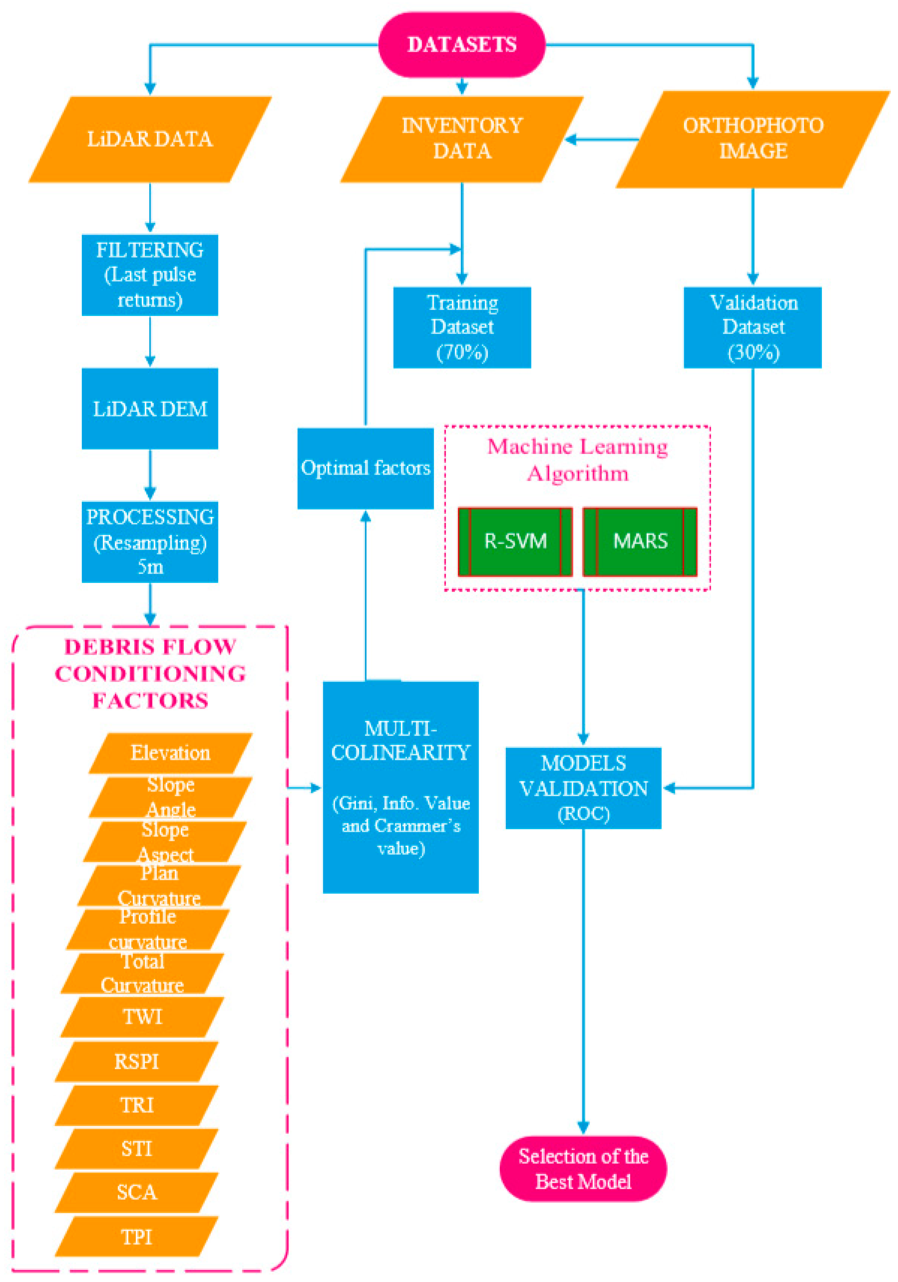
3. Materials and Methods

This study is conducted in Cameron Highlands, around the Ringlet area of Pahang in Peninsular Malaysia. Geographically, the study area lies within latitude 4°22′52″ N and 4°25′48″ N and longitude 101°22′30″ E to 101°23′30″ E (Figure 1) covering an area of about 25 km². This area is specifically chosen because of the frequent occurrences of landslides and slope instability that often results in debris-flow [47,79]. In terms of physical development, the study area experiences rapid developments, which have greatly altered the natural slope, potentially, putting the community living in downslope in danger. Generally, the topography of the Cameron Highlands area is underlain by rising and falling plateau ranging between the elevation of 1000 m and 1676 m a.s.l. [47]. The geological formation comprises of granites of various categories of megacrystic biotite and associated micro-granite (muscovite) [48,55,131] and meta-sediments comprising of slate, (Sedimentary rock) phyllite, limestone, sandstone and schist (metamorphic rock) [61]. The mean annual rainfall records range from 2500 to 3000 mm per annum. There are two raining seasons in the study area, which include; the September to December regime and the February to May regime but the peaks are recorded between March to May and November to December respectively. During the peak period, rainfall of between 88 mm to 100 mm in a single day usually triggers landslides [6,11,50,52,55]. When the local rainfall rate exceeds a distinctive intensity threshold, a runoff-generated debris flow may likely be initiated.

The occurrence of debris-flow events in this region of complex terrain is strongly induced by ubiquitous slopes-bed deposits of weathered-source grain sediments and weather system. Such as recurrent monsoon in the wet season is associated with thunderstorms that result in a locally intensive downpour; the recorded rainfall intensity is sufficient to trigger debris flow [17,20,26]. The risk presented by debris flow is dynamic and the threat related to a hydrological hazard could aggravate severe hazard in the near future due to modifying climate pattern in the tropical region that could change the precipitation system.

3.1. Data, Software and Techniques

The systematic procedures utilized to achieve the objectives of this research paper is summarized and illustrated in Figure 2. The datasets used in this study are ALS data, orthophoto and landslide-inventory data. The site was visited twice in 2017, first between 15th and 18th May and later from 19th to 23rd December. Twelve conditioning factors comprising of topographic and geomorphic parameters were derived from 5 m resolution LiDAR-derived DEM to model debris flow event using SVM and MAR Splines algorithms. The inventory data was assigned to the dependent variables while the conditioning factors represent the independent variables. Data processing was accomplished using different software packages these include Whitebox (open source software; https://www.whiteboxsoft.com), ArcGIS 10.6 (ESRI, Kuala Lumpur, Malaysia) software environment, LAStool in ArcGIS, Salford predictive Modeler 8.1 (Salford System, San Diego, CA USA), Statistica (StatSoft,Tulsa, OK, USA) and Waikato Environment for Knowledge Analysis (WEKA) version 3.9 (University of Waikato, Halmilton, New-Zealand).

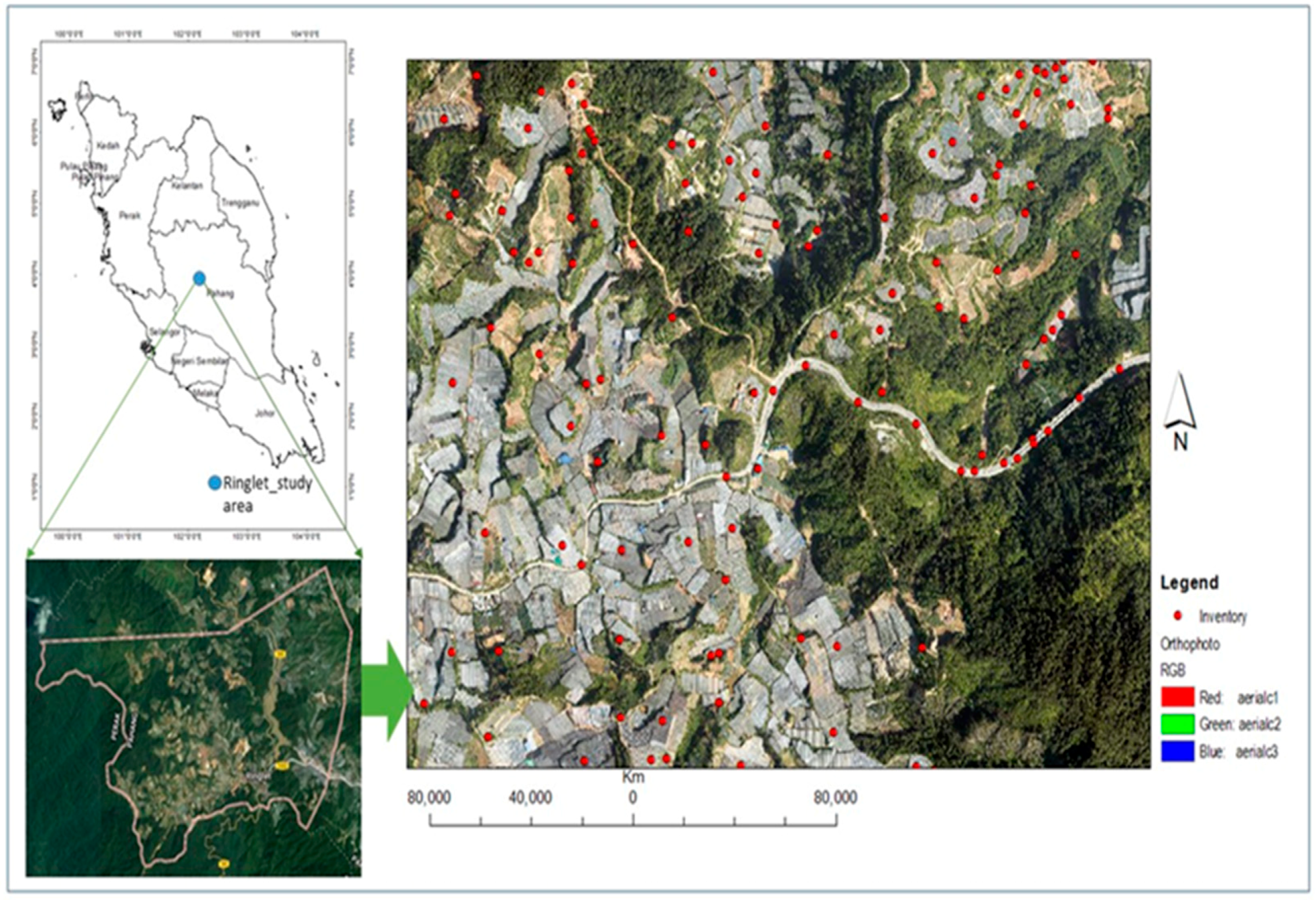
3.2. LiDAR Data Acquisition and Preparation

Airborne LiDAR data was acquired with discrete pulse return systems over Cameron Highlands in support to a regional scale assessment of landslides [11,52,132]. The LiDAR database comprises of pulses (beam), gathered in the scope of PBRC Project, 10th Malaysia Plan (RMKe-10), through Minerals and Geoscience Department Malaysia (JMG) in the year 2015. The LiDAR data was captured on the 15 January 2015 by a Malaysia-based Company, using a scanner aboard EC-120 Helicopter flown at an average altitude of 1676 m above m.s.l. The sensor was calibrated to sample at a 25,000 Hz pulse rate that yields ground point density of 8 points/m², 0.5 point spacing with a vertical accuracy of 15 cm on vegetated terrain and horizontal accuracy of 25 cm, fall within the acceptable threshold value for LiDAR processes in the area of land formations [133]. The acquisition exercise, footage stored a number of pulse-returns together with the first and last returns. In addition, an orthophoto image (0.09 × 0.09 m) was obtained during the LiDAR campaign, (Figure 1) in the scanned area using EOS5D Mark III camera with a focal length of 35 mm mounted on the aircraft. The camera has a horizontal and vertical resolution of 72 dpi, respectively, and exposure time of 1/2500 s.

The data pre-processing task commenced with a subset of the area of interest that covers a span of (5 km × 5 km) 25 km². LAStool of ArcGIS software package was utilized to filter out the other returns (vegetation and building) owed to their insignificance to this study. Keeping single LiDAR point cloud records size representing the ground surface, which is of interest to this research. First and last pulse return that made-up point cloud using morphological filtered approach to separate ground points from non-ground points, the latter represented the surface terrain morphology of the area and is selected for further analysis. The statistical reports have shown the LiDAR total point return is 3,998,752 where 2,848,914 (71.25%) was classified ground and 1,149,838 (28.75%) non-ground using LAStools add-in in ArcGIS software. The filtered ground LiDAR return points cloud dataset was interpolated into raster grids using a natural neighbor algorithm (NNA) via Triangulated Irregular Network (TIN) to produce a digital terrain model (DTM) of 5 m cell size utilizing the ArcGIS 10.6 software tool. Natural neighbor presented a ubiquitously smooth surface, but the position sample differs. This was chosen because of Baker and Coop [134], who stated that no technique of interpolation is superior to another when used for the interpolation of a DTM; thus they observed the model conservative and has the lowest error term. NNA adapted the principle of autocorrelation to the added inverse distance to a power function and related weights to the input samples in proportional areas to interpolate a value. Hence, the LiDAR data was used to produce a DEM of the study area at 5 m resolution. The LiDAR-derived DEM derived defines elevation of surface in term of planes, valleys and crests.

Obviously, no ideal grid resolution exists, but rather a range of suitable resolution [133] despite its significant role-plays in terrain efficiency mapping. Selection can be optimized to a certain level to satisfy both processing capabilities and representation of spatial variability. A grid resolution that optimally represents diverse terrain surface is required that is capable to reflect the majority of geomorphic attributes. A finer grid resolution can introduce local artefacts and slow down computation of terrain parameters. Kienzle [135,136] pointed a systematic overview of the effects of various grid resolutions on the reliability of terrain parameters suggesting fine grid resolutions from 5 m to 10 m. A LiDAR-derived DEM was generated at 5 m cell size signifying the LiDAR post spacing [135,137], exhibit hydromorphic structures used to generate the debris-flow conditioning factors.

Very high-resolution offers the prospect of the greater reliability of topographic features, which improves the identification of debris flow. The topographic reflectance dataset was utilized to generate primary and secondary terrain surface derivatives. Nevertheless, it could produce inherent issues related to the surface; generate anisotropic effects in the spatial resolution, generating artefacts. Pits in the DEM were filled to sieve out undulating artefacts to attain hydrological connectivity [138]. For computational efficiency, lessen prediction errors and increase model accuracy, the original DEM 0.5 m resolution data was spatially resampled to 5 m subsequently. According to Keijsers et al. [139], fine DEM resolution represents geomorphic and topographic configurations better than coarse DEM. Research has demonstrated the effects of different DEM resolutions on susceptibility mapping which indicates low DEMs resolution hinders true representation of terrain attributes because it smoothens local surface variability [139]. Based on the assumption that terrain conditions that initiate an event in the past will likely lead to a reoccurrence of such event in future, the LiDAR DEM was used to derive both the primary and secondary conditioning factors utilized in this investigation.

Statistical analysis of the debris flow inventory data and its conditioning factors were combined to formulate an independent input variable utilized to predict area susceptible to debris flow. This allows assessment of areas prone to debris flow for emergency planning. Researchers [70,71,77,85,99,107,115,140,141,142,143,144,145,146,147] have identified the relationships between earth movements and the conditioning factors associated with morphological, topographical, climatological, hydrological and human activities. However, the accuracy of debris-flow susceptibility mapping depends on the high quality of these input model factors data.

Unlike land use and climate variables which change rapidly over a short time, lithology and soil properties were all not considered as part of the conditioning factors in this study because they are assumed to be constant over a longer time scale [139]. In addition, rainfall data was exempted from the model because it is considerably uniform [47,148] over the small area.

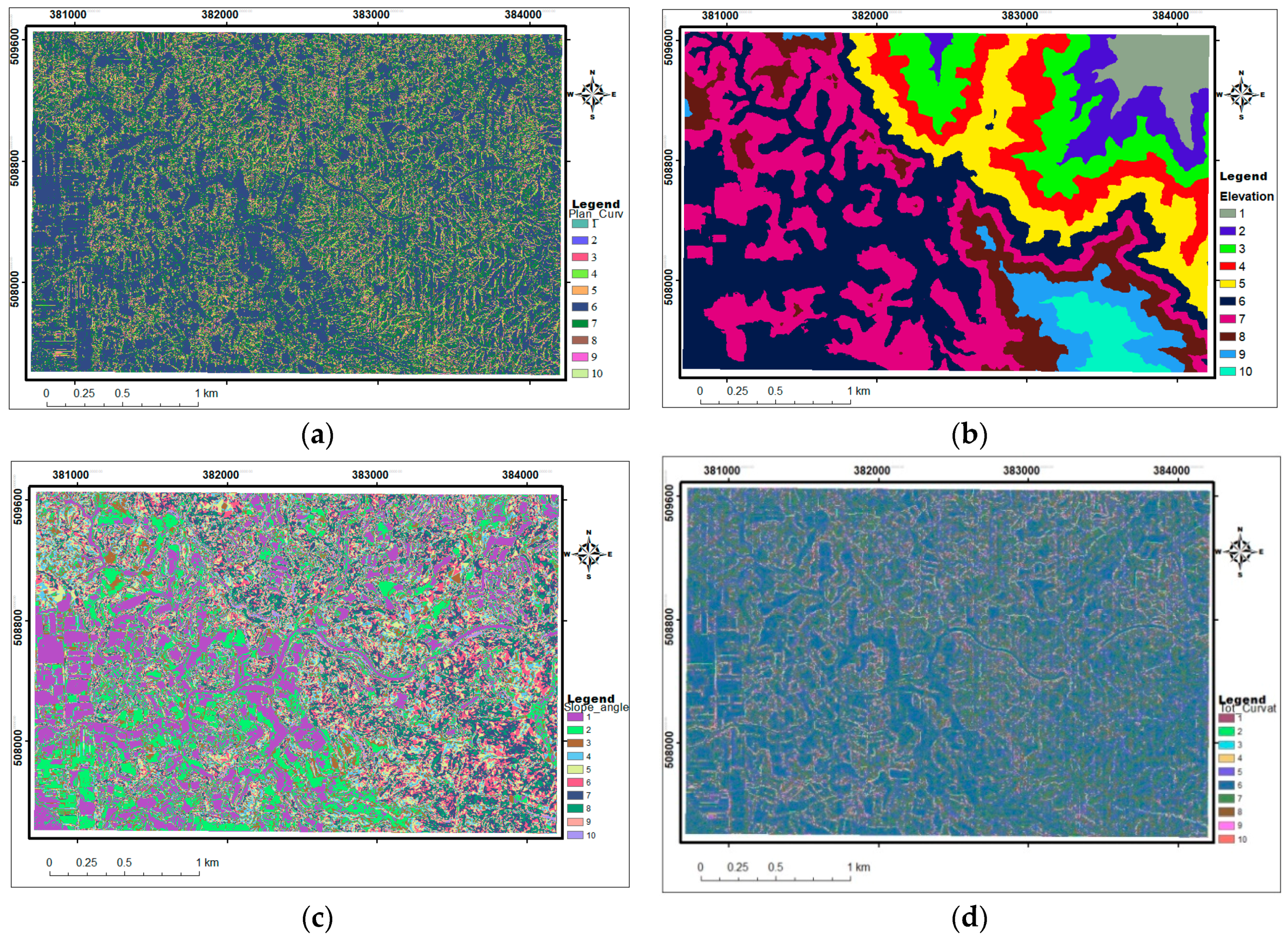
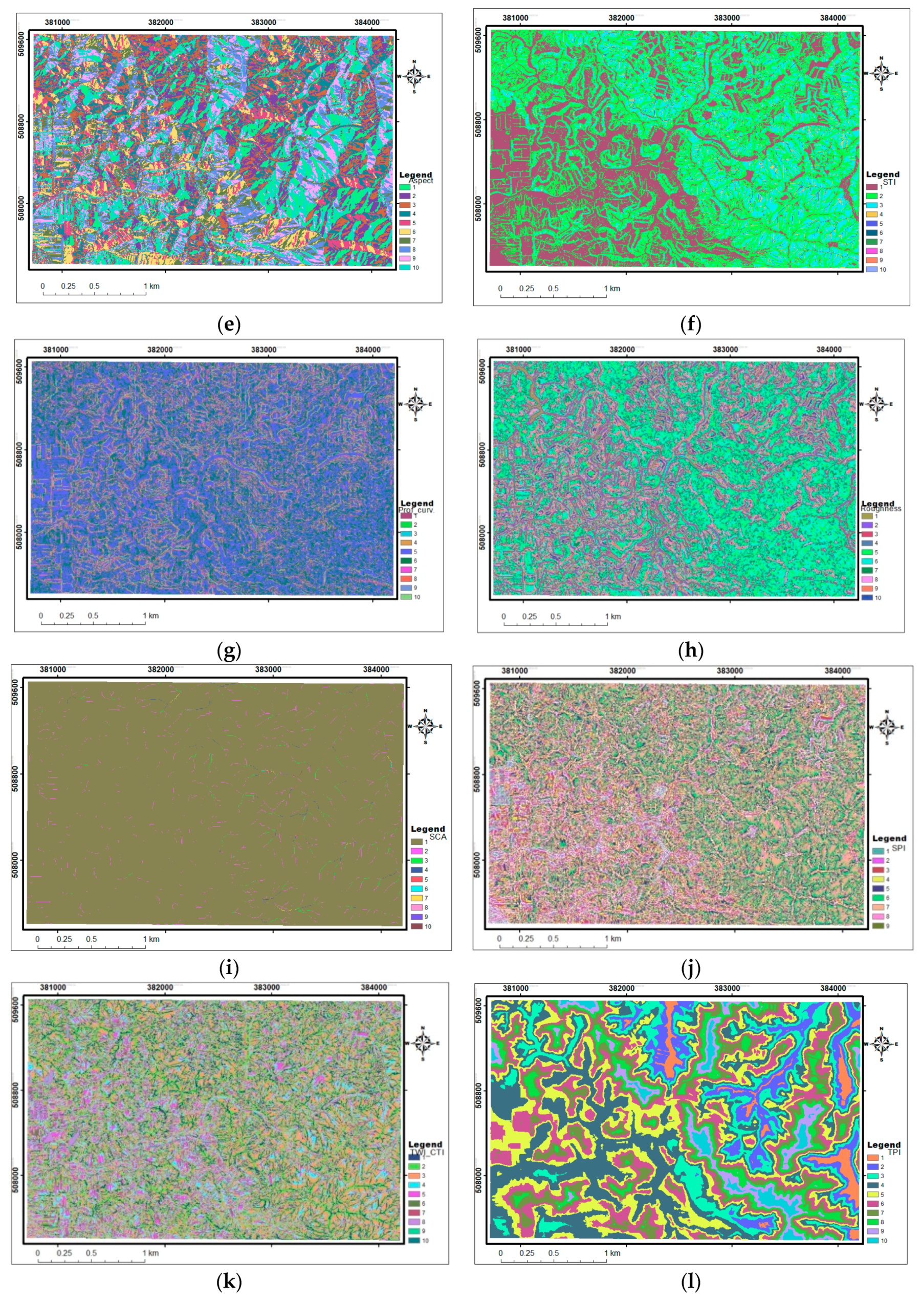
3.2.1. Derivation of Conditioning Factors

From, the thorough review of relevant literatures e.g., [38,60,115,149,150,151,152,153,154,155] twelve conditioning factors were selected and they were derived from the 2 m LiDAR DEM. These factors include; elevation (Figure 3a), plane curvature (Figure 3b), slope angle (Figure 3c), total curvature (Figure 3d), slope aspect (Figure 3e), Sediment Transport Index (STI) (Figure 3f), topographic profile curvature (Figure 3g), Topographic Roughness Index (TRI) (Figure 3h), flow accumulation/SCA (Figure 3i), Stream Power Index (SPI) (Figure 3j), Topographic Wetness Index (TWI) (Figure 3k), and Topographic Position Index (TPI) (Figure 3l). Generally, these variables are critical factors that control the occurrence and characteristics of mass movement and are widely adopted in geo-hazard modelling and assessments e.g., [7,23,38,39,42,48,81,89,156].

The elevation factor was extracted from LiDAR-derived DEM, which describes the general configuration of topography. It provides height value for each point on the surface relative to the reference datum, in this case, the mean sea level. Area of low altitude collects surface runoff rapidly from the slope angle, which allows debris deposition. High elevation initiated debris, flow on varying slopes and angle. The elevation was reclassified into five classes using the natural break classification scheme e.g., [85,87,98,110,122].

Burrough and McDonnell [157,158] recommended Horn slope algorithm to be more appropriate to estimate slope angle utilizing remotely sensed LiDAR-derived DEMs on rugged terrain; most importantly this algorithm is embedded in ArcGIS software (ESRI). Hence, slope angle was determined using the surface analysis tool of spatial analyst extension in ArcGIS 10.6 software environment, using elevation as input data. This factor is a measure of a tangential surface robustly potential proxy for debris flow occurrence. Thus, slope gradient or angle is one of the core conditioning factors in debris flow mapping and modelling [11,115,153,159,160] and terrain morphology. Geomorphometric applications are effectively determined on the local slope, calculated in the direction of undue rapid gradient from discrete pixel to its diagonal or adjoining grid cells. Different activities take place at different slope range, for example, at slope angles between 15° to 35°, debris flow initiation occurs [27,102,113,160,161,162,163,164] whereas run-out and deposition mechanism occurs at a slope between 15° to 20° and <9°, respectively [12].

Another slope related parameter is the slope aspect. Slope aspect was computed with surface analysis tool via spatial analyst tool of ArcGIS 10.6 software environment. The output was converted from radians to degrees [165], the values range from 359° to 1° representing a cardinality (direction) of the surface. While total curvature depicts the convex or concave terrain of neighboring grids, aspect describes the direction, which reveals a surrogate for exposure to the climatic factors. This shows the horizontal direction of the slope of a mountain orientation [77], which activates weathered and eroded materials to be transported down the slope in the study area. As earlier discussed, most of the past debris-flow hazards in the area were triggered by landslides (new or old) combined with heavy downpour (duration and intensity) during the monsoon seasons, with a defined direction of wind flow [166,167]. For example, during the monsoon season, the wind flows in Southeastern and Northeast directions [166], noteworthy to mention that the NE monsoon wind direction and movement bring out heavy rainfall while the SE monsoon is a dry wind. This heavy downpour triggers flooding and landslides. The slope aspect was expressed in a unit degree (0°–360°), oriented clockwise directions starting from the north position, The facet of the terrain defines the effects of weathering and the amount of rainfall in the area based on the level of the exposed surface [77].

TPI is a degree of association between the elevations of a principal position to the elevation of adjacent terrain (nearest neighbor), describing planes trench, and crests. TPI was estimated following the methods of [168,169] focal statistic tool was used with radius neighbourhood shape, maximum and minimum kernel window cell size (3 × 3) and (200 × 200) [165].

The flow accumulation parameter defined the drainage pattern of the study area. The parameter presents the cumulative amount of the number of pixels that logically drain into outlets [38]. The collective hydrologic flow value signifies the number of input pixels that contribute to the channel. To avoid misleading result, sinks in the DEM was filled before it is used to produce flow direction and subsequently flow accumulation.

Some debris-flow conditioning factors (Total, profile and plan curvatures) showed a positive relationship with flow accumulation. Profile curvature was estimated using the slope simplification approach revised by [170]. The profile curvature defines two distinct characteristics of the topography, convexity (positive) and concavity (negative) curvature of the terrain surface [77,142]. The concave curvature accumulate water and exhibit convergent of soil and hold deposit sometimes indicating positive pixel value on an image. While convex type of curvature does not hold any earth material and indicated by negative values and a flat surface with a zero value.

In addition to the parameters discussed above, a number of morphometric related indices were also calculated and included in the modelling. First is the Topographic Wetness Index (TWI) which involves the upslope contributing area, a slope raster and a number of geometric functions [171,172]. It is important to consider carefully the flow accumulation and slope because how they are calculated will strongly affect the TWI values. The value of each cell in the output raster is the value for the flow accumulation raster for the corresponding DEM. TWI is mathematically expressed as [90]:

$$TWI=ln\left[\frac{As}{tan\left(\beta \right) }\right]$$

(1)

where ln is the natural logarithm, As is the flow accumulation and $\beta$ is the slope angle.

Stream Power Index (SPI) as a hydrological factor is a product of catchment area and slope. SPI is used to identify suitable locations for soil conservation measures to reduce the effect of concentrated surface runoff [17,20,87]. It has a considerable impact on debris flow development which indicates the potential of a channel to cause erosion [77]. SPI is generated using Equation (2):

$$SPI=\frac{As}{tan\left(\beta \right)}$$

(2)

Sediment Transport Index (STI) accounts for the effect of topography on erosion. The 2D catchment area is used instead of the 1D slope length factor as in the Universal Soil Loss Equation:

$$STI={\left[\frac{As}{tan\left(\beta \right)}\right]}^{22.31/0.6}$$

(3)

$$Z_{i,n}=\frac{Z_i-\left(\frac{Z_{max}}{2}+\frac{Z_{min}}{2}\right)}{\frac{Z_{max-}{Z}_{min}}{2}}$$

(4)

where $Z_{i,n}$, represent the standardized value for $Z_i$, which signifies separate data point, $Z_{min}$ and $Z_{max}$ are the minimum and maximum in the datasets.

In data pre-preprocessing stage, we normalized individual datasets which transform the factor values to a common standard dimensional level. Because of the large variability observed in the range values of the processed conditioning factors. Each conditioning factors was normalized using (Equation (4)) that produced a pixel value ranging between 0 and 1, purposely to unify the conditioning factors, reduce high dimensionality differences in the modelling task [38], also allowing relative estimate and combination. Parameter values standardization can improve the model response, action that tends to stabilize variance, remove nonlinearity, and counter non-normality (SAS tutorial, 2019) and leads to better model fits.

3.2.2. Inventory Data for Model Training and Validation

Inventory data is vital to debris flow susceptibility analysis [6]. Based on existing historical records, 320-point locations of previous landslides/debris-flow events were obtained. The validity of the points was verified during the site visit using handheld GPS (GERMIN GPSMAP 78S) and the information provided by the local residents. Another 320 points representing non-debris-flow locations were randomly selected and combined with the inventory data for the modelling. The 640 points were labelled 1′s and 0′s for the classification process where the former indicates the presence of debris flow (in the past) and the latter represent the absence of debris flow [55]. For each point location, corresponding cell values of the normalized conditioning factor datasets were extracted using multi-values to point tools in ArcGIS 10.6 software and randomly split into training and test datasets using ratio 70% (448) to 30% (192) to develop and validate the resulting debris flow susceptibility model [38,55,78,104,111,112,115,154,173,174,175]. As earlier mentioned, MARS and SVR data mining techniques were adopted and these MLAs often accept binary classifications [107].

3.3. Debris Flow Susceptibility Modeling

Data pre-processing carried out to select relevant factors that have no influence on others but have strong relationships with the conditioning factors using the correlation approach and explores the factors accuracy metrics information value (IV) and Gini coefficient. Machine learning approaches of SVM and MARS are evaluators considered in debris flow susceptibility mapping.

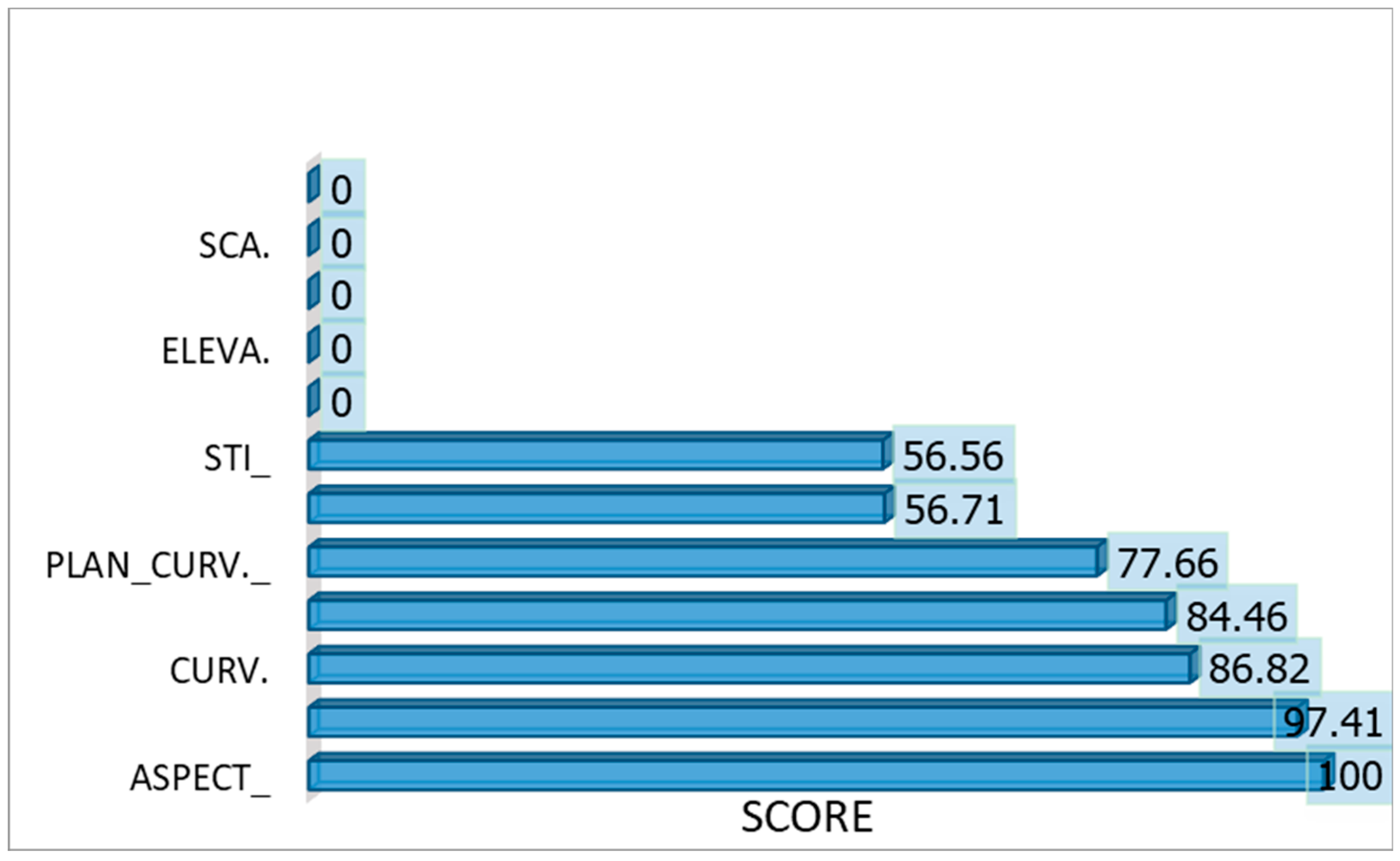
3.3.1. Debris Flow Conditioning Factor Selection

Several debris-flow conditioning factors have been experimented in many studies as input into data-mining algorithms. However, the selection process of the parameters is mostly not given proper consideration [176]. The inclusion of input parameters into modelling algorithms using the expert or a priori knowledge of the phenomenon could affect the quality of the model output [101,176]. The quality of a model’s output does not necessarily depend on the number of input parameters. Studies have established that the use of a huge number of factors practically increases the cost of data collection and processing time in addition to the possibility of generating misleading regression estimate [6]. Therefore, testing the credibility of input parameters by optimizing the conditioning factors is essential for reliable debris flow susceptibility modelling.

A very useful concept of variable selection in debris flow susceptibility model was done by optimizing information value (IV), utilizing Gini and Crammer values [42] under spearman correlation to examine the multi-collinearity effects in the predictor (input variables). This step allows identifying and subsequently discarding unrelated and out of range dataset, that usually affects the predictive accuracy of the model. It has been reported that a good feature subset is one that contains features highly correlated with the target, yet uncorrelated with each other [177]. IV (Equation (5)) is a statistical method for feature prediction that removes insignificant factors at 95% confidence level. The predictive power is expressed as such; <0.02 (bad predictor), 0.02 to 0.1 (weak predictor), 0.1 to 0.3 (moderate predictor), 0.3 to 0.5 (strong predictor) and >0.5 (Excellent predictor), which can also be expressed in percentage (%). Usually, variable all within moderate and strong predictive power are selected for model building. Optimum conditioning factors were selected using the IV, mathematically expressed as:

$$IV=\left[{\displaystyle \sum }_{i=1}^k\left(g_i-b_i\right) \times ln\left(\frac{g_i}{b_i}\right)\right] \times \%$$

(5)

where $k$ is the class size of individual conditioning factors, $g_i$ represent the distribution of good and $b_i$ denote the distribution of bad is the column-wise in percentage distribution of the total “debris flow” circumstances in the $ith$ case, $b_i$ is the percentage distribution of the total “no-debris flow” circumstances. The Gramer’s V statistic and Gini coefficient were calculated on individual conditioning factor. Gini coefficient is a measure of inequality in a given population and has an index value ranges from 0 (all factors are equal) to 1 (strength of affinity in an infinite variable). In addition, the Cramer’s V quantify the relationship amongst the conditioning factors and also, its value range from 0 (no relationship) to 1 (perfect relationship). The Cramer’s V is expressed as [92,116]:

$$V=\sqrt{\frac{x^2}{n \times min\left(w-1,k-1\right)}}$$

(6)

where $x^2$ is the Chi-square, $n$ is the number of entries existing in the dataset, $w$ is the size of the categorical dependent variable (i.e., “non-debris flow” and “debris flow” (=2) and $k$ is the size of factors present in the explanatory variables (i.e., the 12 debris flow conditioning factors).

Since the conditioning factors are non-parametric datasets, we adopted multiple regression using Spearman correlation method to further evaluate the relationships between the predictor and the conditioning factors (i.e., check for multicollinearity effects) purposely to indicate the level of insignificant relationship between the conditioning factors. Finally, all the conditioning factors that meet this hypothesis were selected and included in the modeling. Some of the input factors with a risen noise negatively contribute to the model building.

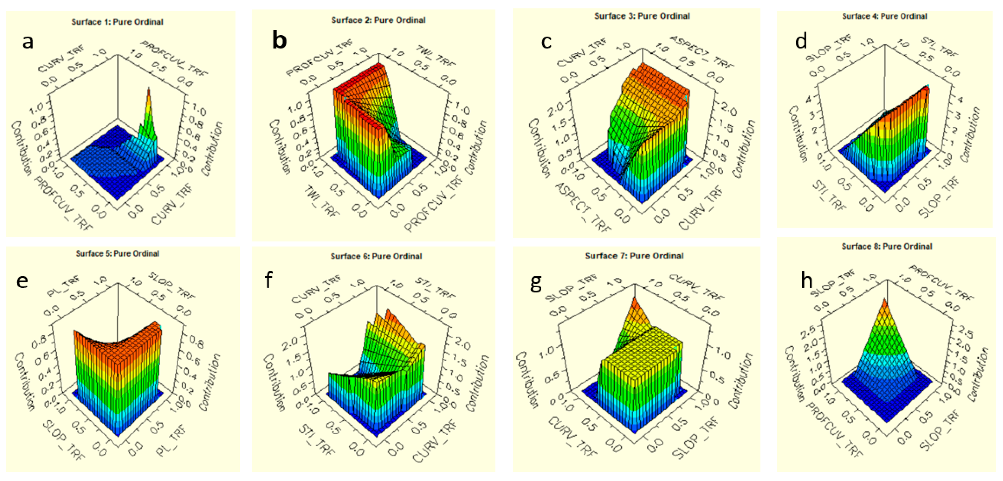
3.3.2. Multivariate Adaptive Regression Splines (MARS)

Multivariate Adaptive Splines (MARS) first put forward by [178] as one of the novel artificial intelligent approaches. MARS is a flexible, swift and accurate model for predicting continuous binary effects [116]. This approach integrates the mathematical structure of splines and the classical linear regression. The binary recursive splitting and instinctive search algorithm make it a model which is capable of predicting values from a given target variable (continuous and categorical) obtain from a dataset (independent variables). MARS employs basis function (BF) (Figure 3), a non-parametric and non-linear procedure that adopts discretization regression gradients at diverse intervals of the data frame for estimations. De-Andres et al. [116] noted that the recursive segregating approach that controls generalized additive modelling (GAM), classification and regression tree (CART) jointly motivates the MARS technique. The elasticity of the MARS method makes it possible to model correlations that embrace collaboration with limited parameters [116]. MARS is best at identifying optimal variable connections and transformations that expose intricate hidden data models successfully. It is also the capability of revealing a pattern that is rarely possible for other approaches to achieve [117].

The principal gain of the MARS model is that it clarifies the difficult in a nonlinear relationship between dependent and independent variables [126]. To do this, it approaches the underlying function through a set of piecewise functions, basic functions (BF), also known as Splines Polynomials [128,130]. The BF represents the information contained in one or more independent variables and was selected through a systematic process. The MARS model $f\left(x\right)$ is developed as a linear combination of BFs and the connections between them. MARS model is express in (Equation (7)) as:

$$y=f\left(x\right)={\beta }_0+{\displaystyle \sum }_{m=1}^M{\beta }_m{h}_m\left(x\right)$$

(7)

where y is the model expected value through a function $f\left(x\right)$ which could be disintegrated into an initial constant ${\beta }_0$, ${\beta }_m$ is the coefficient of the mth BF, $h_m\left(x\right)$ is a BF, and $n$ is the number of BFs in the model [88,179]. BFs are functions that proceed in either twofold modified formula as [90,122]:

$$\left(0,x-\alpha \right) or \left(0,\alpha -x\right)$$

(8)

where x is an independent (0 factors) variable and $\alpha$ is a constant, represent the node-to-node position. MARS utilizes truncated power functions as spline basis functions [180]. The Dual contiguous splines overlap at the knot to preserve the occurrence of the BF [122,127].

To generate the final MARS model, first, the forward stepwise algorithm (Equation (7)) was employed where a number of successive pairs of BFs of the model are added to obtain optimal performance [128,178]. This algorithm introduces complex over-fittings, which usually produce a poor estimate of the predicted results [116]. So, a second backward stepwise algorithm was applied to resolve the over-fitting by removing redundant BFs from the MARS model using Generalized Cross-Validation (GCV) (Equation (9)) [134]. The GCV limits the number of BFs to be included in the performance [128,130,179,181,182,183]:

$$GCV=\frac{\frac{1}{N}{{\displaystyle \sum }}_{i=1}^N{\left[y_i-\widehat{f}\left(x_i\right) \right]}^2}{{\left[1-\frac{C\left(B\right)}{N}\right]}^2}$$

(9)

where N is the number of data $\widehat{f}\left(x_i\right)$ is the projected value of the MARS model and $C\left(B\right)$ is a complexity penalty that rises with the number of basis functions ($BF)$ in the model. $C\left(B\right)$ is obtained from Equation (10):

$$C\left(B\right)=\left(B+1\right)+dB$$

(10)

where $d,$ a penalty is for each $BFs$ included in the model as a smoothing factor, and $B$ is the number of basis functions in Equation (7). The penalizing parameter $\left(d\right)$ signifies a cost BF optimization [128]. Increasing the number of d influences the size of the knotss while assigning higher values for d allows the use of less number of knots, smoother function estimates and small BFs [116]. The optimal value for the penalizing factor is between $2\le d\le 4$; however, Friedman [178] recommends 3. In the current work, a value of 3 is assigned to the penalty factor d similar to Zhang et al. [128]. In addition, the maximum interaction BFs level is limited to 10 for MARS approach with the optimal model size $M^{*}$ of 2 [130].

The MARS model was also used in the optimal feature selection process [26,81]. The contribution of each conditioning factors in the debris flow model was assessed in ANOVA. This procedure involves all the BFs related to both the individual factor and pairwise interaction aggregated separately through analysis of variance decomposition for statistical significance [178,183]. This was achieved by evaluating the coefficient of determination $R^2$, the coefficient of correlation r, mean average error (MAE), root mean squared error (RMSE), performance index $\rho$ and receiver operative curve (ROC). Finally, the performance rate and index are compared with SVM.

3.3.3. Support Vector Machine (SVM)

Support vector machines (SVM) is a supervised machine learning technique developed by Vladimir Vapnik and his colleagues in 1995 at AT&T Bell Laboratory [184]. SVM was originally developed for classification (C-SVM) and later adopted to solve regression (R-SVM) problems called support vector regression (R-SVM) [185,186]. The algorithm is based on statistical learning theory and structural risk minimization capable of addressing linear and non-linear multivariate regression problem [187]. SVM separates two opposite analogous hyperplanes and get the best separating distance between two vectors [106,127]. If the space between them is large, then the overall error of the classifier is reduced. The relationships among different categories of data in geosciences are mostly nonlinear. Therefore, it is recommended to adopt C-SVM also in nonlinear problems. Details on the SVM algorithm can be found in [102,105,188]. Mathematically, R-SVM is expressed as:

$$V=\frac{y_i\left(w.x_{i}b\right)}{\ge 1-{\xi }_i}$$

(11)

where, $w$ is the coefficient vector that defines the hyperplane positioning in the feature space, $b$ is the offset of the hyperplane from the source, and ${\xi }_i$ is the positive loose parameters [189,190]. To achieve optimal hyperplane, an optimization problem is resolved using the following mathematical equation [189,190]:

$$\begin{gathered} \mathrm{Minimize}{{\displaystyle \sum }}_{k=0}^n{\alpha }_i-\frac{1}{2}{{\displaystyle \sum }}_{i=1}^n{{\displaystyle \sum }}_{j=1}^n{\alpha }_i{\alpha }_j{y}_i{y}_i\left(x_i{x}_j\right) \\ \mathrm{Subject}\mathrm{to} {{\displaystyle \sum }}_{i=1}^n{\alpha }_i{y}_j=0, 0\le {\alpha }_i\le C, \end{gathered}$$

(12)

where ${\alpha }_{i }$ is the Lagrange multiplier, and $C$ is the model penalty. Thus, the decision function is demonstrated as follows:

$$g\left(x\right)=sign\left[{\displaystyle \sum }_{i=1}^n{y}_i{\alpha }_i{x}_i+b\right]$$

(13)

In an instance where the separating sample is nonlinear, the decision function is otherwise written as:

$$g\left(x\right)=sign\left[{\displaystyle \sum }_{i=1}^n{y}_i{\alpha }_{i}K\left(x_i,x_j\right)+b\right]$$

(14)

In this study, the initial data was converted to higher dimensional space by means of kernel functions (K). A number of kernel functions are available in SVM (polynomial, linear, sigmoid and radial basis) [190,191]. Prominently and most widely adopted kernel for mass movement applications, the radial basis function (RBF—Equation (15)) [78,101], is used in this study:

$$K\left(x_i,x_j\right)=exp\left(\frac{-\parallel x_i-x_j\parallel {}^2}{2{\delta }^2}\right)$$

(15)

where ${\delta }^2$ is the bandwidth of the RBF used to adjust the generalization, $x_i$ is the $i$-th support vector, and $x_j$ is the $j$-th support vector. The hyperplane function can be described as:

$$f\left(x\right)={\omega }^{T}x+b$$

(16)

where $\omega$ and $b$ are the coefficient.

The critical limitation conditions over an original optimization problem based on the SVR model explained as follows:

$$min\frac{1}{2}{\omega }^T\omega +C{{\displaystyle \sum }}_{i-1}^N({\xi }_i+{\xi }_i{}^{*})$$

(17)

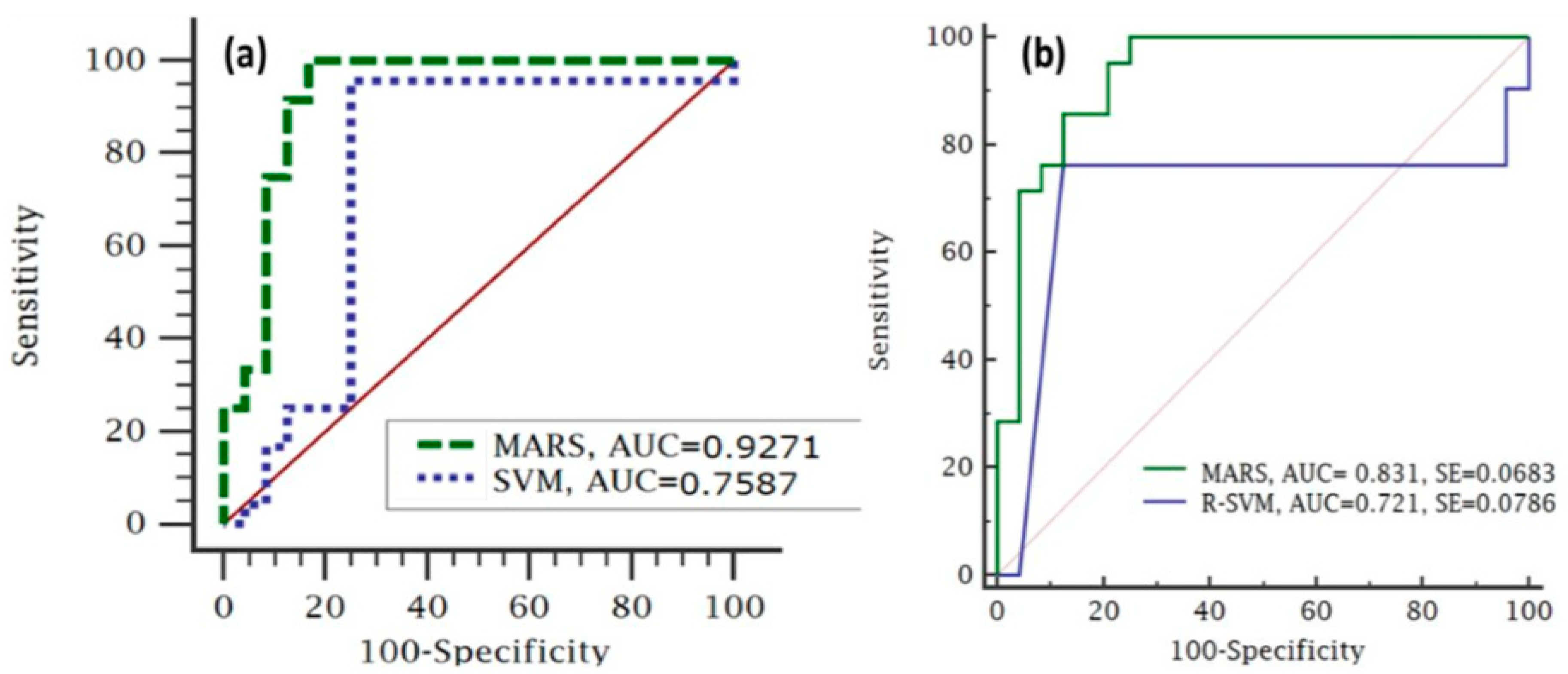
3.4. Model Validation and Evaluation

To evaluate the debris flow model performance, we used Receiver Operating Characteristics (ROC) sensitivity, specificity and accuracy evaluation techniques [6,104,125,192]. Area Under the Curve (AUC) values were used to compare the success and prediction rates [11,149,193,194]. ROC curve assesses the model’s capability to differentiate between the presence and absence of even represented in the specificity versus sensitivity measures (Figure 4). The ROC curve plots the false positive rate on the X-axis and true positive rate on the Y-axis. A good model has indicated with ROC curve fitted upper-left side and AUC value close to 1. Ordinal association between the model’s success rate is adjudged to be poor (0.5 to 0.6), average (0.6 to 0.7), good (0.7 to 0.8), very good (0.8 to 0.9) or excellent (0.9 to 1.0) [92,195].

Additionally, global performances of the model were evaluated to ascertain the power of the model in terms of prediction and capability strengths presented as success rate and prediction rate respectively; using the ROC/AUC (Equation (9)) [6,11,52,99,107,192,196]. The ROC curve is a dual scale plotted graph of Equation (18) against Equation (19). The curves are plotted on a Cartesian graph, calibrated on both positive axes (y-axis and x-axis) or vertical and horizontal lines with a scale units range from 0 to 1. It has been reported that the closer the curve toward the upper left of the vertical axis, the superior the model performance [99]. The quality of a model prediction or classification is demonstrated in a quantitative AUC value of categories scale as follows:

$$ROC=\frac{Sensitivity}{1-Specificity}$$

(18)

$$Specificity=\frac{TN}{TP+TN}$$

(19)

$$Sensitivity=\frac{TP}{TN+TP}$$

(20)

where TP is the True positive, TN denote the True negative.

4. Results

In this study, twelve conditioning factors (

Table 1. Features Selection measure of correlation and importance.

S/N	Variable	Information Value (IV)	Cramer’s V	Gini Coefficient	Important Score
1.	Slope Aspect	0.40	0.30	0.23	100
2.	Profile Curvature	0.28	0.26	0.07	97.41
3.	Total curvature	0.80	0.41	0.17	86.82
4.	Slope angle	0.62	0.37	0.06	84.46
5.	Plan curvature	0.57	0.36	0.15	77.66
6.	TWI	0.88	0.44	0.02	56.71
7.	STI	0.48	0.32	0.03	56.56
8.	TRI	0.68	0.47	0.06	0.00
9.	Elevation	0.61	0.36	0.33	0.00
10.	RSPI	0.94	0.45	0.03	0.00
11.	SCA	0.52	0.34	0.00	0.00
12.	TPI	0.49	0.30	0.01	0.00

) were prepared and optimized to predict area susceptibility to debris flow in Cameron Highlands. The multi-collinearity effects amongst the twelve conditioning factors and important contribution in the debris flow modelling using MARS rank are shown in Table 1. The Information Value (IV) indicated that profile curvature has an insignificant influence of about 28% on the other variables meaning that, it has no collinearity effect and strongly agreed by Cramer’s values (26%) and Gini coefficient (7%). The second level is the slope aspect with 40% IV, 30% Cramer’s Value and 23% Gini coefficient and is the most important variable in debris flow prediction with 100% MARS score function. RSPI was observed to have the highest multi-collinearity effect under IV of 94%. This is evidently shown on other evaluation metrics, which considered as a bad predictor and discarded from the advance analysis. The Cramer’s V relationship score reveals no significant correlation between each variable, which coincided with [176] this translate to no multi-collinearity effect present in the variables at 95% confidence level. In Gini coefficient, SCA, RSPI, TWI, STI and Profile Curvature demonstrated the presence of multicollinearity effects; this shows a certain level of disagreement, especially with Profile curvature. To satisfy the requirement for feature subset selection that is highly correlated with the target, there is a need for further evaluation on the training data [176].

Further analysis on the contribution of each variable through an optimization process with MARS algorithm indicates that only seven factors significantly influence the outcome. The measure of relative importance ranked in percentage is presented in (Figure 4). The most contributed or important conditioning factor in order of affinity is the slope aspect (100%) scored value and the least is STI (57%). Slope aspect contributes most to debris flow susceptibility with a measure of 100%; possibly because of the monsoon airstream bearing on the topography, which tends to make the high-slope side much more prone to debris flow initiation. Closely following the slope aspect is profile curvature, total curvature, slope angle and plan curvature with 97.41%, 86.82%, 84.46% and 77.66%, respectively. The other relative important variables are topographic wetness index and sediment transport index with 56.71% and 56.56% respectively. Similar feature subset selection was established by Jakob and Horton et al. [71,115]. The remaining five (TRI, elevation, RSPI, SCA and TPI) variables yielded zero or no contribution to the model building despite their theoretical contribution in mass movements modelling.

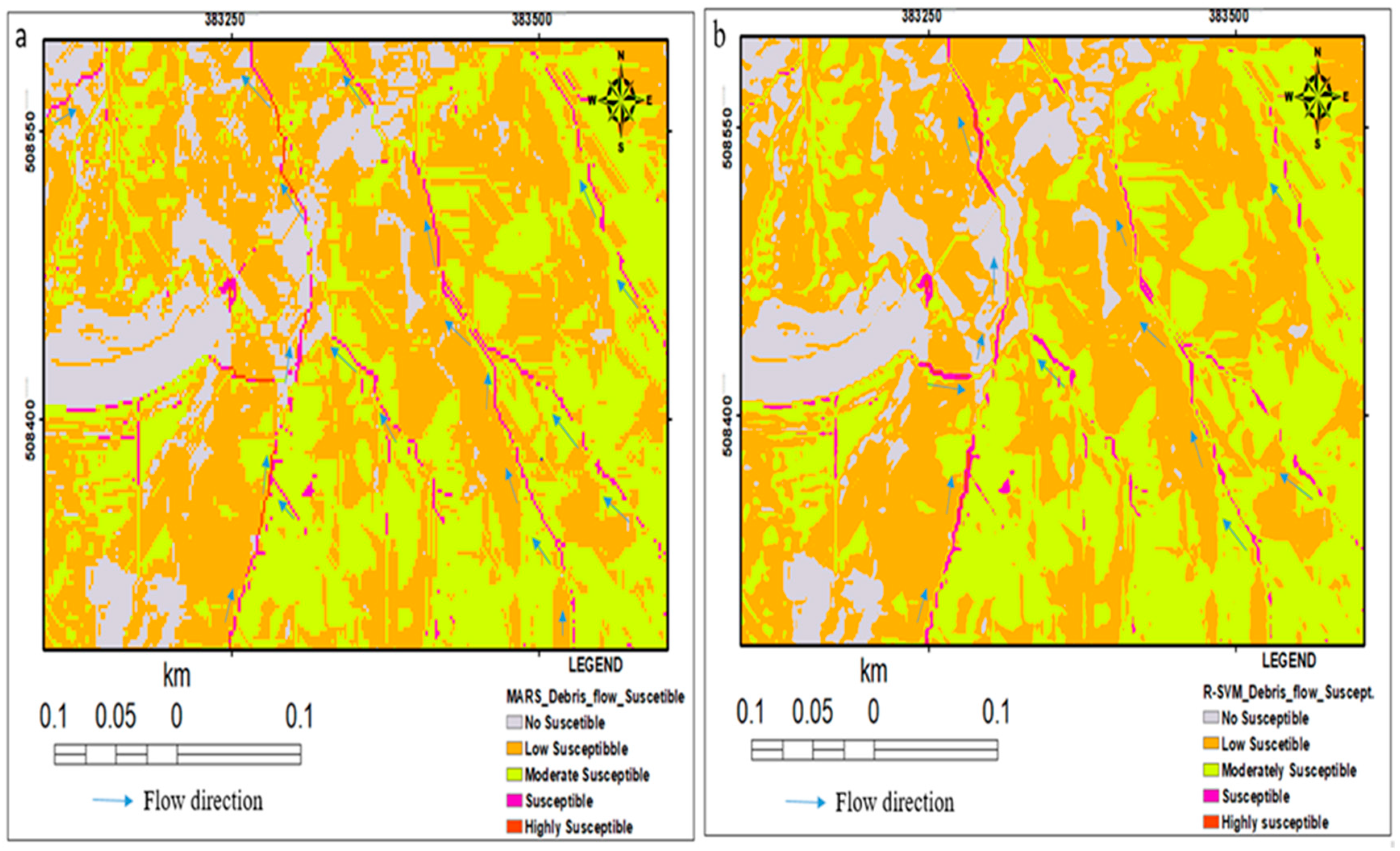
4.1. R-SVM for Debris Flow Susceptibility Mapping

R-SVM regression equation was used to generate a continuous debris flow susceptibility index map with a value range from 0.005 to 0.776. The quantitative model prediction index from the pixel values was classified into five classes using natural break classification scheme (0.005–0.155, 0.156–0.305, 0.306–0.455, 0.456–0.605, 0.606–0.776), this index received threshold digital number between 0 and 1 which signifies the possibility of debris flow pixel value in the catchment area. Afterwards, similar to the MARS result, both susceptibility indices maps were reclassified [6,78] into five classes (e.g., No susceptible, Low susceptible, Moderate susceptible, Susceptible and Highly susceptible) using natural break classification scheme and assigned qualitative importance of debris-flow susceptibility pixel value of to the classes (Figure 5a,b).

4.2. Debris Flow Susceptibility Mapping with MARS Approach

In this research, 15 BFs and knot locations generated and shown in

Table 2. BFs and knot locations.

No.	Relationship
1.	BF3 = max (0, CURV_TRF − 0.868835) × BF1;
2.	BF14 = max (0, CURV_TRF − 0.567935);
3.	BF27 = max (0, 0.852459 − TWI_TRF) × BF1;
4.	BF28 = max (0, ASPECT_TRF − 0.539546) × BF15;
5.	BF30 = max (0, STI_TRF − 0.5587) × BF24;
6.	BF40 = max (0, PROFCUV_TRF − 0.36921) × BF6;
7.	BF53 = max (0, PL_TRF − 0) × BF24;
8.	BF108 = max (0, STI_TRF − 0) × BF15;
9.	BF120 = max (0, CURV_TRF − 0) × BF18;
10.	BF136 = max (0, CURV_TRF − 0.554817);
11.	BF138 = max (0, CURV_TRF − 0.582064);
12.	BF140 = max (0, ASPECT_TRF − 2.98023 × 10−8) × BF139;
13.	BF146 = max (0, 0.977528 − SLOP_TRF) × BF138;
14.	BF147 = max (0, PROFCUV_TRF − 0.188011) × BF24;
15.	BF171 = max (0, STI_TRF − 0.0797712)

Notes: PROFCUV (Profile curvature), CURV_(Total Curvature), SLOP_(Slope), PLAN_CURV_ (Plane Curvature), TWI (Topographic Wetness Index), STI (Stream Transportation Index), Roughness (Surface Roughness Index), ELEVA (Elevation), SCA (Stream Catchment Index) and TPI (Topographic Position Index).

, BF used to describe individual interval of the conditioning factors. The debris flow susceptibility map generated by MARS model was produced using Equation (21) and rendered in Figure 5. This is executed in ArcGIS 10.6 software environment, MARSpline Salford Predictive Modeler (SPM) 8.1 software (https://www.salfordsystems.com); that generated the susceptibility map as shown in Figure 5.

Debris Flow (DF) = 1.17375 + 50.778 × BF3 − 59.505 × BF14 − 3.07208 × BF27 + 11.5545 × BF28 + 1.99699 × BF30 + 5.81348 × BF40 − 1.2703 × BF53 + 7.03378 × BF108 + 6.16987 × BF120 + 29.2086 × BF136 + 31.4915 × BF138 − 6.84261 × BF140 − 5.26128 × BF146 + 3.93846 × BF147 − 4.98071 × BF171.

(21)

The relationships between the explanatory variables and the contribution of the target variables are demonstrated on the response surface curves (Figure 6a–h). The figure explains the interaction between a pair of variables. Other contributions of the slope aspect, STI in describing the spatial distribution of debris flow shown in Figure 6c,d,f–h.

The seven optimal conditioning factors subset (Table 1) were utilized as input variables into MARS and R-SVM algorithm that produces the debris flow susceptibility model and generates a regression equation (Equation (20)) for the final debris flow susceptibility map (Figure 5). MARS model outputs susceptibility index value range is from 0.005 to 0.9999. This was further classified into five levels, which include Not Susceptible, Low Susceptible, Moderate Susceptible, Susceptible and Highly Susceptible using equal interval classification method (Figure 5).

4.3. Model Performance Evaluation

The general quantitatively produced performance accuracies of the debris flow model based on the ROC curve approach is shown in Figure 7a,b success rate and prediction rate by equating the two susceptibility maps with the debris flow training and validation datasets respectively. From the result, we observed that the MARS and R-SVM algorithms showed promising performance for debris flow susceptibility evaluation AUC between 0.72 and 0.92. The plot of the ROC curve Figure 7 and analysis of the indicators provided a quantitative appraisal of the model performance.

Performance evaluation of the two models using ROC curve indices shows that the MARS model transcended R-SVM model with AUC values of 0.9345 and 0.7587 respectively. Using the validation dataset, the model prediction rate produced AUC values of 0.831 and 0.721 for MARS and R-SVM models respectively. MARS have the highest success rate and prediction rates 0.935 and 0.832 respectively. The R-SVM model has the lowest measure of accuracy with a success rate of 0.7587 and prediction rate of 0.721.

5. Discussion

Studies such as [11,55,115,160,197,198,199] have confirmed the significance of slope aspect, profile curve, total curve and slope gradient to geo-hazard modelling. They observed the significant contribution of these conditioning factors (slope angle, plan curvature and flow accumulation) to debris flow initiation. In this study, STI, Roughness, Elevation, SPI, SCA and TPI were eliminated from advance analysis because they have zero scores and therefore lack predictive ability. Delmonaco et al. [200] pointed out that sediment availability, water input and slope gradient are the three main factors that directly or indirectly affect the possibility of debris flow initiation. Plan curvature, TWI and STI on the other hand, reveal the proportion of soil water content associated with the soil characteristics and denudations [198,201]. Nevertheless, the TWI is related more to debris flows than to landslides in low-order channels [124,162,202]. A high TWI value suggests the presence of surface depressions that prevent surface runoff and store surface water [48]. The factors excluded during the optimization process (elevation, SPI, surface roughness, SCA and TPI) reduces the objective function of the model (minimizing the error term). The excluded conditioning factors were considered redundancy was not involved in the prepared final modelling input independent variables; however, it does not mean they are not useful in the development of debris flow processes elsewhere. For instance, several studies have highlighted the role of elevation, SCA and SPI in debris flow and landslides in different environments [38,89,90,94,203].

The response curves relationship identified the contribution of profile curvature and TWI in debris flow potential modelling, this could be responsible for the hydrological effect on the debris flow catchment area. Thus, refers to an explanatory factor of fluid accumulation at a catchment area and signpost the tendency for debris flow propagation or run-out downslope due to the influence of gravitational forces [77]. Water permeation effects on soil strength divulge and reactivate the flow of debris from slope curvature of water to the lower values of profile curvature, which contributes most. From Figure 6e, slope gradient contributes intensively to the debris flow initiation to deposition at an angle range of 15° to 35° [11,115,173,204] and deposition zones ($\le$9°).

The quantitative susceptibility indices range from 0.005 to 0.9999 and 0.005 to 0.776 for MARS and R-SVM respectively. A pixel with 0 value indicates no possibility of debris flow while a pixel value of 1 indicates absolute debris flow of 100% possibility. The possible values need to be split into a specific number of classes that construct qualitative susceptibility maps to debris flow [105]. A meaningful decision can be derived from the maps via a nominal representation of the results. These were subjected to five qualitative classes the using natural break scheme, due to its adherence to a specific framework that manipulated the class into non-user defined categories [77]. The catchments were categorized into five areas of susceptibility levels; Not Susceptible, Low Susceptible, Moderate Susceptible, Susceptible and Highly Susceptible. The area in red colour denotes highly debris flow susceptibility. In contrast, visual susceptibility maps showed a glaring conflicting pixel class in Figure 5b, misclassification from highly susceptible class to moderate susceptible class. Drainages and second-order stream were predicted to be highly susceptible area to debris flow as shown in Figure 5a,b; for the purpose of mitigation measure, this zone is strongly not suitable for habitation, hence land-use developers should avoid it.

The model performance reveals MARS approach performing better than R-SVM [120,127,128,129]. The closer the ROC plot is to the upper left corner of the graph, the higher the overall accuracy [79,205,206]. The ROC curves are plotted on a Cartesian graph, calibrated on both positive axes (y-axis and x-axis) or on vertical and horizontal lines with a scale units range from 0 to 1. It has been reported that the closer the curve tends toward the upper left of the vertical axis of the graphs, the superior the model performance [99]. MARS success rate is toward the top right axis, which can term excellent with average prediction rate.

The competence of simple LiDAR-derived conditioning factor that offers promising and consistent debris flow susceptibility analysis have been demonstrated. This has similarly been proved in flood modelling [77]. However, the model’s efficiencies confirmed the significance of a feature subset selection and variables evaluation at the pre-processing stage of modelling. Although, exploration of advance feature subset selection and other machine learning algorithms could unveil different and better results.

6. Conclusions

This research demonstrated the use of laser scanning technology with MARS and R-SVM to develop models for the prediction of an area susceptible to debris flow, in the Ringlet region of the Cameron Highlands, which is affected by recurrent mass-movement related natural disasters. Triggered by anthropogenic and natural factors; utilized appropriate samples of training and test datasets to examine the interplays between the input factors (conditioning factors) and the dependent variable (debris flow inventory) for debris-flow susceptibility mapping. Geomorphometric and topographic elements generated from LiDAR-DEM (slope aspect, profile curvature, slope angle, total curvature plane curvature, TWI and STI) are observable factors that most contributed to debris flow prediction and susceptibility zones mapping in the Cameron Highlands. These parameters can be deemed suitable for a similar form of debris flow studies with minimal processing time and a high accuracy output.

The debris flow susceptibility maps revealed proficiencies of MARS and R-SVM algorithms with more than 72% AUC accuracy values, which yielded acceptable performance based on the success and prediction rates indicators. Interestingly, the MARS technique performed better with an accuracy difference of 2% in success rate and 1% prediction rates higher than R-SVM; this confirmed the efficacy of MARS application in debris flow prediction and detection of an area susceptible to debris flow. The pixel values generated from the debris flow susceptibility maps were classified into five using Jenk’s natural break classification scheme. The debris flow zone induced by the monsoon rain that twig by landslides will be greater than the events in the absence of landslides and the elevation of the debris source is developed toward the valley or mountain bottom.

Based on the accomplishments of the models used, this study also highlighted the significant contribution of MARS approach and LiDAR-derived DEM, suggesting for adoption in an area that has similar geographical settings. LiDAR provides high-resolution topographical data that represents the land surface more effectively. Therefore, the extracted topographic parameters from the laser scanning data permit realistic representation of the terrain configuration for debris flow in somewhat more reliable in susceptibility mappings.

Future investigation will explore the transferability of this model in a different environment using similar temporal LiDAR dataset on diverse topographic characteristics, which can improve model accuracy. In addition, advancement in feature subset selection is needed especially introducing metaheuristic nature-inspired optimization algorithm with Unmanned Aerial Vehicle (UAV) data may produce better results in future.

The outcome of this research paper will contribute to identifying the area susceptible to debris flow for the purpose of significant regional planning, land use and policies making processes. Such strategies can assist the government and decision-makers to reduce the risks associated with debris-flow disaster.

References

1. Iverson, R.M.; Reid, M.E.; Lahusen, R.G. Debris-Flow Mobilization from Landslides. Ann. Rev. Earth Planet. Sci. 1997, 25, 85–138. [Google Scholar] [CrossRef]
2. Iverson, R.M.; George, D.L. A depth-averaged debris-flow model that includes the effects of evolving dilatancy. I. Physical basis. Proc. R. Soc. A 2014. [Google Scholar] [CrossRef]
3. Iverson, R.M. Debris-Flow Hazards and Related Phenomena. In Debris-flow mechanics; Jakob, M., Hungr, O., Eds.; Springer: Berlin/Heidelberg, Germany, 2005; pp. 105–131. [Google Scholar]
4. Hürlimann, M.; McArdell, B.W.; Rickli, C. Field and laboratory analysis of the runout characteristics of hillslope debris flows in Switzerland. Geomorphology 2015, 232, 20–32. [Google Scholar] [CrossRef] [Green Version]
5. Melzner, S.; Lotter, M.; Linner, M.; Kociu, A. Regional analysis of slope instability processes along the southern border of the central Tauern Window (Eastern Alps). Austrian J. Earth Sci. 2015, 108, 93–110. [Google Scholar] [CrossRef]
6. Chen, W.; Peng, J.; Hong, H.; Shahabi, H.; Pradhan, B.; Liu, J.; Zhu, A.X.; Pei, X.; Duan, Z. Landslide susceptibility modelling using GIS-based machine learning techniques for Chongren County, Jiangxi Province, China. Sci. Total Environ. 2018, 626, 1121–1135. [Google Scholar] [CrossRef] [PubMed]
7. Chattoraj, S.L. Debris Flow Modelling and Risk Assessment of Selected Landslides from Uttarakhand-Case Studies Using Earth Observation Data. In Remote Sensing Techniques and GIS Applications in Earth and Environmental Studies; IGI: Hershey, PA, USA, 2017; pp. 111–121. [Google Scholar]
8. Xing, A.; Wang, G.; Li, B.; Jiang, Y.; Feng, Z.; Kamai, T. Long-runout mechanism and landsliding behaviour of large catastrophic landslide triggered by heavy rainfall in Guanling, Guizhou, China. Can. Geotech. J. 2015, 52, 971–981. [Google Scholar] [CrossRef]
9. Xing, A.; Yuan, X.; Xu, Q.; Zhao, Q.; Huang, H.; Cheng, Q. Characteristics and numerical runout modelling of a catastrophic rock avalanche triggered by the Wenchuan earthquake in the Wenjia valley, Mianzhu, Sichuan, China. Landslides 2017, 14, 83–98. [Google Scholar] [CrossRef]
10. Nakatani, K.; Hayami, S.; Mizuyama, T. Case study of debris flow disaster scenario caused by torrential rain on Kiyomizu-dera, Kyoto, Japan-using Hyper KANAKO system. J. Mt. Sci. 2016, 13, 193–203. [Google Scholar] [CrossRef]
11. Lay, U.S.; Pradhan, B. Identification of Debris Flow Initiation Zones Using Topographic Model and Airborne Laser Scanning Data. In Lecture Notes in Civil Engineering; Pradhan, B., Ed.; Springer Nature: Singerpore, 2019; pp. 915–940. [Google Scholar]
12. Schraml, K.; Thomschitz, B.; Mcardell, B.W.; Graf, C.; Kaitna, R. Modeling debris-flow runout patterns on two alpine fans with different dynamic simulation models. Nat. Hazards Earth Syst. Sci. 2015, 15, 1483–1492. [Google Scholar] [CrossRef] [Green Version]
13. Toyos, M.T.; Gunasekera, G.; Zanchetta, R.; Oppenheimer, G.; Sulpizio, C.; Favalli, R.; Pareschi, M. GIS-assisted modelling for debris flow hazard assessment based on the events of May 1998 in the area of Sarno, Southern Italy. Part II: Velocity and Dynamic Pressure. Earth Surf. Process. Landf. 2008, 33. [Google Scholar] [CrossRef]
14. Berti, M.; Genevois, R.; Simoni, A.; Tecca, P.R. Field observations of a debris flow event in the Dolomites. Geomorphology 1999, 29, 265–274. [Google Scholar] [CrossRef]
15. Berti, M.; Simoni, A. Experimental evidences and numerical modelling of debris flow initiated by channel runoff. Landslides 2005, 2, 171–182. [Google Scholar] [CrossRef]
16. Kean, J.W.; McCoy, S.W.; Tucker, G.E.; Staley, D.M.; Coe, J.A. Runoff-generated debris flows: Observations and modeling of surge initiation, magnitude, and frequency. J. Geophys. Res. Earth Surf. 2013, 118, 2190–2207. [Google Scholar] [CrossRef]
17. Gregoretti, C.; Degetto, M.; Bernard, M.; Boreggio, M. The Debris Flow Occurred at Ru Secco Creek, Venetian Dolomites, on 4 August 2015: Analysis of the Phenomenon, Its Characteristics and Reproduction by Models. Front. Earth Sci. 2018, 6, 1–20. [Google Scholar] [CrossRef]
18. Legg, N.T.; Meigs, A.J.; Grant, G.E.; Kennard, P. Geomorphology Debris flow initiation in proglacial gullies on Mount Rainier, Washington. Geomorphology 2014, 226, 249–260. [Google Scholar] [CrossRef]
19. Theule, J.I.; Liébault, F.; Loye, A.; Laigle, D.; Jaboyedoff, M. Sediment budget monitoring of debris-flow and bedload transport in the Manival Torrent, SE France. Nat. Hazards Earth Syst. Sci. 2012, 12, 731–749. [Google Scholar] [CrossRef] [Green Version]
20. Chen, M.L.; Liu, X.N.; Wang, X.K.; Zhao, T.; Zhou, J.W. Contribution of Excessive Supply of Solid Material to a Runoff-Generated Debris Flow during Its Routing along a Gully and Its Impact on the Downstream Village with Blockage Effects. Water 2019, 11, 169. [Google Scholar] [CrossRef]
21. Ma, C.; Deng, J.; Wang, R. Analysis of the triggering conditions and erosion of a runoff-triggered debris flow in Miyun County, Beijing, China. Landslides 2018, 15, 2475–2485. [Google Scholar] [CrossRef]
22. Armento, M.C.; Genevois, R.; Tecca, P.R. Comparison of numerical models of two debris flows in the Cortina d’ Ampezzo area, Dolomites, Italy. Landslides 2018, 5, 143–150. [Google Scholar] [CrossRef]
23. Meinhardt, M.; Fink, M.; Tünschel, H. Landslide susceptibility analysis in central Vietnam based on an incomplete landslide inventory: Comparison of a new method to calculate weighting factors by means of bivariate statistics. Geomorphology 2015, 234, 80–97. [Google Scholar] [CrossRef]
24. Cánovas, J.A.B.; Stoffel, M.; Corona, C.; Schraml, K.; Gobiet, A.; Tani, S.; Sinabell, F.; Fuchs, S.; Kaitna, R. Debris-flow risk analysis in a managed torrent based on a stochastic life-cycle performance. Sci. Total Environ. 2016, 557–558, 142–153. [Google Scholar] [CrossRef] [PubMed]
25. Dietrich, A.; Krautblatter, M. Evidence for enhanced debris-flow activity in the Northern Calcareous Alps since the 1980s (Plansee, Austria). Geomorphology 2015, 287, 144–158. [Google Scholar] [CrossRef]
26. Uzielli, M.; Rianna, G.; Ciervo, F.; Mercogliano, P.; Eidsvig, U.K. Temporal evolution of flow-like landslide hazard for a road infrastructure in the municipality of Nocera Inferiore (southern Italy) under the effect of climate change. Nat. Hazards Earth Syst. Sci. 2018, 18, 3019–3035. [Google Scholar] [CrossRef] [Green Version]
27. Chen, C.Y. Landslide and debris flow initiated characteristics after typhoon Morakot in Taiwan. Landslides 2016, 13, 153–164. [Google Scholar] [CrossRef]
28. Bel, C.; Liébault, F.; Navratil, O.; Eckert, N.; Bellot, H.; Fontaine, F.; Laigle, D. Rainfall control of debris-flow triggering in the Réal Torrent, Southern French Prealps. Geomorphology 2017, 291, 17–32. [Google Scholar] [CrossRef]
29. Underwood, S.J.; Schultz, M.D.; Berti, M.; Gregoretti, C.; Simoni, A.; Mote, T.; Saylor, A.M. Atmospheric circulation patterns, cloud-to-ground lightning, and locally intense convective rainfall associated with debris flow initiation in the Dolomite Alps of northeastern Italy. Nat. Hazards Earth Syst. Sci. 2016, 16, 509–528. [Google Scholar] [CrossRef] [Green Version]
30. Chen, J.C.; Jan, C.D.; Huang, W.S. Characteristics of rainfall triggering of debris flows in the Chenyulan watershed, Taiwan. Nat. Hazards Earth Syst. Sci. 2013, 13, 1015–1023. [Google Scholar] [CrossRef]
31. Floris, M.; D’Alpaos, A.; Squarzoni, C.; Genevois, R.; Marani, M. Recent changes in rainfall characteristics and their influence on thresholds for debris flow triggering in the Dolomitic area of Cortina d’Ampezzo, north-eastern Italian Alps. Nat. Hazards Earth Syst. Sci. 2010, 10, 571–580. [Google Scholar] [CrossRef]
32. Gregoretti, C.; Fontana, G.D. The triggering of debris flow due to channel-bed failure in some alpine headwater basins of the Dolomites: Analyses of critical runoff. Hydrol. Process. 2008, 22, 2248–2263. [Google Scholar] [CrossRef]
33. Lari, S.; Crosta, G.B.; Frattini, P.; Horton, P.; Jaboyedoff, M. Regional-scale debris flow risk assessment for an alpine valley. In Proceedings of the 5th International Conference on Debris-Flow Hazards Mitigation: Mechanics, Prediction, and Assessment, Padua, Italy, 14–17 June 2011; pp. 933–940. [Google Scholar]
34. Jamaludin, S.; Abdullah, C.H.; Kasim, N. Rainfall Intensity and Duration for Debris Flow Triggering in Peninsular Malaysia. In The Simulation of a Deep Large-Scale Landslide Near Aratozawa Dam Using a 3.0 MPa Undrained Dynamic Loading Ring Shear Apparatus; Springer: Berlin, Germnay, 2014; pp. 1–6. [Google Scholar]
35. Abdul Rahman, H. An Overview of Environmental Disaster in Malaysia and Preparedness Strategies. Iran. J. Publ. Health 2014, 43, 17–24. [Google Scholar]
36. Abdul, H.; Mapjabil, J. Landslides Disaster in Malaysia: An Overview. Health Environ. J. 2017, 8, 58–71. [Google Scholar]
37. Youssef, A.M.; Al-Kathery, M.; Pradhan, B.; El-Sahly, T. Debris flow impact assessment along the Al-Raith Road, Kingdom of Saudi Arabia, using remote sensing data and field investigations. Geomat. Nat. Hazards Risk 2016, 7, 620–638. [Google Scholar] [CrossRef]
38. Elkadiri, R.; Sultan, M.; Youssef, Y.M.; Elbayoumi, T.; Chase, R.; Bulkhi, A.B.; Al-Katheeri, M.M. A Remote Sensing-Based Approach for Debris-Flow Susceptibility Assessment Using Artificial Neural Networks and Logistic Regression Modeling. IEEE J. Sel. Top. Appl. Earth Obs. Remote Sens. 2014, 7, 4818–4835. [Google Scholar] [CrossRef]
39. Feizizadeh, B.; Aryal, J.; Roodposhti, T.B.M.S. Comparing GIS-based support vector machine kernel functions for landslide susceptibility mapping. Arab. J. Geosci. 2017, 10, 122. [Google Scholar] [CrossRef]
40. Scheidl, C.; Rickenmann, D.; Chiari, M. The use of airborne LiDAR data for the analysis of debris flow events in Switzerland. Nat. Hazards Earth Syst. Sci. 2008, 8, 1113–1127. [Google Scholar] [CrossRef] [Green Version]
41. Bull, J.M.; Miller, H.; Gravley, D.M.; Costello, D.; Hikuroa, D.C.H.; Dix, J.K. Assessing debris flows using LIDAR differencing: 18 May 2005 Matata event, New Zealand. Geomorphology 2010, 124, 75–84. [Google Scholar] [CrossRef] [Green Version]
42. Chen, W.; Pourghasemi, H.R.; Naghibi, S.A. Prioritization of landslide conditioning factors and its spatial modeling in Shangnan County, China using GIS-based data mining algorithms. Bull. Eng. Geol. Environ. 2018, 77, 611–629. [Google Scholar] [CrossRef]
43. Sookhan, S.; Eyles, N.; Putkinen, N. LiDAR-based volume assessment of the origin of the Wadena drumlin field, Minnesota, USA. Sediment. Geol. 2015, 338, 72–83. [Google Scholar] [CrossRef]
44. Neugirg, F.; Kaiser, A.; Huber, A.; Heckmann, T.; Schindewolf, M.; Schmidt, J.; Becht, M.; Haas, F. Using terrestrial LiDAR data to analyse morphodynamics on steep unvegetated slopes driven by different geomorphic processes. Catena 2016, 142, 269–280. [Google Scholar] [CrossRef]
45. Bhardwaj, A.; Sam, L.; Bhardwaj, A.; Martín-Torres, F.J. LiDAR remote sensing of the cryosphere: Present applications and future prospects. Remote Sens. Environ. 2016, 177, 125–143. [Google Scholar] [CrossRef]
46. Blasone, G.; Cavalli, M.; Marchi, L.; Cazorzi, F. Monitoring sediment source areas in a debris-flow catchment using terrestrial laser scanning. Catena 2014, 123, 23–36. [Google Scholar] [CrossRef]
47. Pradhan, B.; Lee, S. Regional landslide susceptibility analysis using back-propagation neural network model at Cameron Highland, Malaysia. Landslides 2010, 7, 13–30. [Google Scholar] [CrossRef]
48. Pradhan, B.; Sezer, E.A.; Gokceoglu, C.; Buchroithner, M.F. Landslide susceptibility mapping by neuro-fuzzy approach in a landslide-prone area (Cameron Highlands, Malaysia). IEEE Trans. Geosci. Remote Sens. 2010, 48, 4164–4177. [Google Scholar] [CrossRef]
49. Bui, D.T.; Tuan, T.A.; Klempe, H.; Pradhan, B.; Revhaug, I. Spatial prediction models for shallow landslide hazards: A comparative assessment of the efficacy of support vector machines, artificial neural networks, kernel logistic regression, and logistic model tree. Landslides 2016, 13, 361–378. [Google Scholar]
50. Pradhan, B.; Jebur, M.N.; Zulhaidi, H.; Shafri, M.; Tehrany, M.S. Data Fusion Technique Using Wavelet Transform and Taguchi Methods for Automatic Landslide Detection from Airborne Laser Scanning Data and QuickBird Satellite Imagery. IEEE Trans. Geosci. Remote Sens. 2016, 54, 1610–1622. [Google Scholar] [CrossRef]
51. Mojaddadi, H.; Pradhan, B.; Nampak, H.; Ahmad, N.; Ghazali, A.H.B. Ensemble machine-learning-based geospatial approach for flood risk assessment using multi-sensor remote-sensing data and GIS. Geom. Nat. Hazards Risk 2017, 8, 1080–1102. [Google Scholar] [CrossRef] [Green Version]
52. Kalantar, B.; Pradhan, B.; Naghibi, S.A.; Motevalli, A.; Mansor, S. Assessment of the effects of training data selection on the landslide susceptibility mapping: A comparison between support vector machine (SVM), logistic regression (LR) and artificial neural networks (ANN). Geom. Nat. Hazards Risk 2018, 5705, 1–21. [Google Scholar] [CrossRef]
53. Saez, J.L.; Corona, C.; Stoffel, M.; Gotteland, A.; Berger, F.; Liébault, F. Debris-flow activity in abandoned channels of the Manival torrent reconstructed with LiDAR and tree-ring data. Nat. Hazards Earth Syst. Sci. 2011, 11, 1247–1257. [Google Scholar] [CrossRef] [Green Version]
54. Yusoff, H.H.M.; Razak, K.A. Different Methods of Landslide Mapping in Cameron Highlands. Malays. J. Remote Sens. GIS 2015, 4, 85–91. [Google Scholar]
55. Pradhan, B.; Bahareh, K.; Waleed, M.A.; Bui, T.D. Debris Flow Susceptibility Assessment Using Airborne Laser Scanning Data. In Laser Scanning Applications in Landslide Assesement; Pradhan, B., Ed.; Springer: Berlin, Germany, 2017; pp. 85–113. [Google Scholar]
56. Gregoretti, C.; Degetto, M.; Boreggio, M. GIS-based cell model for simulating debris flow runout on a fan. J. Hydrol. 2016, 534, 326–340. [Google Scholar] [CrossRef]
57. Gregoretti, C.; Stancanelli, L.M.; Bernard, M.; Boreggio, M.; Degetto, M.; Lanzoni, S. Relevance of erosion processes when modelling in-channel gravel debris flows for efficient hazard assessment. J. Hydrol. 2019, 568, 575–591. [Google Scholar] [CrossRef]
58. Zhang, W.; Qing, J.C.; Yuke, W. Susceptibility analysis of large-scale debris flows based on combination weighting and extension methods. Nat. Hazards 2013, 66, 1073–1100. [Google Scholar] [CrossRef]
59. Naranjo, J.L.; van Westen, C.J.; Soeters, R. Evaluating the use of training areas in bivariate statistical landslide hazard analysis: A case study in Colombia. ITC J. 1994, 3, 292–300. [Google Scholar]
60. Ayalew, L.; Yamagishi, H. The application of GIS-based logistic regression for landslide susceptibility mapping in the Kakuda-Yahiko Mountains, Central Japan. Geomorphology 2005, 65, 15–31. [Google Scholar] [CrossRef]
61. Sezer, E.A.; Pradhan, B.; Gokceoglu, C. Manifestation of an adaptive neuro-fuzzy model on landslide susceptibility mapping: Klang valley, Malaysia. Expert Syst. Appl. 2011, 38, 8208–8219. [Google Scholar] [CrossRef]
62. Pfeifer, N.; Briese, C. Laser scanning—Principles and applications. In Proceedings of the GeoSiberia 2007—International Exhibition and Scientific Congress, Novosibirsk, Russia, 19–21 April 2017; pp. 1–20. [Google Scholar]
63. Lawrence, R. GPHY 429R Applied Remote Sensing, Lecture Note: LiDAR and Debris Flow Analysis; Montana State University: Bozeman, MT, USA, 2016. [Google Scholar]
64. Heritage, G.L.; Large, A.R.G. Laser Scanning for the Environmental Sciences; Wiley-Blackwell: Hoboken, NJ, USA, 2009. [Google Scholar]
65. Van Genderen, J.L. Airborne and Terrestrial Laser Scanning; CRC Press: Boca Raton, FL, USA, 2011. [Google Scholar]
66. Hetherington, D. Topographic Laser Ranging and Scanning: Principles and Processing; CRC Press: Boca Raton, FL, USA, 2010. [Google Scholar]
67. Polat, N.; Uysal, M.; Toprak, A.S. An investigation of DEM generation process based on LiDAR data filtering, decimation, and interpolation methods for an urban area. Measurement 2015, 75, 50–56. [Google Scholar] [CrossRef]
68. Slatton, K.C.; Carter, W.E.; Shrestha, R.L.; Dietrich, W. Airborne Laser Swath Mapping: Achieving the Resolution and Accuracy Required for Geosurficial Research. Geophys. Res. Lett. 2007, 34, 1–5. [Google Scholar] [CrossRef]
69. Chen, W.; Li, X.; Wang, Y.; Chen, G.; Liu, S. Forested landslide detection using LiDAR data and the random forest algorithm: A case study of the Three Gorges, China. Remote Sens. Environ. 2014, 152, 291–301. [Google Scholar] [CrossRef]
70. Jaboyedoff, M.; Oppikofer, T.; Abellán, A.; Derron, M.H.; Loye, A.; Metzger, R.; Pedrazzini, A. Use of LiDAR in landslide investigations: A review. Nat. Hazards 2012, 61, 5–28. [Google Scholar] [CrossRef]
71. Mathias, J. Debris-Flow Hazards and Related Phenomena; Jakob, M., Hungr, O., Eds.; Springer: Berlin, Germany, 2005; pp. 411–432. [Google Scholar]
72. Tobergte, D.R.; Curtis, S. Laser scanning for the environmental Sciences. J. Chem. Inf. Model. 2013, 53, 1689–1699. [Google Scholar]
73. Babcock, C.; Finley, A.O.; Cook, B.D.; Weiskittel, A.; Woodall, C.W. Modeling forest biomass and growth: Coupling long-term inventory and LiDAR data. Remote Sens. Environ. 2016, 182, 1–12. [Google Scholar] [CrossRef] [Green Version]
74. Minár, J.; Evans, I.S. Elementary forms for land surface segmentation: The theoretical basis of terrain analysis and geomorphological mapping. Geomorphology 2008, 95, 236–259. [Google Scholar] [CrossRef]
75. Cavalli, M.; Tarolli, P.; Marchi, L.; Fontana, G.D. The effectiveness of airborne LiDAR data in the recognition of channel-bed morphology. Catena 2008, 73, 249–260. [Google Scholar] [CrossRef]
76. Cavalli, M.; Marchi, L. Characterisation of the surface morphology of an alpine alluvial fan using airborne LiDAR. Nat. Hazards Earth Syst. Sci. 2008, 8, 323–333. [Google Scholar] [CrossRef]
77. Tehrany, M.S.; Jones, S.; Shabani, F. Identifying the essential flood conditioning factors for flood prone area mapping using machine learning techniques. Catena 2019, 175, 174–192. [Google Scholar] [CrossRef]
78. Hong, H.; Liu, J.; Zhu, A.X.; Shahabi, H.; Pham, B.P.; Chen, W.; Pradhan, B.; Bui, D.T. A novel hybrid integration model using support vector machines and random subspace for weather-triggered landslide susceptibility assessment in the Wuning area (China). Environ. Earth Sci. 2017, 76, 652. [Google Scholar] [CrossRef]
79. Shirzadi, A.; Tien, D.; Binh, B.; Pham, T.; Solaimani, K. Shallow landslide susceptibility assessment using a novel hybrid intelligence approach. Environ. Earth Sci. 2017, 76, 1–18. [Google Scholar] [CrossRef]
80. Rahmati, O.; Tahmasebipour, N.; Haghizadeh, A.; Pourghasemi, H.R.; Feizizadeh, B. Evaluation of different machine learning models for predicting and mapping the susceptibility of gully erosion. Geomorphology 2017, 298, 118–137. [Google Scholar] [CrossRef]
81. Chen, W.; Pourghasemi, H.R.; Panahi, M.; Kornejady, A.; Wang, J.; Xie, X.; Cao, S. Spatial prediction of landslide susceptibility using an adaptive neuro-fuzzy inference system combined with frequency ratio, generalized additive model, and support vector machine techniques. Geomorphology 2017, 297, 69–85. [Google Scholar] [CrossRef]
82. Leathwick, J.R.; Elith, J.; Hastie, T. Comparative performance of generalized additive models and multivariate adaptive regression splines for statistical modelling of species distributions. Ecol. Modell. 2006, 199, 188–196. [Google Scholar] [CrossRef]
83. Alavi, A.H.; Gandomi, A.H.; Lary, D.J. Progress of machine learning in geosciences: Preface. Geosci. Front. 2016, 7, 1–2. [Google Scholar] [CrossRef] [Green Version]
84. Carrara, A.; Cardinali, M.; Guzzetti, F.; Reichenbach, P. GIS Technology in Mapping Landslide Hazard. In Geographical Information Systems in Assessing Natural Hazards; Springer: Berlin, Germany, 1995; pp. 135–175. [Google Scholar]
85. Garosi, Y.; Sheklabadi, M.; Pourghasemi, H.R.; Besalatpour, A.A.; Conoscenti, C.; van Oost, K. Comparison of differences in resolution and sources of controlling factors for gully erosion susceptibility mapping. Geoderma 2018, 330, 65–78. [Google Scholar] [CrossRef]
86. Conoscenti, C.; Angileri, S.; Cappadonia, C.; Rotigliano, E.; Agnesi, V.; Märker, M. Gully erosion susceptibility assessment by means of GIS-based logistic regression: A case of Sicily (Italy). Geomorphology 2014, 204, 399–411. [Google Scholar] [CrossRef] [Green Version]
87. Conoscenti, C.; Angileri, S.E.; Rotigliano, E.; Schnabel, S. Using topographical attributes to evaluate gully erosion proneness (susceptibility) in two mediterranean basins: Advantages and limitations. Nat. Hazards 2015, 79, 291–314. [Google Scholar]
88. Gutiérrez, Á.G.; Contador, F.L.; Schnabel, S. Modeling Soil Properties at a Regional Scale Using GIS and Multivariate Adaptive Regression Splines. Available online: http://geomorphometry.org/system/file/GomezGutierrez2011bgeomorphometry.pdf. (accessed on 26 May 2019).
89. Paudel, U.; Oguchi, T.; Hayakawa, Y. Multi-Resolution Landslide Susceptibility Analysis Using a DEM and Random Forest. Int. J. Geosci. 2016, 7, 726–743. [Google Scholar] [CrossRef] [Green Version]
90. Zabihi, M.; Pourghasemi, H.R.; Pourtaghi, Z.S.; Behzadfar, M. GIS-based multivariate adaptive regression spline and random forest models for groundwater potential mapping in Iran. Environ. Earth Sci. 2016, 75, 665. [Google Scholar] [CrossRef]
91. Liu, K.; Ding, H.; Tang, G.; Song, C.; Liu, Y.; Jiang, L.; Zhao, B.; Gao, Y.; Ma, R. Large-scale mapping of gully-affected areas: An approach integrating Google Earth images and terrain skeleton information. Geomorphology 2018, 314, 13–26. [Google Scholar] [CrossRef]
92. Lary, D.J.; Alavi, A.H.; Gandomi, A.H.; Walker, A.L. Machine learning in geosciences and remote sensing. Geosci. Front. 2016, 7, 3–10. [Google Scholar] [CrossRef] [Green Version]
93. Nefeslioglu, H.A.; Gokceoglu, C.; Sonmez, H. An assessment on the use of logistic regression and artificial neural networks with different sampling strategies for the preparation of landslide susceptibility maps. Eng. Geol. 2008, 97, 171–191. [Google Scholar] [CrossRef]
94. Ahn, B.S.; Cho, S.S.; Kim, C.Y. Integrated methodology of rough set theory and artificial neural network for business failure prediction. Expert Syst. Appl. 2000, 18, 65–74. [Google Scholar] [CrossRef]
95. Choi, J.; Oh, H.J.; Lee, H.J.; Lee, C.; Lee, S. Combining landslide susceptibility maps obtained from frequency ratio, logistic regression, and artificial neural network models using ASTER images and GIS. Eng. Geol. 2012, 124, 12–23. [Google Scholar] [CrossRef]
96. Panja, P.; Velasco, R.; Pathak, M.; Deo, M. Application of artificial intelligence to forecast hydrocarbon production from shales. Mater. Today Commun. 2018, 4, 75–89. [Google Scholar] [CrossRef]
97. Chen, W.; Pourghasemi, H.R.; Zhao, Z. A GIS-based comparative study of Dempster-Shafer, logistic regression and artificial neural network models for landslide susceptibility mapping. Geocarto Int. 2017, 32, 367–385. [Google Scholar] [CrossRef]
98. Bui, D.T.; Pradhan, B.; Nampak, H.; Bui, Q.T.; Tran, Q.A.; Nguyen, Q.P. Hybrid artificial intelligence approach based on neural fuzzy inference model and metaheuristic optimization for flood susceptibilitgy modeling in a high-frequency tropical cyclone area using GIS. J. Hydrol. 2016, 540, 317–330. [Google Scholar]
99. Chen, W.; Reza, H.; Seyed, P.; Naghibi, A. A comparative study of landslide susceptibility maps produced using support vector machine with different kernel functions and entropy data mining models in China. Bull. Eng. Geol. Environ. 2018, 77, 647–664. [Google Scholar] [CrossRef]
100. Lohani, A.K.; Goel, N.K.; Bhatia, K.K.S. Improving real time flood forecasting using fuzzy inference system. J. Hydrol. 2014, 509, 25–41. [Google Scholar] [CrossRef]
101. Xu, C.; Xu, X.; Dai, F.; Saraf, A.K. Comparison of different models for susceptibility mapping of earthquake triggered landslides related with the 2008 Wenchuan earthquake in China. Comput. Geosci. 2012, 46, 317–329. [Google Scholar] [CrossRef]
102. Ma, Y.; Guo, G. Support Vector Machines Applications; Springer: Berlin, Germany, 2014; pp. 1–302. ISBN 9783319023. [Google Scholar]
103. Chen, W.; Ma, C.; Ma, L. Mining the customer credit using hybrid support vector machine technique. Expert Syst. Appl. 2009, 36, 7611–7616. [Google Scholar] [CrossRef]
104. Termeh, S.V.R.; Kornejady, A.; Pourghasemi, H.R.; Keesstra, S. Flood susceptibility mapping using novel ensembles of adaptive neuro fuzzy inference system and metaheuristic algorithms. Sci. Total Environ. 2018, 615, 438–451. [Google Scholar] [CrossRef]
105. Pradhan, B. A comparative study on the predictive ability of the decision tree, support vector machine and neuro-fuzzy models in landslide susceptibility mapping using GIS. Comput. Geosci. 2013, 51, 350–365. [Google Scholar] [CrossRef]
106. Hamadeh, N.; Karouni, A.; Daya, B. Predicting Forest Fire Hazards Using Data Mining Techniques: Decision Tree and Neural Networks. Adv. Mater. Res. 2014, 1051, 466–470. [Google Scholar] [CrossRef]
107. Bui, D.T.; Panahi, M.; Shahabi, H.; Singh, V.P.; Shirzadi, A.; Chapi, K.; Khosravi, K.; Chen, W.; Panahi, S.; Li, S.; et al. Novel Hybrid Evolutionary Algorithms for Spatial Prediction of Floods. Sci. Rep. 2018, 8, 15364. [Google Scholar] [CrossRef]
108. Rodriguez-Galiano, V.; Sanchez-Castillo, M.; Chica-Rivas, M. Machine learning predictive models for mineral prospectivity: An evaluation of neural networks, random forest, regression trees and support vector machines. Ore Geol. Rev. 2015, 71, 804–818. [Google Scholar] [CrossRef]
109. Wu, J.; Chen, G.Q.; Zheng, L.; Zhang, Y.B. GIS-based numerical modelling of debris flow motion across three-dimensional terrain. J. Mt. Sci. 2013, 10, 522–531. [Google Scholar] [CrossRef] [Green Version]
110. Yalcin, A. GIS-based landslide susceptibility mapping using analytical hierarchy process and bivariate statistics in Ardesen (Turkey): Comparisons of results and confirmations. Catena 2008, 72, 1–12. [Google Scholar] [CrossRef]
111. Shi, M.; Chen, J.; Sun, D.; Zhang, X. Assessing debris flow susceptibility in mountainous area of Beijing, China using a combination weighting and an improved fuzzy C-means algorithm. Chem. Eng. Trans. 2015, 46, 697–702. [Google Scholar]
112. Chen, X.; Chen, H.; You, Y.; Liu, J. Susceptibility assessment of debris flows using the analytic hierarchy process method—A case study in Subao river valley, China. J. Rock Mech. Geotech. Eng. 2015, 7, 404–410. [Google Scholar] [CrossRef]
113. Pradhan, B.; Abu-Bakar, S.B. Debris Flow Source Identification in Tropical Dense Forest Using Airborne Laser Scanning Data and Flow-R Model. In Laser Scanning Applications in Landslide Assessment; Pradhan, B., Ed.; Springer: Basel, Switzerland, 2017; pp. 1–359. [Google Scholar]
114. Fischer, L.; Rubensdotter, L.; Sletten, K.; Stalsberg, K.; Horton, P.; Jaboyedoff, M. Debris flow modeling for susceptibility mapping at regional to national scale in Norway. In Proceedings of the 11th International and 2nd North American Symposium on Landslides, Banff, AB, Canada, 3–8 June 2012; pp. 723–729. [Google Scholar]
115. Horton, P.; Jaboyedoff, M.; Rudaz, B.; Zimmermann, M. Flow-R, a model for susceptibility mapping of debris flows and other gravitational hazards at a regional scale. Nat. Hazards Earth Syst. Sci. 2013, 13, 869–885. [Google Scholar] [CrossRef] [Green Version]
116. de Andrés, J.; Lorca, P.; Juez, F.J.D.; Sánchez-Lasheras, F. Bankruptcy forecasting: A hybrid approach using fuzzy c-means clustering and multivariate adaptive regression splines (MARS). Expert Syst. Appl. 2011, 38, 1866–1875. [Google Scholar] [CrossRef]
117. Lee, S.; Talib, J.A. Probabilistic landslide susceptibility and factor effect analysis. Environ. Geol. 2005, 47, 982–990. [Google Scholar] [CrossRef]
118. Kim, G.; Yune, C.Y.; Paik, J.; Lee, S.W. Analysis of debris flow behavior using airborne LiDAR and image data. Int. Arch. Photogramm. Remote Sens. Spat. Inf. Sci. 2016, 41, 85–88. [Google Scholar] [CrossRef]
119. Park, D.W.; Lee, S.R.; Vasu, N.N.; Kang, S.H.; Park, J.Y. Coupled model for simulation of landslides and debris flows at local scale. Nat. Hazards 2016, 81, 1653–1682. [Google Scholar] [CrossRef]
120. Zhang, W.G.; Goh, A.T.C. Multivariate adaptive regression splines for analysis of geotechnical engineering systems. Comput. Geotech. 2013, 48, 82–95. [Google Scholar] [CrossRef]
121. Crino, S.; Brown, D.E. Global optimization with multivariate adaptive regression splines. IEEE Trans. Syst. Man Cybern. Part B Cybern. 2007, 37, 333–340. [Google Scholar] [CrossRef]
122. Park, S.; Hamm, S.; Jeon, H.; Kim, J. Evaluation of Logistic Regression and Multivariate Adaptive Regression Spline Models for Groundwater Potential Mapping Using R and GIS. Sustainability 2017, 9, 1157. [Google Scholar] [CrossRef]
123. Deo, R.C.; Kisi, O.; Singh, V.P. Drought forecasting in eastern Australia using multivariate adaptive regression spline, least square support vector machine and M5Tree model. Atmos. Res. 2017, 184, 149–175. [Google Scholar] [CrossRef]
124. Conoscenti, C.; Ciaccio, M.; Caraballo-arias, N.A.; Gómez-gutiérrez, Á.; Rotigliano, E.; Agnesi, V. Geomorphology Assessment of susceptibility to earth-flow landslide using logistic regression and multivariate adaptive regression splines: A case of the Belice River basin (western Sicily, Italy). Geomorphology 2015, 242, 49–64. [Google Scholar] [CrossRef]
125. Roy, S.S.; Roy, R.; Balas, V.E. Estimating heating load in buildings using multivariate adaptive regression splines, extreme learning machine, a hybrid model of MARS and ELM. Renew. Sustain. Energy Rev. 2018, 82, 4256–4268. [Google Scholar]
126. Gutiérrez, Á.G.; Schnabel, S.; Contador, J.F.L. Using and comparing two nonparametric methods (CART and MARS) to model the potential distribution of gullies. Ecol. Model. 2009, 220, 3630–3637. [Google Scholar] [CrossRef]
127. Kisi, O.; Parmar, K.S. Application of least square support vector machine and multivariate adaptive regression spline models in long term prediction of river water pollution. J. Hydrol. 2016, 534, 104–112. [Google Scholar] [CrossRef]
128. Zhang, W.; Goh, A.T.C.; Zhang, Y. Multivariate Adaptive Regression Splines Application for Multivariate Geotechnical Problems with Big Data. Geotech. Geol. Eng. 2016, 34, 193–204. [Google Scholar] [CrossRef]
129. Zhang, W.; Goh, A.T.C. Multivariate adaptive regression splines and neural network models for prediction of pile drivability. Geosci. Front. 2016, 7, 45–52. [Google Scholar] [CrossRef] [Green Version]
130. Zhang, W.; Zhang, Y.; Goh, A.T.C. Multivariate adaptive regression splines for inverse analysis of soil and wall properties in braced excavation. Tunn. Undergr. Sp. Technol. 2017, 64, 24–33. [Google Scholar] [CrossRef]
131. Id, S.; Count, W. Geomorphometric Analysis of Landform Pattern Using Topographic Position and ASTER GDEM by Jibrin Gambo. In Proceedings of the Global Civil Engineering Conference, Kuala Lumpur, Malaysia, 25–28 July 2017. [Google Scholar]
132. Nouwakpo, S.K.; Weltz, M.A.; Green, C.H.M.; Arslan, A. Combining 3D data and traditional soil erosion assessment techniques to study the effect of a vegetation cover gradient on hillslope runoff and soil erosion in a semi-arid catchment. Catena 2018, 170, 129–140. [Google Scholar] [CrossRef]
133. Vianello, A.; Cavalli, M.; Tarolli, P. LiDAR-derived slopes for headwater channel network analysis. Catena 2009, 76, 97–106. [Google Scholar] [CrossRef]
134. Bater, C.W.; Coops, N.C. Evaluating error associated with lidar-derived DEM interpolation. Comput. Geosci. 2009, 35, 289–300. [Google Scholar] [CrossRef]
135. Hengl, T. Finding the right pixel size. Comput. Geosci. 2006, 32, 1283–1298. [Google Scholar] [CrossRef]
136. Kienzle, S. The Effect of DEM Raster Resolution on First Order, Second Order and Compound Terrain Derivatives. Trans. GIS 2004, 8, 83–111. [Google Scholar] [CrossRef]
137. Hill, R.A.; Hinsley, S.A. Airborne lidar for woodland habitat quality monitoring: Exploring the significance of lidar data characteristics when modelling organism-habitat relationships. Remote Sens. 2015, 7, 3446–3466. [Google Scholar] [CrossRef]
138. Hengl, T. A Practical Guide to Geostatistical Mapping; Open Access: Hague, The Netherlands, 2009. [Google Scholar]
139. Keijsers, J.G.S.; Schoorl, J.M.; Chang, K.T.; Chiang, S.H.; Claessens, L.; Veldkamp, A. Calibration and resolution effects on model performance for predicting shallow landslide locations in Taiwan. Geomorphology 2011, 133, 168–177. [Google Scholar] [CrossRef]
140. Fangqiang, W.; Yu, Z.; Kaiheng, H.; Kechang, G. Model and method of debris flow risk zoning based on momentum analysis. Wuhan Univ. J. Nat. Sci. 2006, 11, 835–839. [Google Scholar] [CrossRef]
141. Jain, I.; Kumar, V.; Jain, R. Correlation feature selection based improved-Binary Particle Swarm Optimization for gene selection and cancer classification. Appl. Soft Comput. J. 2018, 62, 203–215. [Google Scholar] [CrossRef]
142. Zabihi, M.; Mirchooli, F.; Motevalli, A.; Darvishan, A.K.; Pourghasemi, H.R.; Zakeri, M.A.; Sadighi, F. Spatial modelling of gully erosion in Mazandaran Province, northern Iran. Catena 2018, 161, 1–13. [Google Scholar] [CrossRef]
143. Staley, D.M.; Wasklewicz, T.A.; Blaszczynski, J.S. Surficial patterns of debris flow deposition on alluvial fans in Death Valley, CA using airborne laser swath mapping data. Geomorphology 2006, 74, 152–163. [Google Scholar] [CrossRef]
144. Federico, F.; Cesali, C. An energy-based approach to predict debris flow mobility and analyze empirical relationships. Can. Geotech. J. 2015, 52, 2113–2133. [Google Scholar] [CrossRef] [Green Version]
145. Pradhan, A.M.S.; Kang, H.-S.; Lee, S.; Kim, Y.-T. Spatial model integration for shallow landslide susceptibility and its runout using a GIS-based approach in Yongin, Korea. Geocarto Int. 2016, 6049, 1–55. [Google Scholar] [CrossRef]
146. Casas, A.; Riaño, D.; Greenberg, J.; Ustin, S. Assessing levee stability with geometric parameters derived from airborne LiDAR. Remote Sens. Environ. 2012, 117, 281–288. [Google Scholar] [CrossRef]
147. Conway, S.J.; Decaulne, A.; Balme, M.R.; Murray, J.B.; Towner, M.C. A new approach to estimating hazard posed by debris flows in the Westfjords of Iceland. Geomorphology 2010, 114, 556–572. [Google Scholar] [CrossRef] [Green Version]
148. Pradhan, B.; Chaudhari, A.; Adinarayana, J.; Buchroithner, M.F. Soil erosion assessment and its correlation with landslide events using remote sensing data and GIS: A case study at Penang Island, Malaysia. Environ. Monit. Assess. 2012, 184, 715–727. [Google Scholar] [CrossRef]
149. Kailey, P. Debris Flows in New Zealand Alpine Catchments. Ph.D. Thesis, University of Canterbury, Christchurch, New Zealand, February 2013. [Google Scholar]
150. Frey, H.; Huggel, C.; Bühler, Y.; Buis, D.; Burga, M.D.; Choquevilca, W.; Fernandez, F.; Hernández, J.G.; Giráldez, C.; Loarte, E.; et al. A robust debris-flow and GLOF risk management strategy for a data-scarce catchment in Santa Teresa, Peru. Landslides 2016, 13, 1493–1507. [Google Scholar] [CrossRef] [Green Version]
151. Wei, F.; Gao, K.; Cui, P.; Hu, K.; Xu, J.; Zhang, G.; Bi, B. Method of debris flow prediction based on a numerical weather forecast and its application. Monit. Simul. Prev. Remediat. Dense Debris Flows 2006, 1, 37–46. [Google Scholar]
152. Lancaster, S.T.; Nolin, A.W.; Copeland, E.A.; Grant, G.E. Periglacial debris-flow initiation and susceptibility and glacier recession from imagery, airborne LiDAR, and ground-based mapping. Geosphere 2012, 8, 417–430. [Google Scholar] [CrossRef]
153. Rickenmann, D. Debris-Flow Hazard Assessment and Methods Applied in Engineering Practice. Int. J. Eros. Control Eng. 2016, 9, 80–90. [Google Scholar] [CrossRef] [Green Version]
154. Blais-Stevens, A.; Behnia, P. Debris flow susceptibility mapping using a qualitative heuristic method and Flow-R along the Yukon Alaska Highway Corridor, Canada. Nat. Hazards Earth Syst. Sci. 2016, 16, 449–462. [Google Scholar] [CrossRef] [Green Version]
155. Sodnik, J.; Podobnikar, T.; Petje, U.; Mikoš, M. Topographic Data and Numerical Debris-Flow Modeling. In Landslide Science and Practice; Springer: Berlin, Germany, 2011. [Google Scholar]
156. Zhang, G.; Cai, Y.; Zheng, Z.; Zhen, J.; Liu, Y.; Huang, K. Integration of the Statistical Index Method and the Analytic Hierarchy Process technique for the assessment of landslide susceptibility in Huizhou, China. Catena 2016, 142, 233–244. [Google Scholar] [CrossRef]
157. Burrough, P.A.; McDonnell, R.A.; Lloyd, C. Principles of Geographical Information Systems, 3rd ed.; Oxford University Press: Oxford, UK, 2008. [Google Scholar]
158. Horn, B.K.P. Hill Shading and the Reflectance Map. Proc. IEEE 1981, 69, 14–47. [Google Scholar] [CrossRef]
159. Scheidl, C.; Rickenmann, D. Comparison of different simulation models to estimate the runout of alpine debris flows. In EGU General Assembly Conference Abstracts; EGU: München, Germany, 2009; Volume 11, p. 6989. [Google Scholar]
160. Rickenmann, D.; Zimmermann, M. The 1987 debris flows in Switzerland: Documentation and analysis. Geomorphology 1993, 8, 175–189. [Google Scholar] [CrossRef]
161. Takahashi, T. Debris flow. Ann. Rev. Fluid Mech. 1981, 13, 57–77. [Google Scholar] [CrossRef]
162. Morino, C.; Conway, S.J.; Balme, M.R.; Jordan, C.; Hillier, J.; Argles, T. The comparison between two airborne LiDAR datasets to analyse debris flow initiation in north-western Iceland. In EGU General Assembly Conference Abstracts; EGU: München, Germany, 2015; Volume 17, p. 11628. [Google Scholar]
163. Brayshaw, D.; Hassan, M.A. Debris flow initiation and sediment recharge in gullies. Geomorphology 2009, 109, 122–131. [Google Scholar] [CrossRef]
164. Chen, C.Y.; Wang, Q. Debris flow-induced topographic changes: Effects of recurrent debris flow initiation. Environ. Monit. Assess. 2017, 189, 449. [Google Scholar] [CrossRef]
165. Boswarva, K.; Butters, A.; Fox, C.J.; Howe, J.A.; Narayanaswamy, B. Improving marine habitat mapping using high-resolution acoustic data; a predictive habitat map for the Firth of Lorn, Scotland. Cont. Shelf Res. 2018, 168, 39–47. [Google Scholar] [CrossRef]
166. Satari, S.Z.; Zubairu, Y.Z.; Hussin, S.F.H.A.G. Some Statistical Characteristic of Malaysian Wind Direction Recorded at Maximum Wind Speed: 1999–2008. Sains Malays. 2015, 44, 1521–1530. [Google Scholar] [CrossRef]
167. Gasing, F.A. Evaluation of Wind Hazard over Sabah and Sarawak. Ph.D. Thesis, University of Malaysia Pahang, Pahang, Malaysia, 2015. [Google Scholar]
168. Lay, U.S.; Jibrin, G.; Tijani, I.; Pradhan, B. Geomorphometric Analysis of Landform Pattern Using Topographic Position and ASTER GDEM. In Lecture Notes in Civil Engineering; Pradhan, B., Ed.; Springer: Singapore, Singapore, 2019; pp. 1139–1160. [Google Scholar]
169. Weiss, A.D. Topographic Position and Landforms Analysis, The Nature Conservancy. Poster Present. ESRI User Conf. 2001, 64, 227–245. [Google Scholar]
170. Blaszczynski, J.S. Landform characterization with geographic information systems. Photogramm. Eng. Remote Sens. 1997, 63, 183–191. [Google Scholar]
171. Qin, C.Z.; Zhu, A.-X.; Pei, T.; Li, B.-L.; Scholten, T.; Behrens, T.; Zhou, C.-H. An approach to computing topographic wetness index based on maximum downslope gradient. Precis. Agric. 2011, 12, 32–43. [Google Scholar] [CrossRef]
172. Chen, C.-Y.; Yu, F.-C. Morphometric analysis of debris flows and their source areas using GIS. Geomorphology 2011, 129, 387–397. [Google Scholar] [CrossRef]
173. Horton, P.; Jaboyedoff, M.; Zimmermann, M.; Mazotti, B.; Longchamp, C. Flow-R, a model for debris flow susceptibility mapping at a regional scale—Some case studies. Ital. J. Eng. Geol. 2011, 2, 875–884. [Google Scholar]
174. Akgün, A.; Türk, N. Mapping erosion susceptibility by a multivariate statistical method: A case study from the Ayvalik region, NW Turkey. Comput. Geosci. 2011, 37, 1515–1524. [Google Scholar] [CrossRef]
175. Dashwood, C. Creating a Debris Flow Susceptibility Model for Great Britain: A GIS Based Approach. In Proceedings of the BGS Science Festival 2017, Nottingham, UK, 7–8 December 2017; p. 2017. [Google Scholar]
176. Hall, M.A.; Smith, L.A. Practical Feature Subset Selection for Machine Learning. In Proceedings of the 21st Australasian Computer Science Conference (ACSC’98), Perth, Australia, 4–6 February 1998. [Google Scholar]
177. Song, Q.; Ni, J.; Wang, G. A Fast Clustering-Based Feature Subset Selection Algorithm for High-Dimensional Data. IEEE Trans. Knowl. Data Eng. 2013, 25, 1–14. [Google Scholar] [CrossRef]
178. Friedman, J.H. Multivariate adaptive regression spline. Ann. Stat. 1991, 19, 1–67. [Google Scholar] [CrossRef]
179. Haleem, K.; Gan, A.; Lu, J. Using multivariate adaptive regression splines (MARS) to develop crash modification factors for urban freeway interchange influence areas. Accid. Anal. Prev. 2013, 55, 12–21. [Google Scholar] [CrossRef]
180. Samui, P.; Kothari, D.P. A multivariate adaptive regression spline approach for predcition of maximum shear modulus (G max) and minimum damping ratio (ζ min). Eng. J. 2012, 16, 69–77. [Google Scholar] [CrossRef]
181. Sekulic, S.; Kowalski, B.R. Mars: A Tutorial. J. Chemom. 1992, 6, 199–216. [Google Scholar] [CrossRef]
182. Dey, P.; Das, A.K. Application of Multivariate Adaptive Regression Spline-Assisted Objective Function on Optimization of Heat Transfer Rate Around a Cylinder. Nucl. Eng. Technol. 2016, 48, 1315–1320. [Google Scholar] [CrossRef] [Green Version]
183. Friedman, J.H.; Roosen, C.B. An Introduction to Multivariate Adaptive Regression Splines. Ann. Stat. 1995, 19, 1–67. [Google Scholar] [CrossRef]
184. Cortes, C.; Vapnik, V. Support-Vector Networks. Mach. Learn. 1995, 20, 273–297. [Google Scholar] [CrossRef]
185. Suárez Sánchez, A.; Nieto, P.J.G.; Fernández, P.R.; der Díaz, J.J.; Iglesias-Rodríguez, F.J. Application of an SVM-based regression model to the air quality study at local scale in the Avilés urban area (Spain). Math. Comput. Model. 2011, 54, 1453–1466. [Google Scholar] [CrossRef]
186. Safavi, H.R.; Esmikhani, M. Conjunctive Use of Surface Water and Groundwater: Application of Support Vector Machines (SVMs) and Genetic Algorithms. Water Resour. Manag. 2013, 27, 2623–2644. [Google Scholar] [CrossRef]
187. Ying, Y.; Jin, W.; Yu, H.; Yu, B.; Shan, J.; Lv, S. Development of particle swarm optimization—Support vector regression (PSO–SVR ) coupled with microwave plasma torch—Atomic emission spectrometry for quality control of ginsengs. J. Chemom. 2017, 31, e2862. [Google Scholar] [CrossRef]
188. Al-Yaseen, W.L.; Othman, Z.A.; Nazri, M.Z.A. Multi-level hybrid support vector machine and extreme learning machine based on modified K-means for intrusion detection system. Expert Syst. Appl. 2017, 67, 296–303. [Google Scholar] [CrossRef]
189. Chang, C.-C.; Lin, C.-J. Libsvm: A library for support vector machines. ACM Trans. Intell. Syst. Technol. 2011, 2, 1–27. [Google Scholar] [CrossRef]
190. Vapnik, V.N. The Nature of Statistic Learning Theory, 2nd ed.; Springer: Berlin/Heidelberg, Germay, 2000. [Google Scholar]
191. Liu, Y.; Zheng, Y.F. FS_SFS: A novel feature selection method for support vector machines. Pattern Recognit. 2006, 39, 1333–1345. [Google Scholar] [CrossRef]
192. Vakhshoori, V.; Zare, M. Is the ROC curve a reliable tool to compare the validity of landslide susceptibility maps? Geom. Nat. Hazards Risk 2018, 9, 249–266. [Google Scholar] [CrossRef] [Green Version]
193. Gao, W.; Hu, L.; Zhang, P.; Wang, F. Feature selection by integrating two groups of feature evaluation criteria. Expert Syst. Appl. 2018, 110, 11–19. [Google Scholar] [CrossRef]
194. Fong, S.; Gao, E.; Wong, R. Optimized Swarm Search-Based Feature Selection for Text Mining in Sentiment Analysis. In Proceedings of the 2015 IEEE International Conference on Data Mining Workshop (ICDMW), Atlantic City, NJ, USA, 14–17 November 2015; pp. 1153–1162. [Google Scholar]
195. Yesilnacar, E.; Topal, T. Landslide susceptibility mapping: A comparison of logistic regression and neural networks methods in a medium scale study, Hendek region (Turkey). Eng. Geol. 2005, 79, 251–266. [Google Scholar] [CrossRef]
196. Jin, Q.; Chi, M.; Zhang, Y.; Wang, H.; Zhang, H.; Cai, W. A novel bacterial algorithm for parameter optimization of Support Vector Machine. In Proceedings of the 2018 37th Chinese Control Conference (CCC), Wuhan, China, 25–27 July 2018; pp. 3252–3257. [Google Scholar]
197. Medina, V.; Hurlimann, M.; Bateman, A. Application of FLATModel, a 2D finite volume code, to debris flows in the northeastern part of the Iberian Peninsula. Landslides 2008, 5, 127–142. [Google Scholar] [CrossRef]
198. Iwahashi, J.; Pike, R.J. Automated classifications of topography from DEMs by an unsupervised nested-means algorithm and a three-part geometric signature. Geomorphology 2007, 86, 409–440. [Google Scholar] [CrossRef]
199. Baumann, P.H.V.; Jaboyedoff, M. Debris flow susceptibility mapping at a regional scale. In Proceedings of the 4th Canadian Conference on Geohazards: From Causes to Management, Quebec City, QC, Canada, 20–24 May 2011; pp. 399–406. [Google Scholar]
200. Delmonaco, G.; Leoni, G.; Margottini, C.; Puglisi, C.; Spizzichino, D. Large scale debris-flow hazard assessment: A geotechnical approach and GIS modelling. Nat. Hazards Earth Syst. Sci. 2003, 3, 443–455. [Google Scholar] [CrossRef]
201. Moore, I.D.; Gessler, P.E.; Nielsen, G.A.; Peterson, G.A. Soil Attribute Prediction Using Terrain Analysis. Soil Sci. Am. J. 1993, 57, 443–452. [Google Scholar] [CrossRef]
202. Catani, F.; Farina, P.; Moretti, S.; Nico, G.; Strozzi, T. On the application of SAR interferometry to geomorphological studies: Estimation of landform attributes and mass movements. Geomorphology 2005, 66, 119–131. [Google Scholar] [CrossRef]
203. Wang, L.J.; Guo, M.; Sawada, K.; Lin, J.; Zhang, J. Landslide susceptibility mapping in Mizunami City, Japan: A comparison between logistic regression, bivariate statistical analysis and multivariate adaptive regression spline models. Catena 2015, 135, 271–282. [Google Scholar] [CrossRef]
204. Fannin, R.J.; Wise, M.P. An empirical-statistical model for debris flow travel distance. Can. Geotech. J. 2001, 38, 982–994. [Google Scholar] [CrossRef]
205. Stancanelli, L.M.; Foti, E. A comparative assessment of two different debris flow propagation approaches-blind simulations on a real debris flow event. Nat. Hazards Earth Syst. Sci. 2015, 15, 735–746. [Google Scholar] [CrossRef]
206. Zweig, M.H.; Campbell, G. Receiver-operating characteristic (ROC) plots: A fundamental evaluation tool in clinical medicine. Clin. Chem. 1993, 39, 561–577. [Google Scholar]
Figure 1. The Study area map.
Sensors 19 03451 g001
Figure 2. Overall methodological workflow.
Sensors 19 03451 g002
Figure 3. Cont. (a). Elevation, (b). Plan curvature, (c). Slope angle, (d). Total curvature, (e). slope aspect, (f). Sediment Transport Index (STI), (g). Profile Curvature, (h). Roughness index, (i). Stream Catchment Area (SCA), (j). Stream Power Index (SPI), (k). Topographic Wetness Index (TW) and (l). Topographic Position Index.
Sensors 19 03451 g003aSensors 19 03451 g003b
Figure 4. Conditioning factor importance: PROFCUV = Profile curvature, CURV_ = Total Curvature, SLOP_ = Slope angle, PLAN_CURV_ = Plane Curvature, TWI = Topographic Wetness Index, STI = Stream Transportation Index, Roughness = Surface Roughness Index, ELEVA. = Elevation, SCA = Stream Catchment Index, TPI = Topographic Position Index.
Sensors 19 03451 g004
Figure 5. Debris flow susceptibility using: (a). Multivariate Adaptive Regression Splines (MARS) model and (b). Support Vector Machine-Regression (R-SVM).
Sensors 19 03451 g005
Figure 6. Response surface curve—Relationship between individual independent variable and the contribution of the target variable for (a) Total curve and profile curvature, (b) TWI and profile curvature, (c) Aspect and total curvature, (d) STI and slope gradient, (e) Slope gradient plan curvature, (f) STI and curvature, (g) total curvature and Slope gradient, and (h) profile curvature and slope angle.
Sensors 19 03451 g006
Figure 7. Receiver Operation Characteristic (ROC) comparison of debris flow using MARS and R-SVM: (a). success rate and (b). Prediction rate.
Sensors 19 03451 g007