Development and Evaluation of A Novel and Cost-Effective Approach for Low-Cost NO2 Sensor Drift Correction

Abstract
:1. Introduction
2. Methodology
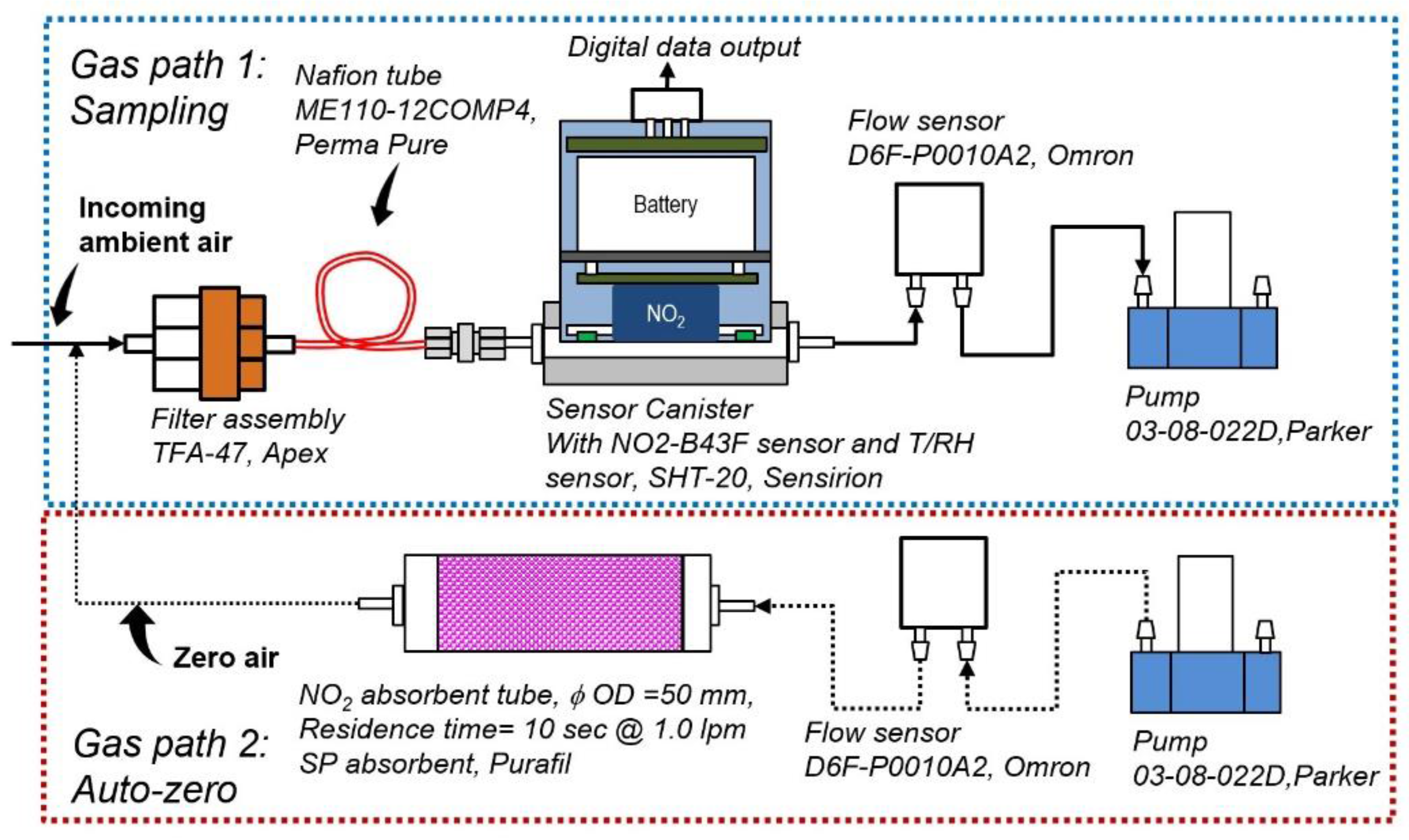
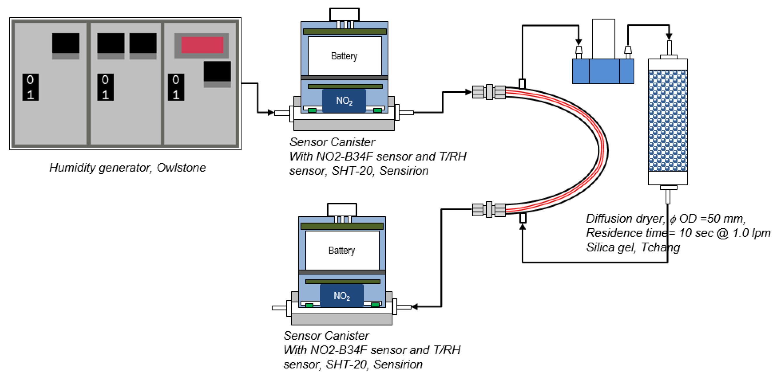
2.1. Test Setup
2.2. NO2 Sensor Calibration
2.3. Performance Test of NO2 Absorbent
2.4. Performance Test of Nafion Tube
2.5. Sensor System Field Test
3. Results and Discussion
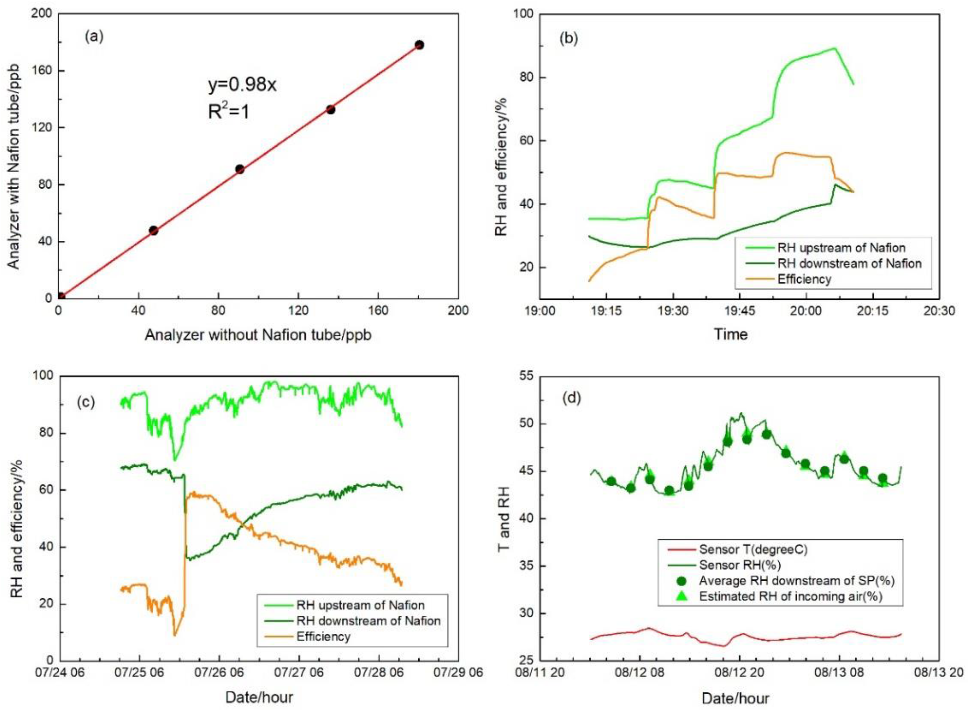
3.1. NO2 Sensor Calibration
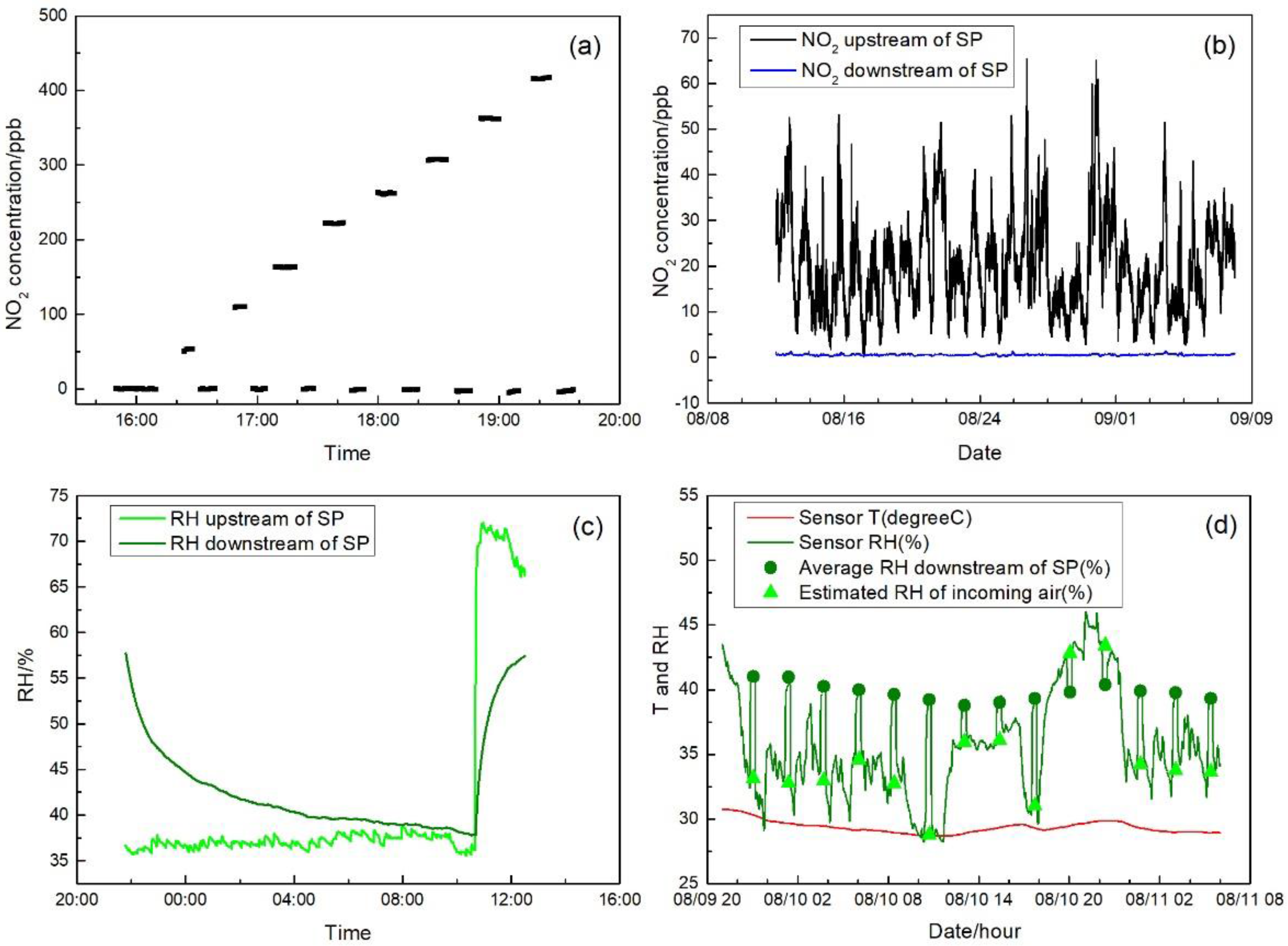
3.2. NO2 Absorbent Performance
3.3. Nafion Tube Performance
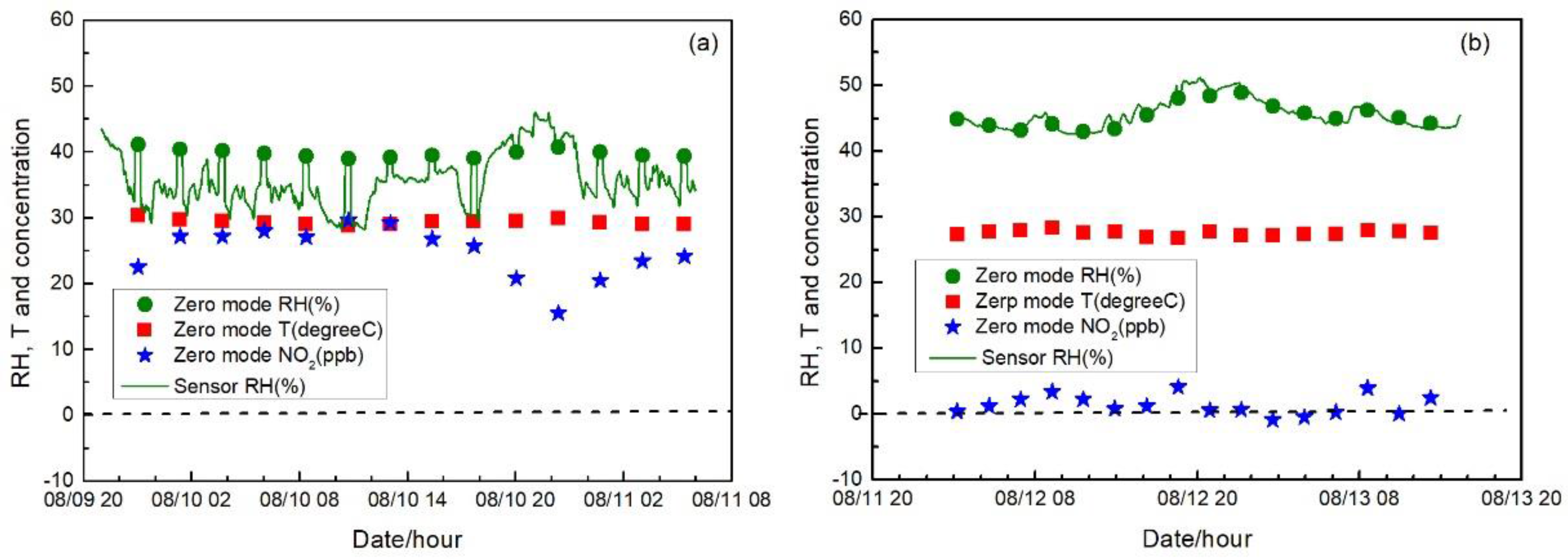
3.4. Impact of Humidity Stabilization on Sensor Output
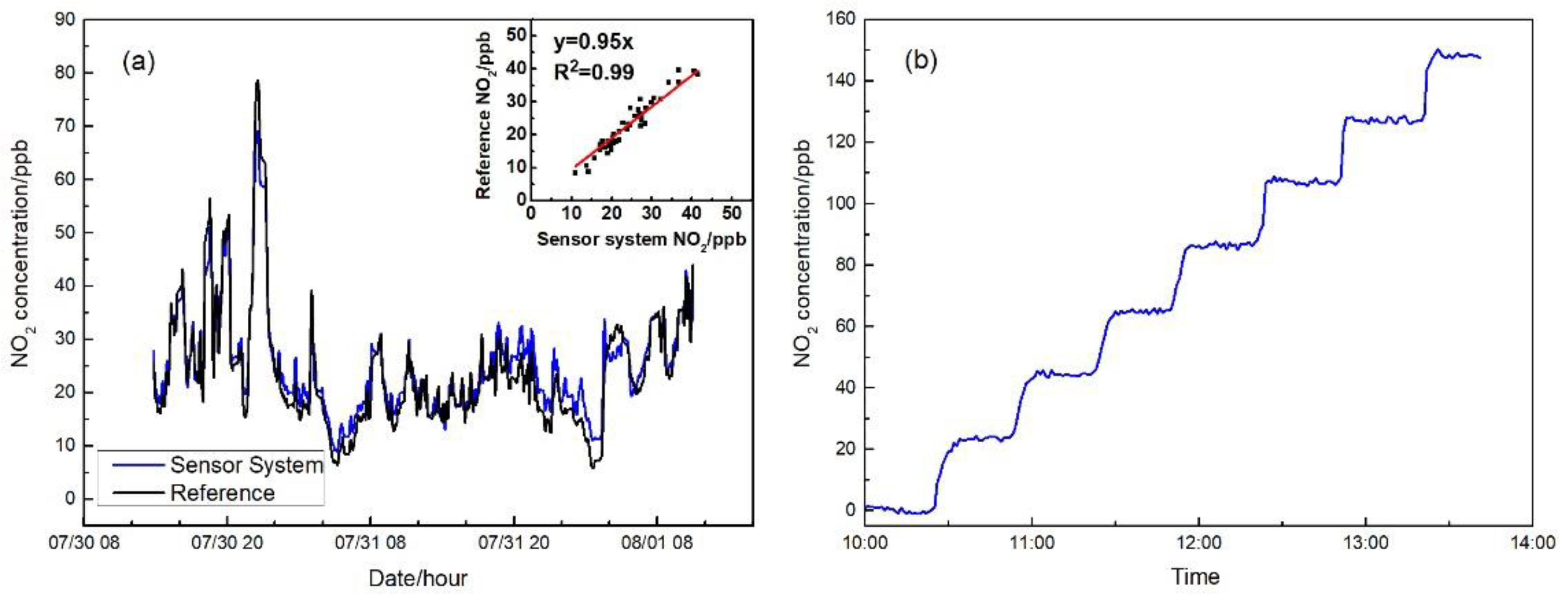
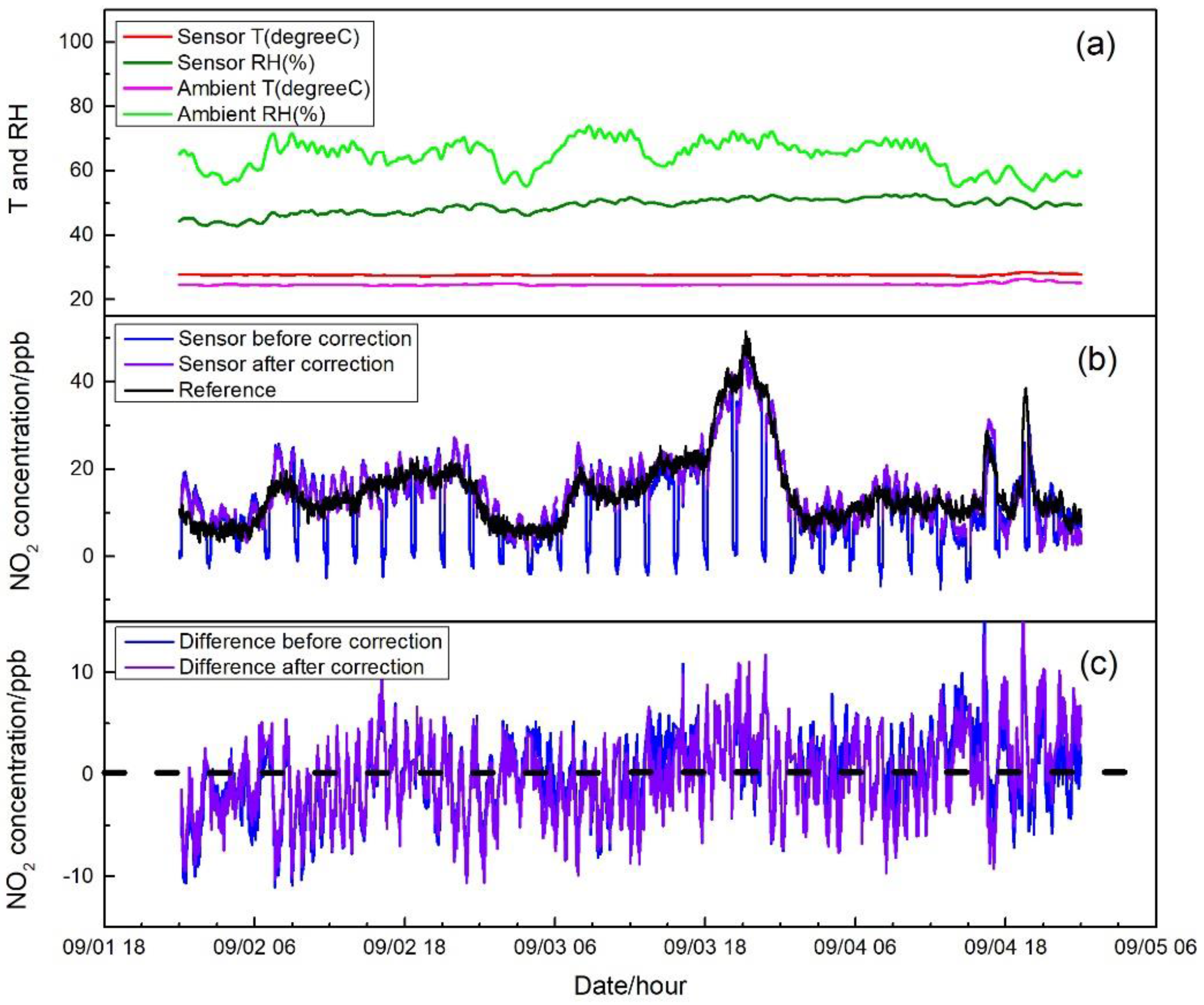
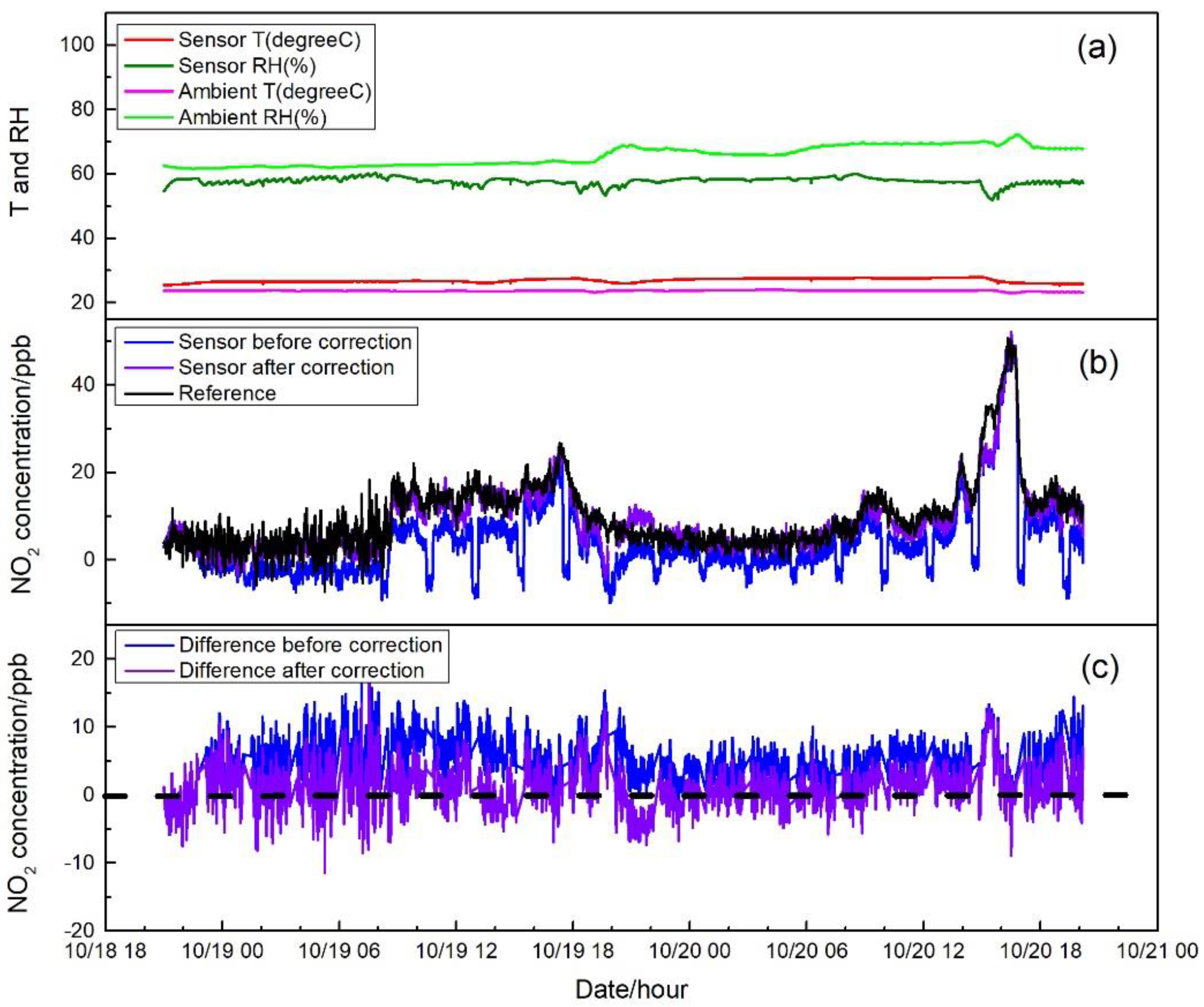
3.5. Sensor System Field Validation
4. Conclusion
Supplementary Materials
Acknowledgments
Author Contributions
Conflicts of Interest
References
- Piedrahita, R.; Xiang, Y.; Masson, N.; Ortega, J.; Collier, A.; Jiang, Y.; Li, K.; Dick, R.P.; Lv, Q.; Hannigan, M.; et al. The next generation of low-cost personal air quality sensors for quantitative exposure monitoring. Atmos. Meas. Tech. 2014, 7, 3325–3336. [Google Scholar] [CrossRef] [Green Version]
- Mead, M.I.; Popoola, O.A.M.; Stewart, G.B.; Landshoff, P.; Calleja, M.; Hayes, M.; Baldovi, J.J.; McLeod, M.W.; Hodgson, T.F.; Dicks, J.; et al. The use of electrochemical sensors for monitoring urban air quality in low-cost, high-density networks. Atmos. Environ. 2013, 70, 186–203. [Google Scholar] [CrossRef]
- Kumar, P.; Morawska, L.; Martani, C.; Biskos, G.; Neophytou, M.; Di Sabatino, S.; Bell, M.; Norford, L.; Britter, R. The rise of low-cost sensing for managing air pollution in cities. Environ. Int. 2015, 75, 199–205. [Google Scholar] [CrossRef] [PubMed] [Green Version]
- Bart, M.; Williams, D.E.; Ainslie, B.; McKendry, I.; Salmond, J.; Grange, S.K.; Alavi-Shoshtari, M.; Steyn, D.; Henshaw, G.S. High density ozone monitoring using gas sensitive semi-conductor sensors in the Lower Fraser Valley, British Columbia. Environ. Sci. Technol. 2014, 48, 3970–3977. [Google Scholar] [CrossRef] [PubMed]
- Brunekreef, B.; Holgate, S.T. Air pollution and health. The Lancet 2002, 360, 1233–1242. [Google Scholar] [CrossRef]
- Kampa, M.; Castanas, E. Human health effects of air pollution. Environ. Pollut. 2008, 151, 362–367. [Google Scholar] [CrossRef] [PubMed]
- Latza, U.; Gerdes, S.; Baur, X. Effects of nitrogen dioxide on human health: Systematic review of experimental and epidemiological studies conducted between 2002 and 2006. Int. J. Hyg. Environ. Health 2009, 212, 271–287. [Google Scholar] [CrossRef] [PubMed]
- Tsujita, W.; Yoshino, A.; Ishida, H.; Moriizumi, T. Gas sensor network for air-pollution monitoring. Sens. Actuators B Chem. 2005, 110, 304–311. [Google Scholar] [CrossRef]
- Zampolli, S.; Elmi, I.; Ahmed, F.; Passini, M.; Cardinali, G.C.; Nicoletti, S.; Dori, L. An electronic nose based on solid state sensor arrays for low-cost indoor air quality monitoring applications. Sens. Actuators B Chem. 2004, 101, 39–46. [Google Scholar] [CrossRef]
- Spinelle, L.; Gerboles, M.; Villani, M.G.; Aleixandre, M.; Bonavitacola, F. Field calibration of a cluster of low-cost available sensors for air quality monitoring. Part A: Ozone and nitrogen dioxide. Sens. Actuators B Chem. 2015, 215, 249–257. [Google Scholar] [CrossRef]
- Postolache, O.A.; Pereira, J.M.D.; Girao, P.M.B.S. Smart sensors network for air quality monitoring applications. IEEE Trans. Instrum. Meas. 2009, 58, 3253–3262. [Google Scholar] [CrossRef]
- Williams, D.E.; Henshaw, G.S.; Bart, M.; Laing, G.; Wagner, J.; Naisbitt, S.; Salmond, J.A. Validation of low-cost ozone measurement instruments suitable for use in an air-quality monitoring network. Meas. Sci. Technol. 2013, 24, 065803. [Google Scholar] [CrossRef]
- Sun, L.; Wong, K.C.; Wei, P.; Ye, S.; Huang, H.; Yang, F.; Westerdahl, D.; Louie, P.K.; Luk, C.W.; Ning, Z. Development and Application of a Next Generation Air Sensor Network for the Hong Kong Marathon 2015 Air Quality Monitoring. Sensors 2016, 16, 211. [Google Scholar] [CrossRef] [PubMed]
- Venterea, R.T.; Groffman, P.M.; Verchot, L.V.; Magill, A.H.; Aber, J.D.; Steudler, P.A. Nitrogem oxide gas emissions from temperate forest soils receiving long-term nitrogen inputs. Glob. Chang. Biol. 2003, 9, 346–357. [Google Scholar] [CrossRef]
- Heimann, I.; Bright, V.B.; McLeod, M.W.; Mead, M.I.; Popoola, O.A.M.; Stewart, G.B.; Jones, R.L. Source attribution of air pollution by spatial scale separation using high spatial density networks of low cost air quality sensors. Atmos. Environ. 2015, 113, 10–19. [Google Scholar] [CrossRef]
- Wei, P.; Ning, Z.; Ye, S.; Sun, L.; Yang, F.H.; Wong, K.C.; Westerdahl, D. Correction algorithm development and error analysis of electrochemical sensors for ambient air quality monitoring. Sens. Actuators B Chem. 2017. submitted. [Google Scholar]
- Chou, J. Hazardous Gas Monitor; McGraw-Hill Book Company: New York, NY, USA, 2000; pp. 162–163. [Google Scholar]
- Warburton, P.R.; Pagano, M.P.; Hoover, R.; Logman, M.; Crytzer, K. Amperometric Gas Sensor Response Times. Anal. Chem. 1998, 70, 998–1006. [Google Scholar] [CrossRef] [PubMed]
- Saffell, J.; Baron, R.; Hossain, M. Amperometric electrochemical gas sensing apparatus and method for measuring oxidising gases. U.S. Patent 20170016847 A1, 19 January 2017. [Google Scholar]


© 2017 by the authors. Licensee MDPI, Basel, Switzerland. This article is an open access article distributed under the terms and conditions of the Creative Commons Attribution (CC BY) license (http://creativecommons.org/licenses/by/4.0/).
Share and Cite
Sun, L.; Westerdahl, D.; Ning, Z. Development and Evaluation of A Novel and Cost-Effective Approach for Low-Cost NO2 Sensor Drift Correction. Sensors 2017, 17, 1916. https://doi.org/10.3390/s17081916
Sun L, Westerdahl D, Ning Z. Development and Evaluation of A Novel and Cost-Effective Approach for Low-Cost NO2 Sensor Drift Correction. Sensors. 2017; 17(8):1916. https://doi.org/10.3390/s17081916
Chicago/Turabian StyleSun, Li, Dane Westerdahl, and Zhi Ning. 2017. "Development and Evaluation of A Novel and Cost-Effective Approach for Low-Cost NO2 Sensor Drift Correction" Sensors 17, no. 8: 1916. https://doi.org/10.3390/s17081916