Article

Morphological Strategies in Ant Communities along Elevational Gradients in Three Mountain Ranges

1
Department of Environment and Genetics, La Trobe University, Bundoora, VIC 3086, Australia
2
Department of Applied Ecology, North Carolina State University, Raleigh, NC 27606, USA
3
Department of Ecology and Evolutionary Biology, University of Michigan, Ann Arbor, MI 48109, USA
4
Research Centre for Ecological Change, Organismal and Evolutionary Biology Research Programme, Faculty of Biological and Environmental Sciences, University of Helsinki, FI-00014 Helsinki, Finland
*
Author to whom correspondence should be addressed.
Diversity 2024, 16(1), 48; https://doi.org/10.3390/d16010048
Submission received: 12 December 2023 / Revised: 3 January 2024 / Accepted: 4 January 2024 / Published: 12 January 2024
(This article belongs to the Special Issue Diversity, Biogeography and Community Ecology of Ants II)

Abstract

:
Species traits often vary in a coordinated manner, making up an ecological strategy comprised of suites of interrelated traits. Environmental gradients, such as those along elevational gradients, provide an ideal venue in which to examine variation in ecological strategies with the environment. We examined variation in the morphological strategies of ants along elevational gradients on thirteen mountains across three mountain ranges in central and south-eastern Australia. We pitfall-trapped ants, counted and identified workers and measured morphological traits. Most species showed a hump-shaped relationship between occurrence and elevation, and several responded to microhabitat variables. Morphological traits varied along two key axes: “gracility”, where high values indicated longer-legged species with dorsally positioned eyes and smooth, bare cuticles; and “size and darkness”, where species with high values were larger and darker. Analysis of assemblage-weighted means revealed that gracility decreased with temperature and increased with precipitation, suggesting links with desiccation tolerance. Size and darkness increased with UV-B, declined with increasing canopy cover and peaked at mid-temperatures. We thus detected strong shifts in dominant morphological strategies along our elevational gradients. However, the multifunctionality and interrelatedness of traits and the covariance of climatic factors may make isolation of the function of individual traits difficult. Further, the predictive power of our models may be limited in the context of novel environments predicted under global change.

1. Introduction

In recent decades, species traits have come to the fore as a potential solution to improving generality in ecology [1]. Recognition of the interrelatedness of traits means that research is increasingly focused on ecological strategies, which comprise suites of traits that vary in a coordinated fashion [2,3]. Local assemblages consist of a subset of species from the regional pool, filtered by their traits [4]. Local assemblages often support a large proportion of global variation in traits, e.g., 74% of variation in CTmax (critical thermal maximum) [5], because local habitats support a large variety of niches. At larger scales, macroecological studies have revealed that further variation in traits can be driven largely by climate [6,7].
In animals, latitudinal gradients in body size, form and colour are long-established examples of how traits vary with the environment at large scales [8,9]. However, the mechanisms driving relationships of these traits with environmental gradients are often unclear, with patterns in different studies often contradictory [10,11]. For example, body size tends to increase in colder environments, but it is unclear whether this is due to thermal inertia, resistance to starvation, desiccation tolerance, or combinations of these mechanisms [12,13]. Ectotherms are often darker in cold environments, but competing hypotheses suggest that this could be due to more rapid absorption of solar radiation (thermal melanism), protection from harmful solar radiation (photo-protection) or increasing desiccation tolerance [14]; in contrast, Gloger’s rule suggests darker colouration is associated with warm and wet climates due to a range of other mechanisms, including camouflage, parasitism resistance and photo-protection [15]. Recent studies suggest that body size and lightness (i.e., the opposite of darkness) are associated and may form a thermoregulatory trade-off in ectotherms, with size-related thermal inertia counter-balanced by lightness-related thermal inertia [16,17,18,19]. This suggests that, in some cases, suites of traits vary in a coordinated fashion and may be better considered as an ecological strategy [2,3].
As anthropogenic climate change accelerates [20], it is increasingly important that we understand the relationship between species’ ecological strategies and climate if we are to predict the consequences for ecosystems. Conditions change rapidly along elevational gradients [21], with climates becoming colder and wetter and solar radiation exposure increasing as elevation increases. Elevational gradients are thus expected to act as a microcosm for the influence of climate change. Climate drives animal species responses directly, through impacts on their morphology, life history, physiology and behaviour [22,23,24,25]. However, it also has indirect effects on species, particularly by altering the structure of their habitats [26,27], which, in turn, drive microclimates, and regulate interactions with other species [28]. Changes in species traits with elevation have been documented across a wide variety of taxa and ecosystems [17,22,25]. Responses are often expressed through changes in the relative abundance of species [17], with many ecological strategies able to coexist in any local assemblage, but the environment determining those that become most abundant. Although plant-based studies commonly consider these changes in terms of ecological strategies, this approach has only rarely been used for animals outside of metabolic scaling and pace of life theories [29,30,31]. Gibb et al. [3] recently suggested that social insects such as ants may be particularly amenable to the ecological strategy approach due, in part, to similarities with plants. For example, both taxa can be considered central place foragers with expendable resource-harvesting units, i.e., leaves and worker ants [3,32].
Ants are diverse and ecologically important in most habitats globally [33,34], comprising a large percentage of animal biomass [35,36]. Their morphological traits have been relatively well-studied and previous studies have detected key morphological changes in response to climate, habitat structure and elevation [13,37]. For example, species living in colder environments are generally larger than those in warmer environments [8,13], those at higher elevations are both larger and darker than those at lower elevations [17], thermophilic and open-habitat ants have longer legs than non-thermophilic and closed-habitat ants [38,39], while correlated cuticle traits such as pilosity and sculpturing are indicative of desiccation tolerance [40,41]. Studies have attempted to deal with this covariation in traits using multivariate approaches to identifying categorical trait-based functional groups, e.g., [42,43]. More recently, we highlighted that ant traits often co-vary, so may be better considered as part of a continuous ecological strategy [3]. This thinking can also be applied to suites of morphological traits: for example, in ants, species with longer limbs generally also have longer antennae and dorsally positioned eyes, making up a ‘gracile’ morphological strategy [3,44].
Here, we examine morphological change along a suite of elevational gradients in three mountain ranges in central to south-eastern Australia. We ask the following questions: (1) What are the key axes of variation in morphological strategies of ants? (2) How does ant assemblage composition vary with elevation and habitat? and (3) How do morphological strategies of local ant assemblages respond to climatic and habitat factors that vary with elevation?

2. Materials and Methods
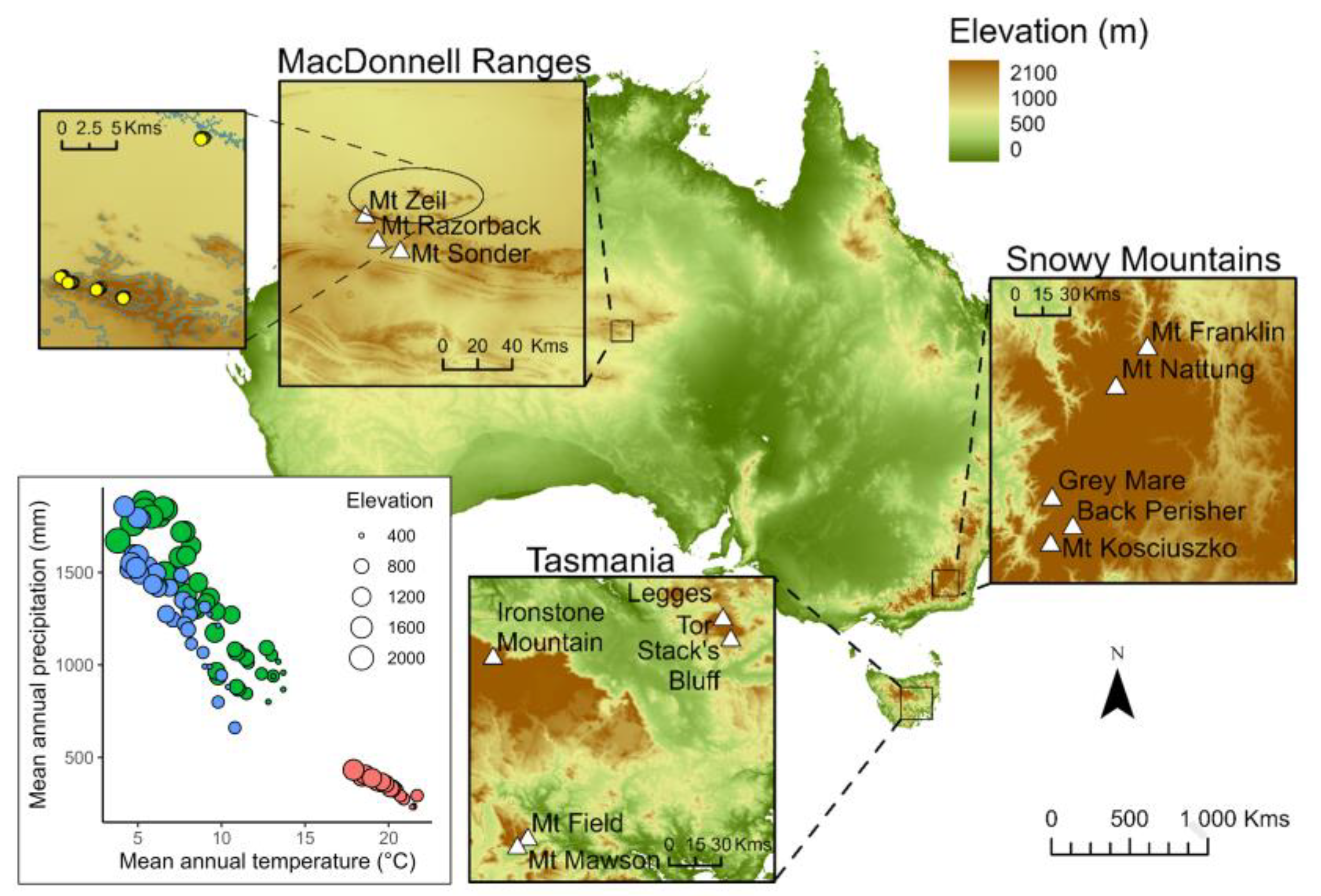
2.1. Study Sites

Field work was conducted along multiple elevation transects (total of 13 mountains) across three of the highest elevation regions in Australia: the MacDonnell Ranges (Mt Giles, 1389 m a.s.l., Mt Sonder 1380 m, and Mt Zeil, 1531 m) in central Australia, the Snowy Mountains in the Great Dividing Range (transects along Mt Back Perisher 2014 m, Mt Franklin 1646 m, Mt Grey Mare 1870 m, Mt Kosciuszko 2228 m and Mt Nattung 1625 m) in south-eastern Australia, and in Tasmania (Legges Tor 1572 m, Stacks Bluff 1527 m, Mt Field 1434 m, Mt Mawson 1318 m and Ironstone Mountain 1444 m) (Figure 1, Table S1). Mean annual temperatures at the study sites range from 17.9 to 21.7 °C for the MacDonnell Ranges, 3.8 to 13.7 °C for the Snowy Mountains, and 4.2 to 10.8 °C for Tasmania. Mean annual precipitation ranges from 231 to 432 mm for the MacDonnell Ranges, 800 to 1878 mm for the Snowy Mountains, and 660 to 1856 mm for Tasmania. UV-B of the highest month ranged from 7281 to 7473 mW.cm−2 for the MacDonnell Ranges, 6406 to 6669 mW.cm−2 for the Snowy Mountains, and 5330 to 5844 mW.cm−2 for Tasmania. Tasmanian sites were sampled in December 2012, the Snowy Mountains in January 2013, and the MacDonnell Ranges in May 2013.

2.2. Sampling Methods

We conducted pitfall trapping along gradients at elevations between 400 m and 2000 m above sea level in 200 m elevational intervals on each of the mountains, where the maximum elevation was determined by the height of the mountain. Ten pitfall traps (8 cm in diameter and 7 cm in depth) were placed in a two by five formation along the mountain side, with traps separated by ten metres. Traps were buried flush with the ground, filled with 100% propylene glycol to 1 cm depth and left out for seven days each.
At each site, we recorded the site aspect and noted coarse woody debris cover (low, medium or high) and dominant vegetation. At each pitfall location, we used a cover estimator chart to make visual estimates of the percentage canopy, summed percentage of the canopy and understorey cover (cover as observed by epigaeic organisms) and the percentage of bare ground (including rock and bare soil), leaf litter, grass, other ground cover plants and moss within a 1 m radius of the pitfall trap location.
In the laboratory, we separated ants from other material and transferred them to vials with 80% ethanol (20% water). We counted ants and identified ants to genus and morphospecies in the laboratory and the identity of reference specimens was determined by Prof. Alan Andersen (Charles Darwin University, Darwin, Australia). We considered both occurrence (number of pitfalls per site in which a species was present) and abundance (total number of workers of each species collected per site).

2.3. Morphological Measurements

We measured a subset of the suite of morphological traits recommended and tabulated in Parr et al. [45], consistent with the Global Ant Database (globalants.org, 01/01/2014) [13] on six specimens for monomorphic species and ten specimens for polymorphic species. The traits measured were head width across eyes (mm), mandible length (mm), hind femur length (mm), inter-ocular width (mm), sculpturing (ordinal measure, 0–3), pilosity (count of hairs crossing the mesosoma profile) and the dominant colour of the mesosoma (see [45] Tables 2 and 3 for details). Eye position was calculated as the residual of (head width—inter-ocular width) with head width.

2.4. Statistical Analysis

Statistical analyses were conducted using R [46]. To describe habitats and reduce the dimensionality of habitat characteristics measured at each pitfall trap, we used principal component analysis (PCA) (prcomp on R) to determine the key axes of variation, standardising all variables. We calculated the site means of habitat variables from the ten pitfall measures for each transect at each elevation for every mountain to use in the analysis. The two principal component axes contributing most to the variation in habitat characteristics among the sites were used in hierarchical modelling of species communities (HMSC).
We used PCA to determine the key axes of morphological variation among species (“ant morphological strategy axes”). Head width was used as a measure of body size and we calculated the residuals of other continuous morphometric measures (femur length, mandible length, eye position) and pilosity (count) with head width to use in the analysis, as these traits are generally highly correlated [45]. The final analysis included head width across the eyes, residual mandible length, residual hind femur length, residual pilosity, residual eye position and lightness of the mesosoma. These traits were reduced to two key morphological strategy axes of “gracility” and “size and darkness” (described in results).
To examine the effects of elevation (made up of the terms “elevation” and “elevation2”, to account for humped relationships with elevation) and habitat variation (principal components PC1 and PC2 from the habitat PCA) on the distributions of ant species and their traits on each mountain range (accounting for the random effect of transect), we used hierarchical modelling of species communities HMSC, Rpackage“hmsc” [47]. HMSC is a joint species distribution model with a hierarchical structure that allows us to model species responses to environmental covariates, and to ask how these depend on species traits and phylogenetic relationships [48,49]. To model the relationship between species’ traits and their environmental responses to each covariate, we included a matrix of the two key morphological strategy axes “gracility” and “size and darkness”.
We accounted for possible phylogenetic correlations in the species’ responses to the environmental variables, in addition to that explained by traits included in the analyses [48], by including an ant phylogeny in the model. Phylogenetic relationships were accounted for by including a species-level phylogeny constructed by Economo et al. [50], which was simplified to genus level by retaining the middle species in each genus (i.e., that occupying the most central of the branches occupied by that genus). We then created polytomies to represent the study species. We excluded rare species (those present at <5 sites) from the HMSC analysis as rare species cannot be modelled reliably [51]. The ant phylogeny was converted into a phylogenetic correlation matrix and used to test for evidence of phylogenetic structure in the residual variance in species environmental responses (after accounting for their traits). The estimated phylogenetic correlation parameter, rho (ρ), takes values from 0 to 1, depending on whether residual variance in environmental responses is independent (0) to fully structured (1) by the phylogenetic relatedness of taxa. Because species assemblages and habitat components differed substantially among mountain ranges, we conducted separate HMSC analyses for each of the three mountain ranges. We assessed MCMC convergence by examining the potential scale reduction factors [52] of the model parameters (i.e., the beta (species–environment relationship) and gamma (trait–environment relationship) parameters of HMSC) [49]. We initially modelled both species occurrence and abundance data, but were unable to obtain satisfactory model convergence for species abundance, perhaps due to its high among-site variability, so we present only the species occurrence results.
We fitted the HMSC models with the “sampleMcmc” function in the “Hmsc” package. We sampled the posterior distribution with four Markov Chain Monte Carlo (MCMC) chains, each of which was run for 37,500 iterations, of which the first 12,500 were removed as burn-in. The chains were thinned by 100 to yield 250 posterior samples per chain. For species–environment models for each mountain range, we extracted the signs of the beta parameters (positive, negative or no response) with at least 95% posterior support. To explore the link between species traits and their environmental niches for each mountain range, we extracted the signs of the gamma parameters (positive, negative or no response) with at least 95% posterior support. We also show relationships with a lower level of statistical support (75% posterior probability) for species–environment and trait–environment models. Finally, we extracted the median value of the rho parameter with its 95% credible interval (i.e., the Bayesian 95% credible interval).
We calculated the assemblage-weighted means (AWM) for the first two ant morphological strategy axes (PC1 and PC2 from the principal component analysis of ant morphology). For assemblage-weighted means, the trait value for each individual in the community is weighted equally, such that numerically dominant species have a greater influence on the AWM than rarer species. AWMs were calculated for each plot without missing values (n = 215):
A W M = i = 1 S p i x i
Here, S is the number of species in the assemblage, pi is the proportional abundance of each species, and xi is the trait value (ant morphological strategy axis PC1 or PC2).
We also used linear mixed effects models lmer from the lme4 package on R [53] to understand the broader assemblage-wide responses of morphological strategy to the climate. Here, we tested the effect of climate (mean annual temperature, mean annual precipitation and mean UVB of the highest month) and habitat (PC1 and PC2 from the principal component analysis of habitat) on the assemblage-weighted means (AWM) of ant morphological strategy axes (PC1 and PC2 from the principal component analysis of ant morphology). Mean annual temperature and mean annual precipitation were taken at 30 arcsec resolution from WorldClim [54], which covers the period 1970–2000. Mean UVB of the highest month was obtained at 15 arcmin resolution from the glUV dataset [55], which covers the years 2004–2013. We also tested key traits for each component (pilosity and eye position for PC1 and lightness and head width for PC2) individually. Mountain peak, nested within mountain range, was included as a random factor. We used the “dredge” function on MuMIn [56] to determine the best model and models within 2 AIC of the best model.

3. Results

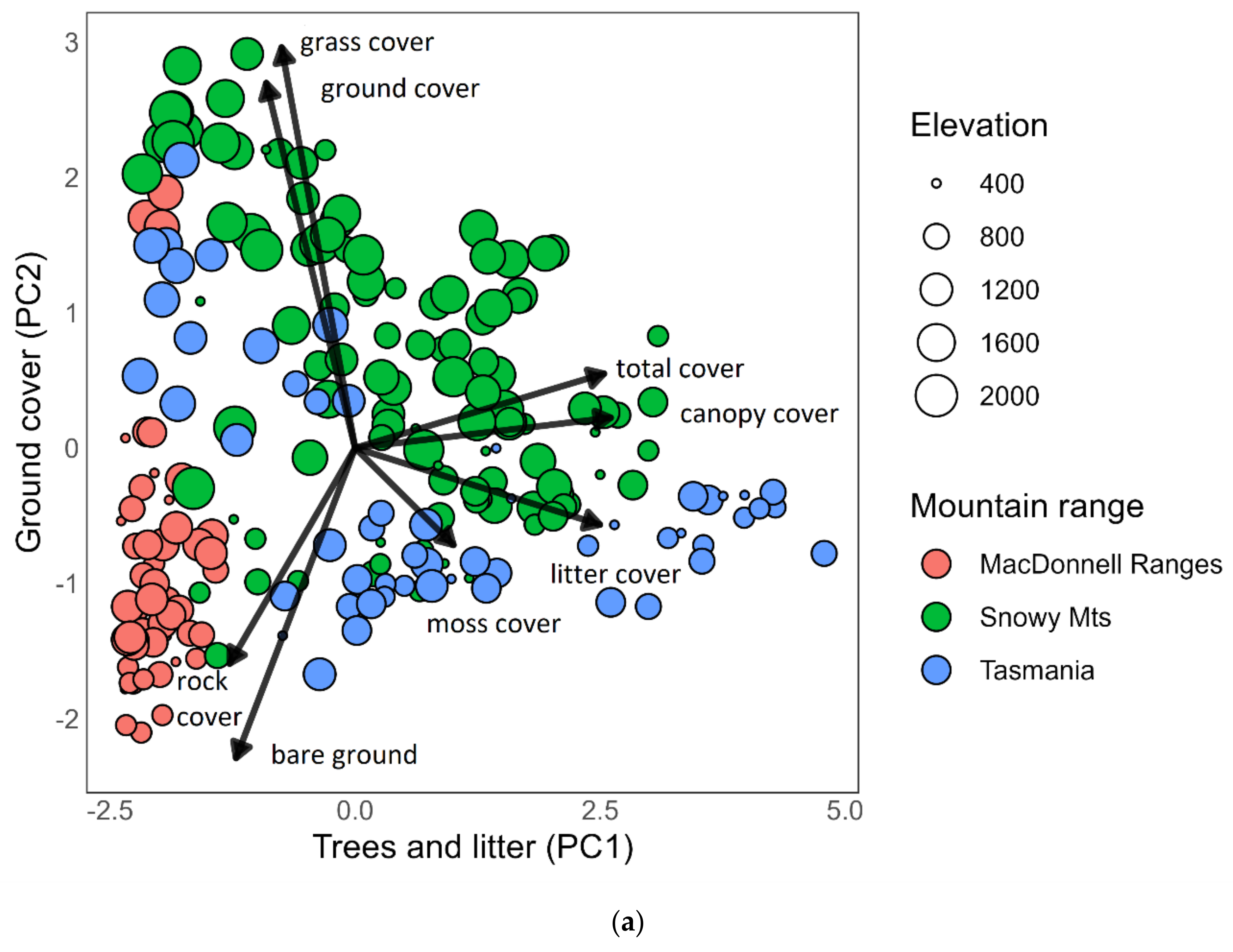
3.1. Microhabitat Composition among Mountain Ranges and Elevations

Principal component analysis of the habitat characteristics data revealed that the first two major axes of variation contributed to 40% and 16% of the variation in habitats, respectively (Table S2). PC1 was positively associated with canopy cover and leaf litter cover (Figure 2a). PC2 was positively associated with rock and bare ground and negatively associated with ground cover and grass (Table S2). The MacDonnell Ranges sites varied minimally along PC1, mostly lacking tree cover and leaf litter. At the MacDonnell Ranges, there were no clear patterns of covariance between elevation and PC2, with sites at most elevations tending toward lower ground cover. An exception to this was a few high elevation sites that had high grass and ground cover (Figure 2a). Both the Tasmanian mountain ranges and the Snowy Mountains exhibited a broader spread along PC1, indicating that canopy and litter cover were more extensive at these sites, particularly in Tasmania. These mountain ranges also included sites with a broad range of ground cover types. High litter cover at sites with abundant canopy cover meant that those sites had little bare ground or ground vegetation (ground cover or grass cover). The highest elevation sites tended to have little canopy cover or leaf litter, but abundant ground vegetation.

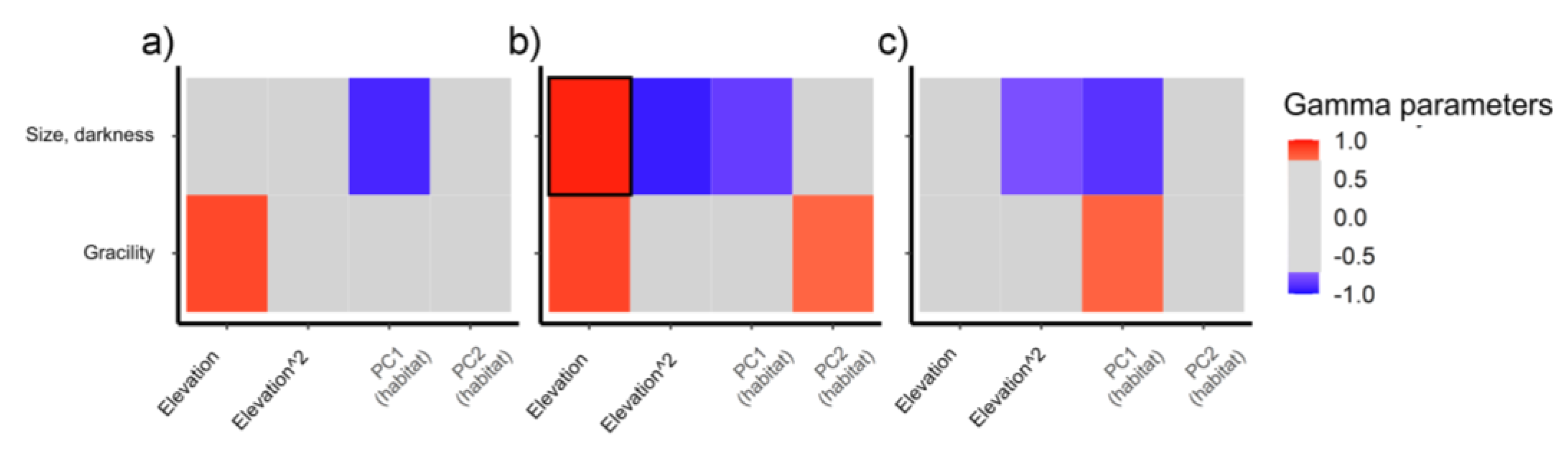
3.2. Effects of Elevation and Microhabitat on Ant Assemblage Composition

Species responses to elevation varied among mountain ranges. In the two cooler mountain ranges (Tasmania and the Snowy Mountains), most species showed humped relationships between abundance and elevation (negative relationship with the polynomial term for elevation), with many species increasing in abundance between low and mid-elevations, but declining at high elevation (Figure 3). In the hot arid mountain range (MacDonnell Ranges), several species declined with increasing elevation (negative relationship with the linear term for elevation) and humped patterns were less common. Declines with elevation were most common in the subfamily Myrmicinae, which includes genera that tend to be small and light-coloured (Figure 2b), such as Meranoplus, Monomorium, Pheidole, Strumigenys and Tetramorium. In Tasmania, many species declined with increasing canopy and litter cover and with increasing ground cover. In the other mountain ranges, patterns were mixed, with similar proportions of positive and negative responses to habitat measures. Across mountain ranges, several taxa, including Rhytidoponera and Iridomyrmex, responded negatively to increasing canopy and litter cover, but different species within the same genus often showed different patterns. In response to increasing ground cover, we observed declines in taxa such as the thermophilic Melophorus and some dolichoderines.

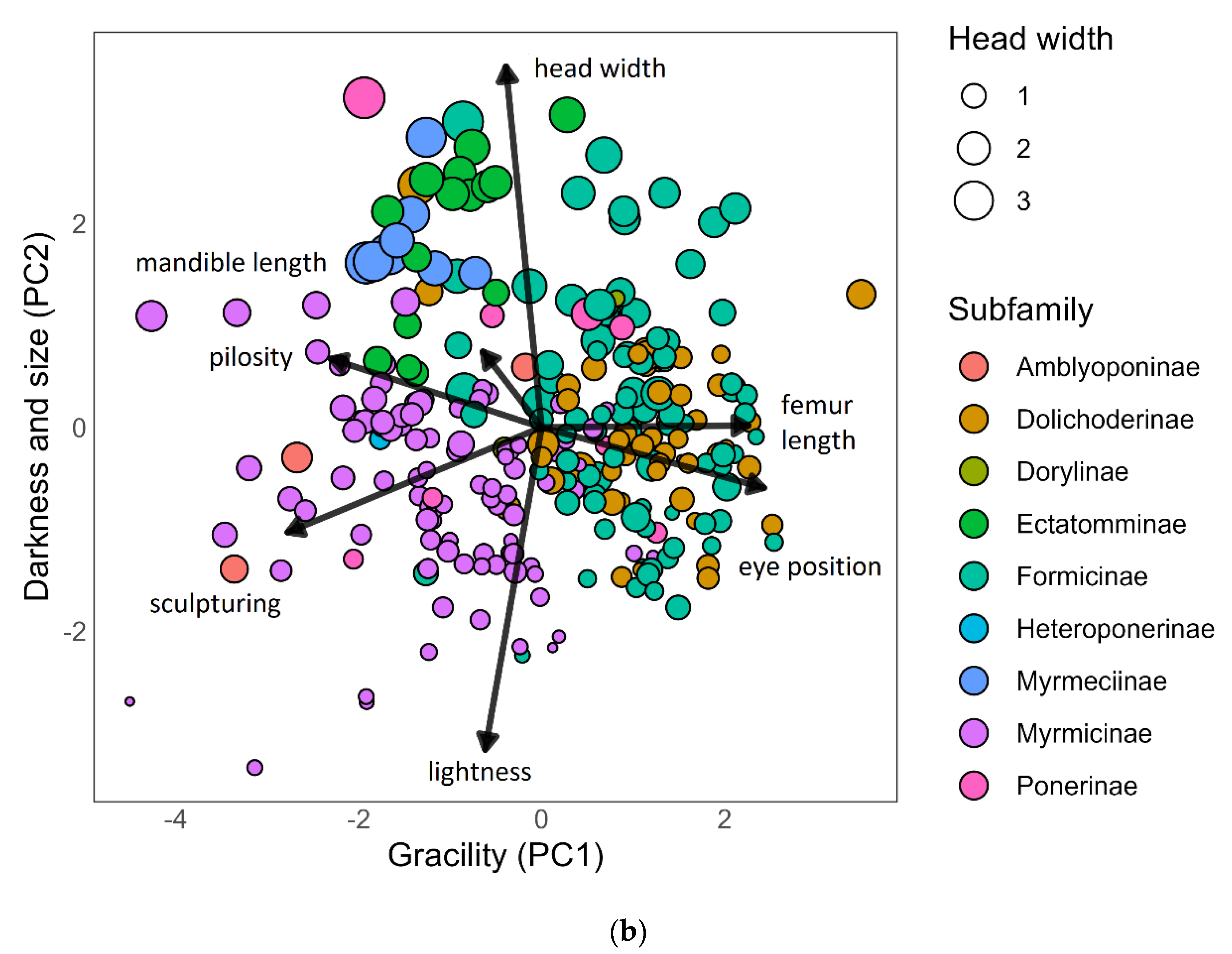
3.3. Morphological Trait Variation among Subfamilies

Principal component analysis of ant morphological traits revealed that PC1 and PC2 contributed to 28.7% and 19.0% of variation in the data, respectively (Figure 2b). PC1 was positively associated with femur length and eye position and negatively associated with cuticle sculpturing and pilosity. PC2 was positively associated with mesosoma darkness and head width. Subfamilies clustered within this space, with formicines and dolichoderines tending to have eyes more dorsally positioned and to have a more gracile body form, with longer legs (femur length). Myrmecia (the sole genus in Myrmeciinae) were characterised by large body size and long mandibles. Ectatommines also tended to be large and dark. Myrmicines were characterised by small size, robust body form, more laterally positioned eyes, lighter colour and greater pilosity.
HMSC analyses of the trait–environment relationships on each mountain (again using elevation, the polynomial degree 2 term for elevation, and the two habitat principal components) revealed several relationships between species’ traits and their predicted environmental niches (Figure 4). Size and darkness had a positive relationship with species’ elevational distributions in the Snowy Mountains at >0.95% posterior probability, with less evidence of a peak at higher elevations. Size and darkness also decreased with PC1 (trees and litter) at all mountain ranges at >0.75 posterior probability. Gracility increased with elevation in the MacDonnell Ranges and Snowy Mountains with >0.75% posterior probability. The median estimated phylogenetic independence parameter indicated that the phylogenetic signal was very weak in the MacDonnell Ranges (ρ = 0.06, posterior probability = 0.27%) and Tasmania (ρ = 0.08, posterior probability = 0.29%) and somewhat stronger, but still with low support in the Snowy Mountains (ρ = 0.36, posterior probability = 0.81%). This suggests a relatively small contribution of phylogenetic relatedness to the outcome of the analysis.

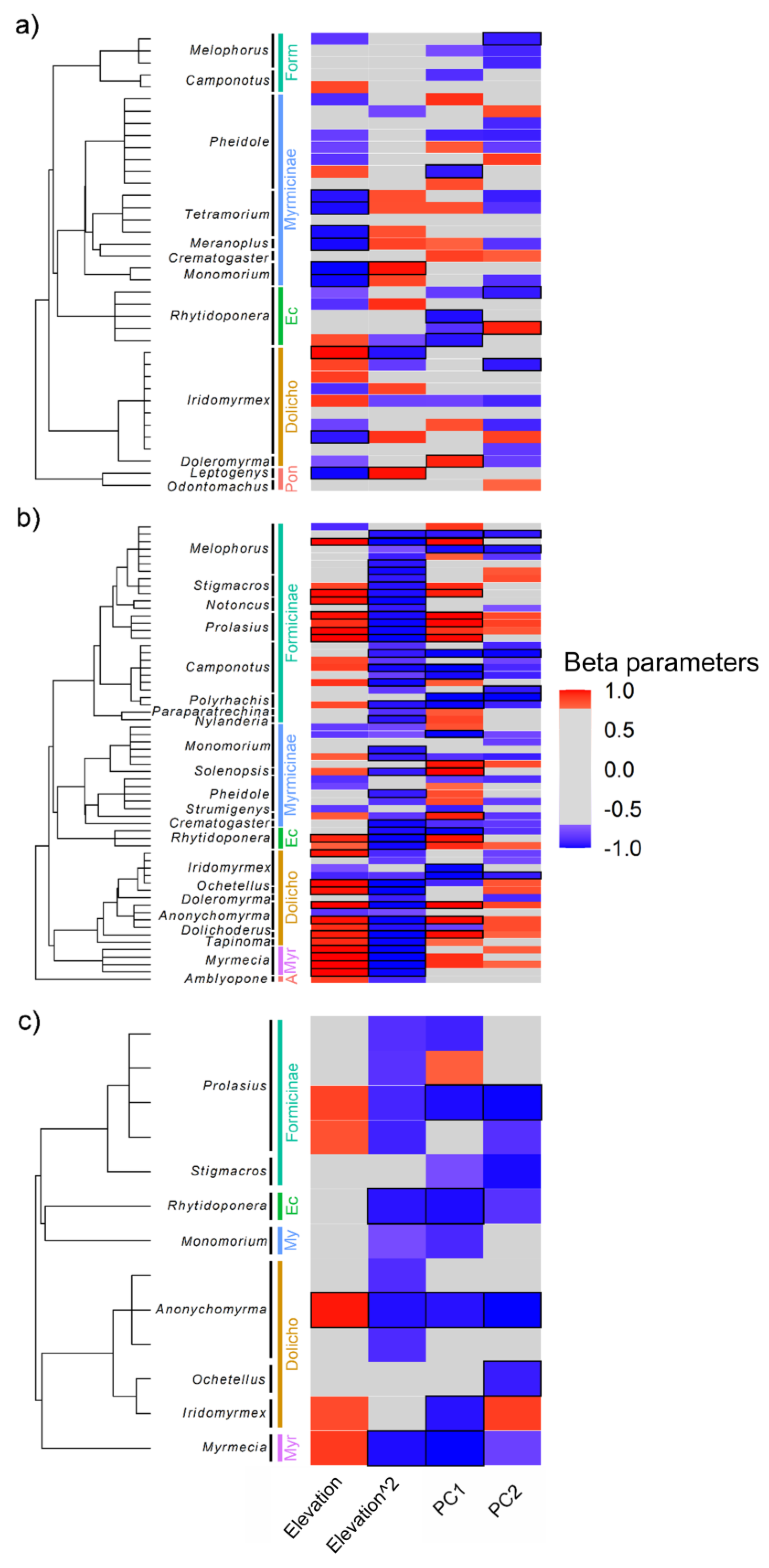
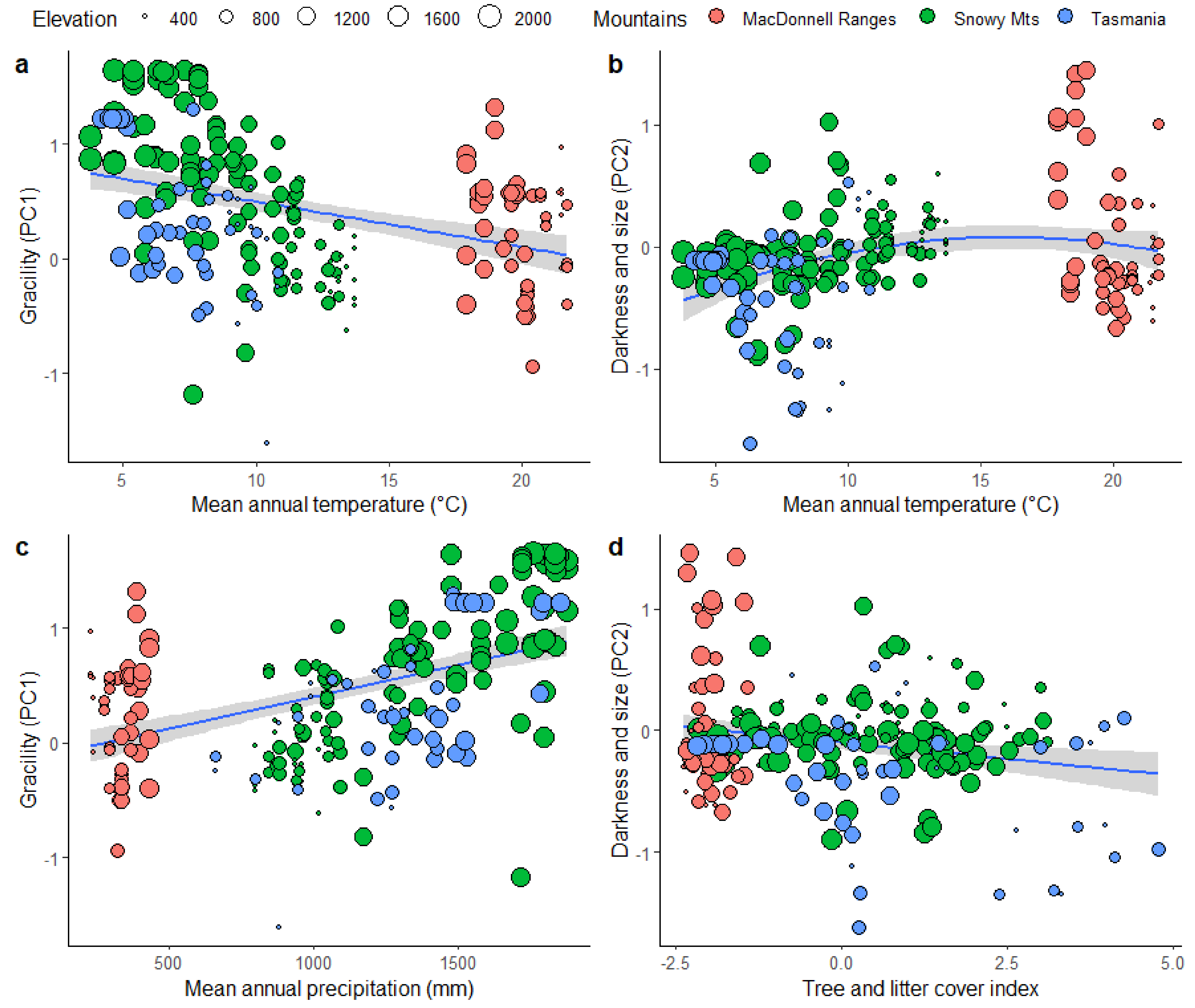
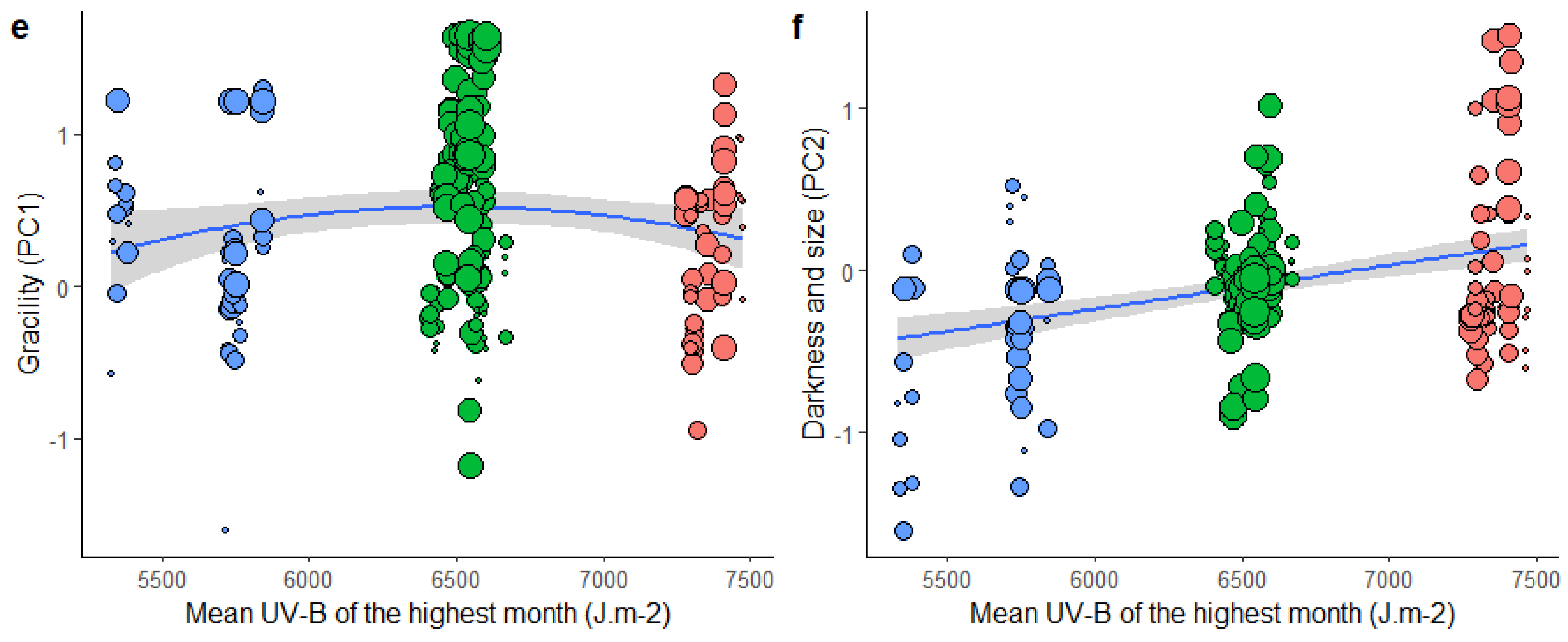
3.4. Effect of Climate and Microhabitat on Morphological Strategies across Mountain Ranges

Model selection on linear mixed models revealed that, across the suite of sites, climatic variables were generally more important than habitat variables in determining the assemblage-weighted mean of morphological strategy axes. Compared with the HMSC traits models, these models did not correct for phylogenetic similarity, but weighted species based on their numerical dominance, therefore indicating the ecological success of morphological strategies. Models within 2 AIC of the best models for both PC1 “gracility” and PC2 “size and darkness” all included mean annual temperature and UV-B (Table 1 and Table 2, Figure 5a,c,e). The fit of the best model for gracility (R2m = 0.47 and R2c = 0.50, including UVB, MAT and MAP) was better than the fits of the best models of key component pilosity (R2m = 0.27 and R2c = 0.32, including UVB, MAP and both habitat components) and eye position (R2m = 0.36 and R2c = 0.39, including MAT and canopy and litter cover). The fit of the best model for size and darkness (R2m = 0.24 and R2c = 0.33, including MAT, UV-B and canopy and litter cover) was less than the fit to lightness alone (R2m = 0.37 and R2c = 0.49, including only MAT and UV-B), but not size alone (R2m = 0.24 and R2c = 0.33, including MAT and canopy and litter cover). Gracility (numerical dominance by gracile species) declined with increasing mean annual temperature and displayed a weak U-shaped relationship with UV-B. Gracility also increased with mean annual precipitation. Models within 2 AIC of the best models for size and darkness included UV-B, habitat PC1, mean annual temperature and sometimes mean annual precipitation. Size and darkness (numerical dominance by large, dark species) peaked at intermediate mean annual temperatures, declined with increasing canopy and litter cover (habitat PC1) and increased with UV-B (Table 1 and Table 2, Figure 5b,d,f).

4. Discussion

We examined associations between ant assemblage composition, ant morphological strategies and the environment along elevational gradients on thirteen mountains across three mountain ranges, two in temperate south-eastern Australia and the third in arid central Australia. These gradients captured environmental variation in climate, openness and litter cover as well as extreme trait variation (Figure 2a). Individual species responded idiosyncratically to elevation and habitat structure, but we observed a general trend toward humped occurrence patterns at the temperate sites, where climatic conditions varied more across the gradient. Ant morphologies occupied two key axes of “gracility” and “size and darkness”, suggesting that suites of traits are interrelated, presenting important morphological strategies. When we accounted for species abundances by considering assemblage-weighted mean responses of ant morphological strategies, we detected clear responses to the environment. Although assemblages in all mountain ranges supported a broad range of morphological strategies, our study thus suggests that dominant morphological strategies are regulated by climate.

4.1. Assemblage Composition along Elevational Gradients

Species assemblages varied in their response to elevation among mountain ranges. In the temperate mountain ranges, many species increased in abundance with elevation to a point, then decreased (showing a humped relationship). A decline with increasing elevation was particularly common among the myrmicines, which are smaller and lighter in colour than most other subfamilies present and were most diverse in leaf litter environments. Although several species declined with elevation in the MacDonnell Ranges, overall patterns were more idiosyncratic, reflecting lower variation in climatic variables among sites: mean annual temperatures varied less than 4 °C among sites in the MacDonnell Ranges, but more than 10 °C for the Snowy Mountains and 6 °C in Tasmania. Similarly, mean annual precipitation in the MacDonnell Ranges varied less than 200 mm among sites, while that in the Snowy Mountains varied by 1000 mm and Tasmania by 1200 mm. This is also reflected in the low variation in microhabitats in the MacDonnell Ranges, compared with the south-eastern mountain ranges.
At all sites, greater ground cover was associated with a lower occurrence of several species (at >95% probability), particularly species within the thermophilic genus Melophorus. Patterns were more idiosyncratic when a broader band of certainty was considered (>75%). Greater tree and litter cover was associated with a reduced occurrence of several ant species in Tasmania, consistent with the finding that cool forest environments are less favourable than grasslands and shrublands for ants [36]. More broadly, Iridomyrmex and Rhytidoponera declined in occurrence with increasing canopy cover, consistent with known preferences of Iridomyrmex and large species of Rhytidoponera for open habitats [28,57]. Globally, ant species richness increases with temperature and precipitation [58]. Although mean annual temperatures may be higher at low elevations, high canopy cover may reduce access to solar radiation relative to high elevation sites, which lack canopy cover. Ants do not need to be active year-round, so the occurrence of warmer conditions during summer days may favour ant species able to optimise their foraging activity during those times.

4.2. Changes in Morphological Strategy in Relation to the Environment

4.2.1. Gracility

Changes in species dominance across mountain ranges and elevations were linked with the morphological strategy axes of “gracility” and “size and darkness”. Our “gracility” axis aligns well with a global-scale description of the major axes of morphological variation in ants [3]. Increasing “gracility” indicated species with relatively longer legs, more dorsally positioned eyes and barer (less pilose), less sculptured cuticles (Figure 2b). Formicines and dolichoderines tended to be more gracile, while myrmicines, amblyoponines and ponerines were less gracile. Dominance by gracile species declined with increasing temperature and decreasing rainfall, suggesting that robust, hairy morphologies are favoured in hot and arid conditions, probably because they protect against desiccation [41]. Fits for the composite “gracility” variable were better than those for its key components. Extreme long-leggedness is usually associated with thermophily as it allows ants to raise the body into cooler air layers and increase running speeds, resulting in reduced foraging times and therefore less heat exposure [38]. In contrast, gracility tended to increase with increasing elevation (Figure 4), and was low in the (hotter) MacDonnell Ranges, and at lower elevation (hotter, drier) sites in the Snowy Mountains and Tasmania (Figure 5a,c). However, long-limbed species are also likely to have a larger surface area to volume ratio, increasing rates of water loss [59]. In ants, high pilosity and sculpturing are associated with reduced water loss rates and increased temperature tolerance [41], suggesting another mechanism through which low “gracility” increases desiccation resistance. Even sparsely distributed hairs increase boundary layer resistance to water loss in insects, and hydrophobic hairs situated over spiracles may further reduce water loss [60,61,62,63]. The suite of covarying traits that comprises “gracility” may therefore indicate a spectrum of desiccation tolerance. Species that are desiccation-tolerant may trade-off benefits accrued from high gracility, such as forager speed [38], to increase foraging times in more arid environments.
Analysis of the gracility–UVB relationship suggests that gracility may peak at mid UVB. However, this weak response may be a result of the dominance of relatively gracile Iridomyrmex in the Snowy Mountains. Iridomyrmex are named for their iridescent cuticle, with the iridescence arising from cuticle nanostructures [64]. Iridescent hairs increase the reflectivity of Cataglyphis bombycina ants in the visible and near-infra-red and emissivity in the mid-infra-red ranges, enhancing their survival in the hot arid climate of the Saharan desert [65,66]. Structural iridescence in Iridomyrmex cuticles might have similar effects in the high UV environments of central Australia, although the function of cuticular iridescence is unclear: experiments with tiger beetles (Cicindela) were unable to show that cuticular iridescence influences heat gain from solar radiation [67].

4.2.2. Size and Darkness

Along the second morphological strategy axis, size and darkness increased together, with myrmeciines and ectatommines tending to be larger and darker, while myrmicines, dolichoderines and many formicines were smaller and lighter in colour. Darkness and body size are thought to be linked due to interrelated thermal benefits, whereby size-related thermal inertia is counter-balanced by lightness-related thermal inertia [16,18]. However, UV-B is hypothesised to increase cuticle darkness without affecting body size, suggesting the potential for the decoupling of these traits where UV-B and temperature are positively correlated, e.g., [14], this study. Dominance by larger and darker ant species was associated with several environmental factors in the assemblage weighted models, including mean annual temperature, tree and litter cover and UV-B (Figure 5). Consistent with this, large, dark species occurred more at high elevations (in the Snowy Mountains) and less in sites with high tree and litter cover in the HMSC (Figure 4). Mean annual precipitation appeared in the next-best model for size and darkness. The best models for assemblage darkness achieved a better fit than the composite “size and darkness” variable, although those for assemblage size (head width) did not. The best models for assemblage darkness included MAT and UV-B, but not precipitation, suggesting that Gloger’s rule (ants are darker in warmer, wetter environments) [9] was not supported. Melanin, the pigment that makes ant cuticles appear dark, absorbs UV wavelengths such that cuticles containing large melanin concentrations may protect against UV-B wavelength light penetration [17,68,69]. Consistent with the photo-protection hypothesis [14], dominance by larger and darker ant species was strongly associated with increasing UV-B, despite large variation in this axis within mountain ranges. This continent-scale result is consistent with Law et al.’s [14] local-scale study, which showed that ants occupying higher strata in a tropical rainforest were darker. Other studies of ants at global scales have shown weaker relationships between lightness and UV-B [17,70], suggesting there is greater evidence for thermal melanism.
Ectotherms are commonly reported to be larger and darker in cooler environments [13,18,71]. While temperature and “size and darkness” were negatively correlated in the MacDonnell Ranges, increasing temperature was associated with increasing size and darkness for the Snowy Mountains and Tasmanian mountain ranges, resulting in a humped relationship between temperature and the size/darkness morphological axis. The decline in ant size/darkness with increasing temperature in the MacDonnell Ranges is consistent with the thermal melanism hypothesis [71,72] because darker species heat up faster, while larger body size increases thermal resistance [18,59]. However, the increase in size and darkness with increasing temperature in the south-eastern sites contradicts the thermal melanism hypothesis. It also contrasts with Bishop et al.’s [17] finding that assemblage darkness in ants declines with increasing temperature at low UV-B, but not at the most extreme UV-B. The anomaly in the two south-eastern mountain ranges might be associated with their high tree lines: 1800–2000 m in the Snowy Mountains and about 1200 m on mountain peaks in Tasmania [73,74]; and greater ground cover at high elevation sites. Both factors would increase shading and insulation at ground level and protect ants from temperature extremes. While ground cover (habitat PC2) did not appear in the best models, greater tree and litter cover (habitat PC1) was associated with decreased darkness and size. Microhabitats filter the larger-scale climates experienced by species and are therefore a critical consideration in understanding trait–environment links at a scale relevant to species [75,76]. Increasing tree and litter cover likely protects species from harmful UVB and reduces their opportunity to use dark colours to rapidly absorb heat. Litter also creates complex habitats that can be difficult for larger species to traverse [37,77].

5. Conclusions

This study builds the case for the contribution of coordinated variation in traits among ants to ecological strategies. We have identified broad morphological strategies of ants in response to climatic and habitat variables that change in a coordinated fashion along elevational gradients. A variety of functions have been attributed to the traits we have examined here, many of which have been experimentally tested and verified, e.g., pilosity and sculpturing are associated with desiccation tolerance [41]. The multifunctionality of traits suggests that trait covariance may differ among systems if there is no physiological trade-off despite correlations among traits. For example, although size-related thermal inertia is counter-balanced by lightness-related thermal inertia, lightness is also predicted to respond to UV-B, independent of body size. Elevational gradients are unique in the covariance of several climatic variables, e.g., temperature and UV-B are negatively correlated along elevational gradients, but positively correlated along latitudinal gradients, so it is unclear whether the covariance of the suites of traits examined in this study is universal (e.g., through trade-offs). However, this is important information if we are to predict species responses to future novel climates, where associations among climate variables may differ from those found in contemporary environments. We argue that our focus on the coordinated variation of traits as ecological strategies, measured as continuous variables, allows for a predictive science that can better equip us for global change than the placement of taxa into categories, e.g., functional groups [43,78].

Supplementary Materials

The following supporting information can be downloaded at: https://www.mdpi.com/article/10.3390/d16010048/s1, Table S1: Locations and conditions of sampling sites. Abbreviations are as follows: MAT = mean annual temperature, MAP = mean annual precipitation, and UVB = mean UVB of the highest month. Table S2: Eigenvalues and % variance explained by principal components and contribution of habitat characteristics and morphological traits to the primary and secondary principal components from PCA.

Author Contributions

Conceptualization: H.G., N.J.S. and R.R.D.; Methodology: H.G., I.O. and M.P.; Data Analysis: M.M.J., P.C. and H.G.; Writing—Original Draft Preparation: H.G.; Writing—Review and Editing: all authors. All authors have read and agreed to the published version of the manuscript.

Funding

We thank the Australian Research Council for funding this project (DP120100781).

Institutional Review Board Statement

The study was approved by the Ethics Committee of La Trobe University (AEC11-46 01.09.2011).

Data Availability Statement

Data will be deposited in the Global Ant Database (globalants.org).

Acknowledgments

We acknowledge the traditional owners of the lands on which this research was performed: the Arrernte, Ngarigo, Walgal, Nuenonne, Pyemmairrener, Weebonenetiner and Lairmairrener peoples. We thank Alan Andersen for his assistance with ant identification. We are grateful to the field volunteers who assisted with data collection.

Conflicts of Interest

The authors declare no conflicts of interest.

References

  1. McGill, B.J.; Enquist, B.J.; Weiher, E.; Westoby, M. Rebuilding community ecology from functional traits. Trends Ecol. Evol. 2006, 21, 178–185. [Google Scholar] [CrossRef] [PubMed]
  2. Westoby, M.; Falster, D.S.; Moles, A.T.; Vesk, P.A.; Wright, I.J. Plant ecological strategies: Some leading dimensions of variation between species. Annu. Rev. Ecol. Syst. 2002, 33, 125–159. [Google Scholar] [CrossRef]
  3. Gibb, H.; Bishop, T.R.; Leahy, L.; Parr, C.L.; Lessard, J.P.; Sanders, N.J.; Shik, J.Z.; Ibarra-Isassi, J.; Narendra, A.; Dunn, R.R. Ecological strategies of (pl) ants: Towards a world-wide worker economic spectrum for ants. Funct. Ecol. 2023, 37, 13–25. [Google Scholar] [CrossRef] [PubMed]
  4. Kraft, N.J.; Adler, P.B.; Godoy, O.; James, E.C.; Fuller, S.; Levine, J.M. Community assembly, coexistence and the environmental filtering metaphor. Funct. Ecol. 2015, 29, 592–599. [Google Scholar] [CrossRef]
  5. Kaspari, M.; Clay, N.A.; Lucas, J.; Yanoviak, S.P.; Kay, A. Thermal adaptation generates a diversity of thermal limits in a rainforest ant community. Glob. Change Biol. 2015, 21, 1092–1102. [Google Scholar] [CrossRef]
  6. Brown, J.H. Macroecology; University of Chicago Press: Chicago, IL, USA, 1995. [Google Scholar]
  7. Chown, S.L.; Gaston, K.J. Body size variation in insects: A macroecological perspective. Biol. Rev. 2010, 85, 139–169. [Google Scholar] [CrossRef]
  8. Bergmann, C. Uber die verhaltnisse der warmeokonomie der thiere zu ihrer grosse. Gott. Stud. 1847, 1, 595–708. [Google Scholar]
  9. Rensch, B. Some problems of geographical variation and species-formation. Proc. Linn. Soc. Lond. 1936, 150, 275–285. [Google Scholar] [CrossRef]
  10. Meiri, S.; Thomas, G.H. The geography of body size–challenges of the interspecific approach. Glob. Ecol. Biogeogr. 2007, 16, 689–693. [Google Scholar] [CrossRef]
  11. Watt, C.; Mitchell, S.; Salewski, V. Bergmann’s rule; a concept cluster? Oikos 2010, 119, 89–100. [Google Scholar] [CrossRef]
  12. Huston, M.A.; Wolverton, S. Regulation of animal size by eNPP, Bergmann’s rule and related phenomena. Ecol. Monogr. 2011, 81, 349–405. [Google Scholar] [CrossRef]
  13. Gibb, H.; Sanders, N.J.; Dunn, R.R.; Arnan, X.; Vasconcelos, H.L.; Donoso, D.A.; Andersen, A.N.; Silva, R.R.; Bishop, T.R.; Gomez, C.; et al. Habitat disturbance selects against both small and large species across varying climates. Ecography 2018, 41, 1184–1193. [Google Scholar] [CrossRef]
  14. Law, S.J.; Bishop, T.R.; Eggleton, P.; Griffiths, H.; Ashton, L.; Parr, C. Darker ants dominate the canopy: Testing macroecological hypotheses for patterns in colour along a microclimatic gradient. J. Anim. Ecol. 2020, 89, 347–359. [Google Scholar] [CrossRef]
  15. Delhey, K. A review of Gloger’s rule, an ecogeographical rule of colour: Definitions, interpretations and evidence. Biol. Rev. 2019, 94, 1294–1316. [Google Scholar] [CrossRef] [PubMed]
  16. Gates, D.M. Biophysical Ecology; Springer: Berlin/Heidelberg, Germany, 1980. [Google Scholar]
  17. Bishop, T.R.; Robertson, M.P.; Gibb, H.; Van Rensburg, B.J.; Braschler, B.; Chown, S.L.; Foord, S.H.; Munyai, T.C.; Okey, I.; Tshivhandekano, P.G. Ant assemblages have darker and larger members in cold environments. Glob. Ecol. Biogeogr. 2016, 25, 1489–1499. [Google Scholar] [CrossRef]
  18. Schweiger, A.H.; Beierkuhnlein, C. Size dependency in colour patterns of Western Palearctic carabids. Ecography 2016, 39, 846–857. [Google Scholar] [CrossRef]
  19. Moreno Azócar, D.L.; Perotti, M.G.; Bonino, M.F.; Schulte, J.; Abdala, C.S.; Cruz, F.B. Variation in body size and degree of melanism within a lizards clade: Is it driven by latitudinal and climatic gradients? J. Zool. 2015, 295, 243–253. [Google Scholar] [CrossRef]
  20. Elsen, P.R.; Saxon, E.C.; Simmons, B.A.; Ward, M.; Williams, B.A.; Grantham, H.S.; Kark, S.; Levin, N.; Perez-Hammerle, K.V.; Reside, A.E. Accelerated shifts in terrestrial life zones under rapid climate change. Glob. Change Biol. 2022, 28, 918–935. [Google Scholar] [CrossRef]
  21. Graham, C.H.; Carnaval, A.C.; Cadena, C.D.; Zamudio, K.R.; Roberts, T.E.; Parra, J.L.; McCain, C.M.; Bowie, R.C.; Moritz, C.; Baines, S.B. The origin and maintenance of montane diversity: Integrating evolutionary and ecological processes. Ecography 2014, 37, 711–719. [Google Scholar] [CrossRef]
  22. Chown, S.L.; Gaston, K.J. Exploring links between physiology and ecology at macro-scales: The role of respiratory metabolism in insects. Biol. Rev. Camb. Philos. Soc. 1999, 74, 87–120. [Google Scholar] [CrossRef]
  23. Shah, A.A.; Gill, B.A.; Encalada, A.C.; Flecker, A.S.; Funk, W.C.; Guayasamin, J.M.; Kondratieff, B.C.; Poff, N.L.; Thomas, S.A.; Zamudio, K.R. Climate variability predicts thermal limits of aquatic insects across elevation and latitude. Funct. Ecol. 2017, 31, 2118–2127. [Google Scholar] [CrossRef]
  24. DeMarche, M.L.; Doak, D.F.; Morris, W.F. Incorporating local adaptation into forecasts of species’ distribution and abundance under climate change. Glob. Change Biol. 2019, 25, 775–793. [Google Scholar] [CrossRef] [PubMed]
  25. Midolo, G.; De Frenne, P.; Hölzel, N.; Wellstein, C. Global patterns of intraspecific leaf trait responses to elevation. Glob. Change Biol. 2019, 25, 2485–2498. [Google Scholar] [CrossRef] [PubMed]
  26. Jiménez-Valverde, A.; Lobo, J.M. Determinants of local spider (Araneidae and Thomisidae) species richness on a regional scale: Climate and altitude vs. habitat structure. Ecol. Entomol. 2007, 32, 113–122. [Google Scholar] [CrossRef]
  27. Neel, L.K.; Logan, M.L.; Nicholson, D.J.; Miller, C.; Chung, A.K.; Maayan, I.; Degon, Z.; DuBois, M.; Curlis, J.D.; Taylor, Q. Habitat structure mediates vulnerability to climate change through its effects on thermoregulatory behavior. Biotropica 2021, 53, 1121–1133. [Google Scholar] [CrossRef]
  28. Gibb, H. The effect of a dominant ant, Iridomyrmex purpureus, on resource use by ant assemblages depends on microhabitat and resource type. Austral Ecol. 2005, 30, 856–867. [Google Scholar] [CrossRef]
  29. Brown, J.H. Why are there so many species in the tropics? J. Biogeogr. 2014, 41, 8–22. [Google Scholar] [CrossRef]
  30. Burger, J.R.; Hou, C.; Brown, J.H. Toward a metabolic theory of life history. Proc. Natl. Acad. Sci. USA 2019, 116, 26653–26661. [Google Scholar] [CrossRef]
  31. Ricklefs, R.E.; Wikelski, M. The physiology/life-history nexus. Trends Ecol. Evol. 2002, 17, 462–468. [Google Scholar] [CrossRef]
  32. Andersen, A.N. A classification of Australian ant communities, based on functional groups which parallel plant life-forms in relation to stress and disturbance. J. Biogeogr. 1995, 22, 15–29. [Google Scholar] [CrossRef]
  33. Wilson, E.O. The little things that run the world*(The Importance and Conservation of Invertebrates). Conserv. Biol. 1987, 1, 344–346. [Google Scholar] [CrossRef]
  34. Del Toro, I.; Ribbons, R.R.; Pelini, S.L. The little things that run the world revisited: A review of ant-mediated ecosystem services and disservices (Hymenoptera: Formicidae). Myrmecol. News 2012, 17, 133–146. [Google Scholar]
  35. King, J.R.; Warren, R.J.; Bradford, M.A. Social insects dominate eastern US temperate hardwood forest macroinvertebrate communities in warmer regions. PLoS ONE 2013, 8, e75843. [Google Scholar] [CrossRef]
  36. Schultheiss, P.; Nooten, S.S.; Wang, R.; Wong, M.K.; Brassard, F.; Guénard, B. The abundance, biomass, and distribution of ants on Earth. Proc. Natl. Acad. Sci. USA 2022, 119, e2201550119. [Google Scholar] [CrossRef] [PubMed]
  37. Gibb, H.; Parr, C.L. How does habitat complexity affect ant foraging success? A test of functional responses on three continents. Oecologia 2010, 164, 1061–1073. [Google Scholar] [CrossRef] [PubMed]
  38. Sommer, S.; Wehner, R. Leg allometry in ants: Extreme long-leggedness in thermophilic species. Arthropod Struct. Dev. 2012, 41, 71–77. [Google Scholar] [CrossRef]
  39. Wiescher, P.T.; Pearce-Duvet, J.M.C.; Feener, D.H. Assembling an ant community: Species functional traits reflect environmental filtering. Oecologia 2012, 169, 1063–1074. [Google Scholar] [CrossRef]
  40. Vincent, J.F.; Wegst, U.G. Design and mechanical properties of insect cuticle. Arthropod Struct. Dev. 2004, 33, 187–199. [Google Scholar] [CrossRef]
  41. Buxton, J.T.; Robert, K.A.; Marshall, A.T.; Dutka, T.L.; Gibb, H. A cross-species test of the function of cuticular traits in ants (Hymenoptera: Formicidae). Myrmecol. News 2021, 31, 31–46. [Google Scholar] [CrossRef]
  42. Silva, R.R.; Brandão, C.R.F. Morphological patterns and community organization in leaf-litter ant assemblages. Ecol. Monogr. 2010, 80, 107–124. [Google Scholar] [CrossRef]
  43. Sosiak, C.E.; Barden, P. Multidimensional trait morphology predicts ecology across ant lineages. Funct. Ecol. 2021, 35, 139–152. [Google Scholar] [CrossRef]
  44. Gibb, H.; Parr, C.L. Does Structural Complexity Determine the Morphology of Assemblages? An Experimental Test on Three Continents. PLoS ONE 2013, 8, e0064005. [Google Scholar] [CrossRef]
  45. Parr, C.L.; Dunn, R.R.; Sanders, N.J.; Weiser, M.D.; Photakis, M.; Bishop, T.R.; Fitzpatrick, M.C.; Arnan, X.; Baccaro, F.; Brandao, C.R.F.; et al. GlobalAnts: A new database on the geography of ant traits (Hymenoptera: Formicidae). Insect Conserv. Diver. 2017, 10, 5–20. [Google Scholar] [CrossRef]
  46. R Development Core Team. R: A Language and Environment for Statistical Computing, Version 3.03; R Foundation for Statistical Computing: Vienna, Austria, 2017.
  47. Tikhonov, G.; Opedal, Ø.H.; Abrego, N.; Lehikoinen, A.; de Jonge, M.M.; Oksanen, J.; Ovaskainen, O. Joint species distribution modelling with the R-package Hmsc. Methods Ecol. Evol. 2020, 11, 442–447. [Google Scholar] [CrossRef]
  48. Ovaskainen, O.; Abrego, N. Joint Species Distribution Modelling: With Applications in R; Cambridge University Press: Cambridge, UK, 2020. [Google Scholar]
  49. Ovaskainen, O.; Tikhonov, G.; Norberg, A.; Guillaume Blanchet, F.; Duan, L.; Dunson, D.; Roslin, T.; Abrego, N. How to make more out of community data? A conceptual framework and its implementation as models and software. Ecol. Lett. 2017, 20, 561–576. [Google Scholar] [CrossRef]
  50. Economo, E.P.; Narula, N.; Friedman, N.R.; Weiser, M.D.; Guénard, B. Macroecology and macroevolution of the latitudinal diversity gradient in ants. Nat. Commun. 2018, 9, 1778. [Google Scholar] [CrossRef] [PubMed]
  51. Clark, J.S.; Nemergut, D.; Seyednasrollah, B.; Turner, P.J.; Zhang, S. Generalized joint attribute modeling for biodiversity analysis: Median-zero, multivariate, multifarious data. Ecol. Monogr. 2017, 87, 34–56. [Google Scholar] [CrossRef]
  52. Gelman, A.; Rubin, D.B. Inference from iterative simulation using multiple sequences. Stat. Sci. 1992, 7, 457–472. [Google Scholar] [CrossRef]
  53. Bates, D.; Maechler, M.; Bolker, B.; Walker, S. lme4: Linear Mixed-Effects Models Using Eigen and S4. R Package Version 1.1-6. 2014. Available online: http://CRAN.R-project.org/package=lme4 (accessed on 1 January 2024).
  54. Fick, S.E.; Hijmans, R.J. WorldClim 2: New 1-km spatial resolution climate surfaces for global land areas. Int. J. Climatol. 2017, 37, 4302–4315. [Google Scholar] [CrossRef]
  55. Beckmann, M.; Václavík, T.; Manceur, A.M.; Šprtová, L.; von Wehrden, H.; Welk, E.; Cord, A.F. gl UV: A global UV-B radiation data set for macroecological studies. Methods Ecol. Evol. 2014, 5, 372–383. [Google Scholar] [CrossRef]
  56. Barton, K. MuMIn: Multi-Model Inference, R Package Version 1.0.0; R Foundation for Statistical Computing: Vienna, Austria, 2011. Available online: http://CRAN.R-project.org/package=MuMIn (accessed on 1 January 2024).
  57. Andersen, A.N. Ant diversity in arid Australia: A systematic overview. Mem. Am. Entomol. Soc. 2007, 80, 20. [Google Scholar]
  58. Dunn, R.R.; Agosti, D.; Andersen, A.N.; Arnan, X.; Bruhl, C.A.; Cerda, X.; Ellison, A.M.; Fisher, B.L.; Fitzpatrick, M.C.; Gibb, H.; et al. Climatic drivers of hemispheric asymmetry in global patterns of ant species richness. Ecol. Lett. 2009, 12, 324–333. [Google Scholar] [CrossRef] [PubMed]
  59. Kühsel, S.; Brückner, A.; Schmelzle, S.; Heethoff, M.; Blüthgen, N. Surface area–volume ratios in insects. Insect Sci. 2017, 24, 829–841. [Google Scholar] [CrossRef]
  60. Wolpert, A. Heat transfer analysis of factors affecting plant leaf temperature. Significance of leaf hair. Plant Physiol. 1962, 37, 113. [Google Scholar] [CrossRef] [PubMed]
  61. Wuenscher, J.E. The effect of leaf hairs of Verbascum thapsus on leaf energy exchange. New Phytol. 1970, 69, 65–73. [Google Scholar] [CrossRef]
  62. Casey, T.M.; Hegel, J.R. Caterpillar setae: Insulation for an ectotherm. Science 1981, 214, 1131–1133. [Google Scholar] [CrossRef]
  63. Kevan, P.G.; Jensen, T.S.; Shorthouse, J.D. Body temperatures and behavioral thermoregulation of high arctic woolly-bear caterpillars and pupae (Gynaephora rossii, Lymantriidae: Lepidoptera) and the importance of sunshine. Arct. Alp. Res. 1982, 14, 125–136. [Google Scholar] [CrossRef]
  64. Seago, A.E.; Brady, P.; Vigneron, J.-P.; Schultz, T.D. Gold bugs and beyond: A review of iridescence and structural colour mechanisms in beetles (Coleoptera). J. R. Soc. Interface 2009, 6, S165–S184. [Google Scholar] [CrossRef]
  65. Shi, N.N.; Tsai, C.-C.; Camino, F.; Bernard, G.D.; Yu, N.; Wehner, R. Keeping cool: Enhanced optical reflection and radiative heat dissipation in Saharan silver ants. Science 2015, 349, 298–301. [Google Scholar] [CrossRef]
  66. Willot, Q.; Simonis, P.; Vigneron, J.-P.; Aron, S. Total internal reflection accounts for the bright color of the Saharan silver ant. PLoS ONE 2016, 11, e0152325. [Google Scholar] [CrossRef]
  67. Schultz, T.D.; Hadley, N.F. Structural colors of tiger beetles and their role in heat transfer through the integument. Physiol. Zool. 1987, 60, 737–745. [Google Scholar] [CrossRef]
  68. Matute, D.R.; Harris, A. The influence of abdominal pigmentation on desiccation and ultraviolet resistance in two species of Drosophila. Evolution 2013, 67, 2451–2460. [Google Scholar] [CrossRef] [PubMed]
  69. Schofield, S.F.; Bishop, T.R.; Parr, C.L. Morphological characteristics of ant assemblages (Hymenoptera: Formicidae) differ among contrasting biomes. Myrmecol. News 2016, 23, 129–137. [Google Scholar]
  70. Idec, J.H.; Bishop, T.R.; Fisher, B.L. Using computer vision to understand the global biogeography of ant color. Ecography 2023, 2023, e06279. [Google Scholar] [CrossRef]
  71. Trullas, S.C.; van Wyk, J.H.; Spotila, J.R. Thermal melanism in ectotherms. J. Therm. Biol. 2007, 32, 235–245. [Google Scholar] [CrossRef]
  72. Watt, W.B. Adaptive significance of pigment polymorphisms in Colias butterflies. I. Variation of melanin pigment in relation to thermoregulation. Evolution 1968, 437–458. [Google Scholar] [CrossRef]
  73. Feild, T.S.; Brodribb, T. Stem water transport and freeze-thaw xylem embolism in conifers and angiosperms in a Tasmanian treeline heath. Oecologia 2001, 127, 314–320. [Google Scholar] [CrossRef]
  74. Green, K.; Pickering, C.M. The decline of snowpatches in the Snowy Mountains of Australia: Importance of climate warming, variable snow, and wind. Arct. Antarct. Alp. Res. 2009, 41, 212–218. [Google Scholar] [CrossRef]
  75. Woods, H.A.; Dillon, M.E.; Pincebourde, S. The roles of microclimatic diversity and of behavior in mediating the responses of ectotherms to climate change. J. Therm. Biol. 2015, 54, 86–97. [Google Scholar] [CrossRef]
  76. Ma, C.-S.; Ma, G.; Pincebourde, S. Survive a warming climate: Insect responses to extreme high temperatures. Annu. Rev. Entomol. 2021, 66, 163–184. [Google Scholar] [CrossRef]
  77. Kaspari, M.; Weiser, M. The size–grain hypothesis and interspecific scaling in ants. Funct. Ecol. 1999, 13, 530–538. [Google Scholar] [CrossRef]
  78. Andersen, A.N. The use of ant communities to evaluate change in Australian terrestrial ecosystems: A review and a recipe. Proc. Ecol. Soc. Aust. 1990, 16, 347–357. [Google Scholar]
Figure 1. Map of the three study mountain ranges, showing location in Australia and close-up of Mt Zeil transects (contour interval 200 m). Inset shows the mean annual temperature and precipitation by mountain range and elevation, with MacDonnell Ranges in pink, the Snowy Mountains in green and Tasmania in blue. Contours for the mountain-scale map are in 200 m intervals.
Diversity 16 00048 g001
Figure 2. Principal component plots for: (a) habitat characteristics of mountain ranges by elevation; (b) morphological traits of ants by body size (head width) and subfamily.
Diversity 16 00048 g002aDiversity 16 00048 g002b
Figure 3. β parameters (species responses to environmental covariates) for the MacDonnell Ranges (a), Snowy Mountains (b), and Tasmania (c). β parameters with at least 75% posterior probability of being positive (red) or negative (blue) in the HMSC model are shown. Grey colours show species that were present, but did not gain strong statistical support and highlighted boxes are species that gained particularly strong support of ≥0.95% posterior probability. Environmental covariates included were elevation, elevation2 (to account for humped relationships with elevation), and the two habitat principal component axes, representing trees and litter (PC1) and ground cover (PC2). Species are ordered according to their phylogeny, shown on the left; only species with greater than four occurrences were included in this analysis. Abbreviated labels: ‘Form’ = Formicinae, ‘Ec’ = Ectatomminae, ‘Dolicho’ = Dolichoderinae, ‘Myr’ = Myrmeciinae, ‘A’ = Amblyoponinae, ‘Pon’ = Ponerinae, ‘My’ = Myrmicinae.
Diversity 16 00048 g003
Figure 4. Relationships between species’ traits (PC1 “gracility” and PC2 “size and darkness”) and their environmental niches (beta parameters per environmental covariate) from hierarchical modelling of species communities models for: (a) the MacDonnell Ranges; (b) the Snowy Mountains; and (c) Tasmania. γ parameters with at least 75% posterior probability of being positive (red) or negative (blue) in the HMSC model are shown. Grey colours show trait-covariate combinations that were included, but did not gain strong statistical support. Highlighted boxes are trait-covariate relationships that gained particularly strong support of ≥0.95% posterior probability. Environmental covariates included were elevation, elevation2 (to account for a humped relationships with elevation), and the two habitat principal component axes, representing trees and litter (PC1) and ground cover (PC2).
Diversity 16 00048 g004
Figure 5. Predicted relationships between ant trait principal components “Gracility” (a,c,e) and “Darkness and size” (b,d,f) and predictor variables: mean annual temperature (a,b), mean annual precipitation (c), (tree and litter cover index (d) and mean UV-B of the highest month (e,f). Size and colour of points indicate elevation and location (as per the legend). J.m−2 is joules per square metre; grey areas are the standard error of the mean.
Diversity 16 00048 g005aDiversity 16 00048 g005b
Table 1. Estimates, degrees of freedom, log likelihoods, AICc, delta and weight from best models testing the effect of climate and habitat on assemblage-weighted mean ant morphological strategies. “Poly” refers to the polynomial term, which is used to account for humped relationships between assemblage-weighted means and climatic factors.
Best ModelsInterceptpoly(MAP,2)poly(MAT,2)poly(UVB,2)MAPMATUV-BHabitat PC1Habitat PC2dflogLikAICcDeltaWeight
PC1 “gracility”
Model 10.43 +0.27−0.60 8.00−128.42273.50.000.064
Model 20.43 + −0.93 7.00−130.14274.81.280.034
Model 30.43 +0.26−0.63 0.02 9.00−128.26275.41.850.025
PC2 “darkness and size”
Model 1−0.09 + 0.21−0.14 8.00−99.72216.10.000.079
Model 2−0.09 + −0.19 0.27−0.12 9.00−98.69216.20.110.074
Table 2. Test statistics and significance of best models for the relationship between assemblage weighted mean “gracility” and “darkness and size” and the environment.
Sourceχ2dfp-Value
PC1 “gracility”
Mean Annual Temperature (MAT)10.310.0013
Mean Annual Precipitation (MAP) 3.810.0516
UVB (Polynomial, 2)67.52<0.0001
PC2 “darkness and size”
Mean Annual Temperature (MAT)24.12<0.0001
PC1 (trees and litter cover)11.110.0009
UVB11.810.0006
Disclaimer/Publisher’s Note: The statements, opinions and data contained in all publications are solely those of the individual author(s) and contributor(s) and not of MDPI and/or the editor(s). MDPI and/or the editor(s) disclaim responsibility for any injury to people or property resulting from any ideas, methods, instructions or products referred to in the content.

