
Multidisciplinary Study of the Rybachya Core in the North Caspian Sea during the Holocene
 ,
,
Abstract
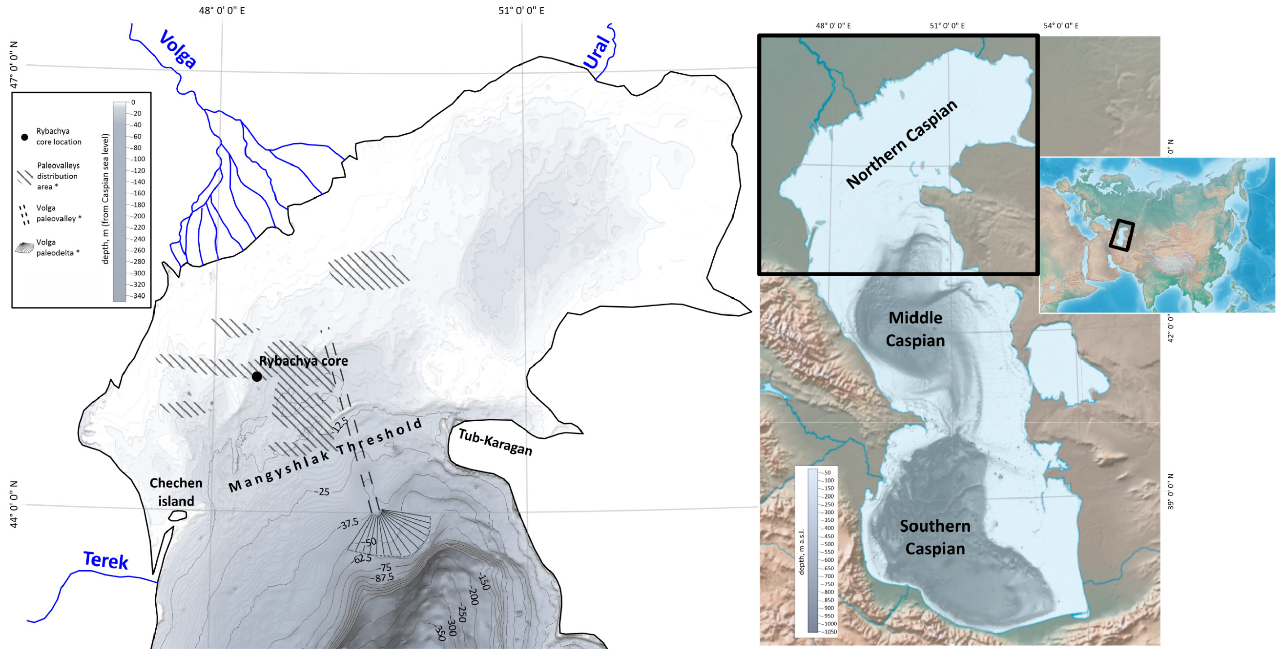
:1. Introduction

2. Materials and Methods
2.1. Grain Size Analysis
2.2. Geochemical Analyses
2.3. Mollusk Fauna Analysis
2.4. Diatom Analysis
2.5. Ostracod Analysis
2.6. Radiocarbon Dating
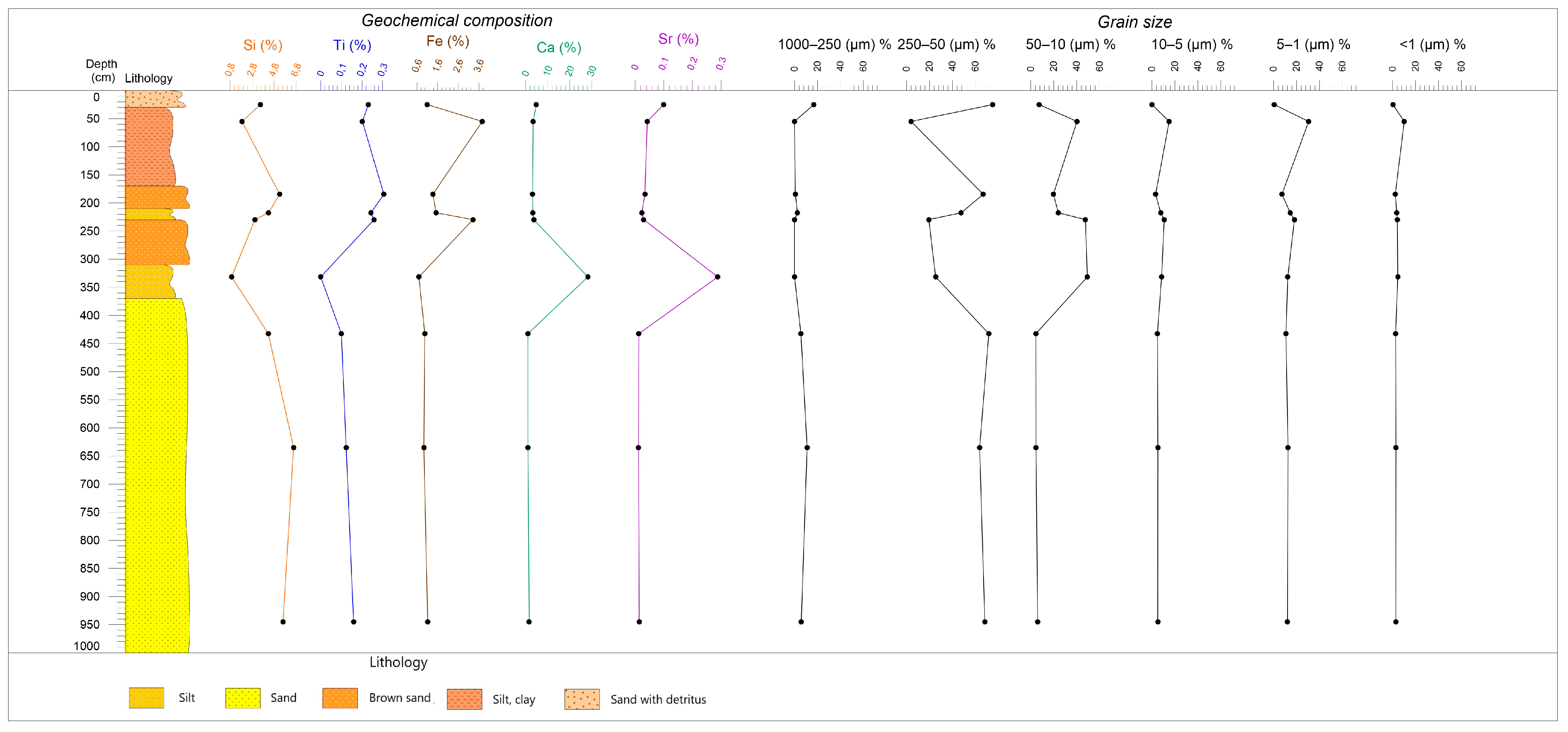
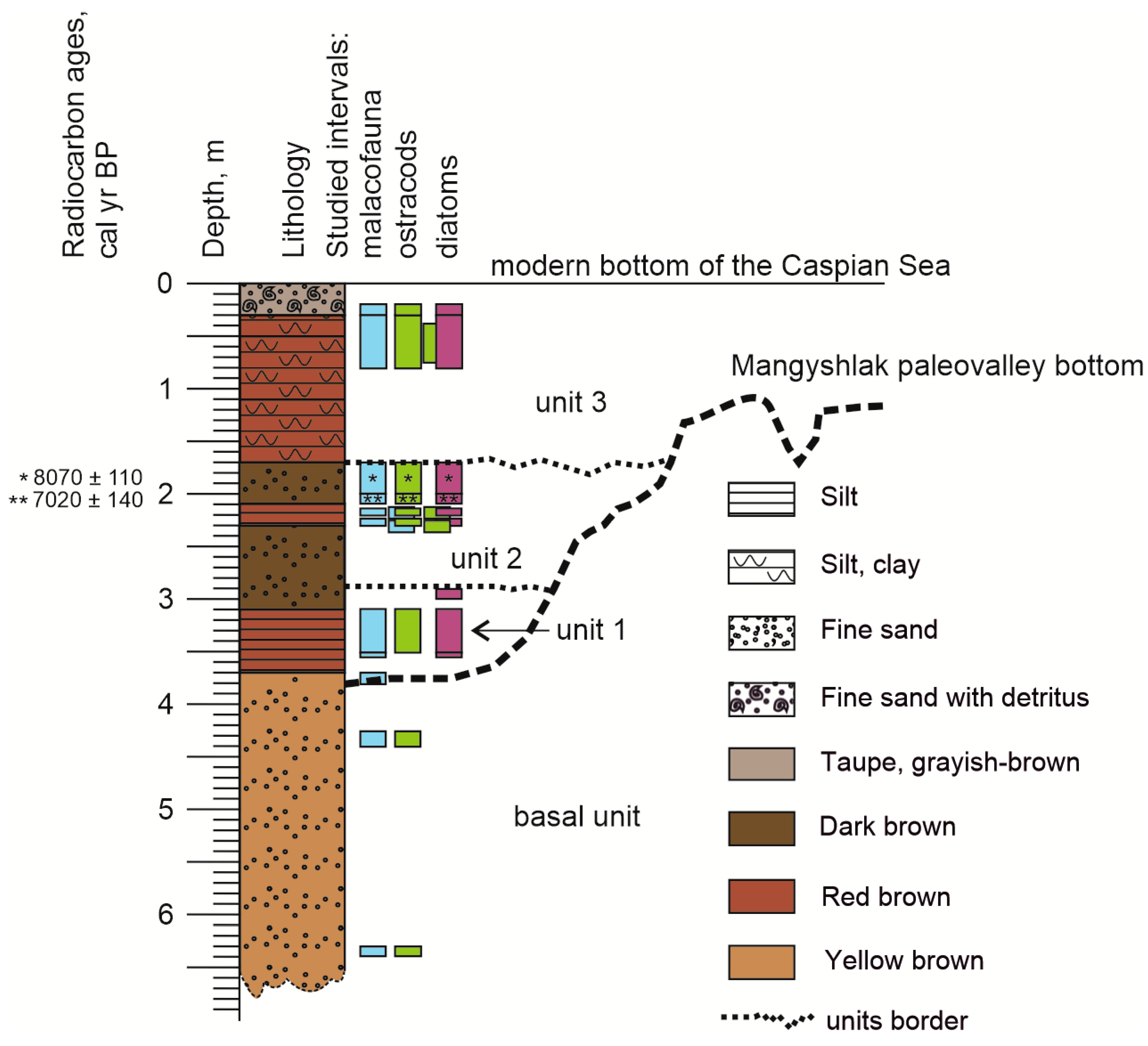
3. Results
3.1. Grain Size Analysis

3.2. Geochemical Analysis

| Depth (m) | Si (%) | Ti (%) | Fe (%) | Ca (%) | Sr (%) | Other Elements (%) |
|---|---|---|---|---|---|---|
| 0.2–0.3 | 3.55 | 0.23 | 1.10 | 4.80 | 0.10 | 90.23 |
| 0.3–0.8 | 1.90 | 0.20 | 3.76 | 3.40 | 0.04 | 90.70 |
| 1.73–1.96 | 5.30 | 0.31 | 1.37 | 3.14 | 0.03 | 89.85 |
| 2.15–2.20 | 4.30 | 0.24 | 1.53 | 3.25 | 0.02 | 90.65 |
| 2.35–2.34 | 3.06 | 0.26 | 3.31 | 3.68 | 0.03 | 89.66 |
| 3.13–3.50 | 0.95 | 0.00 | 0.69 | 28.20 | 0.29 | 69.87 |
| 4.25–4.40 | 4.28 | 0.10 | 0.98 | 1.01 | 0.01 | 93.62 |
| 6.3–6.4 | 6.57 | 0.12 | 0.93 | 1.03 | 0.01 | 91.33 |
| 9.40–9.50 | 5.61 | 0.16 | 1.12 | 1.58 | 0.01 | 91.52 |
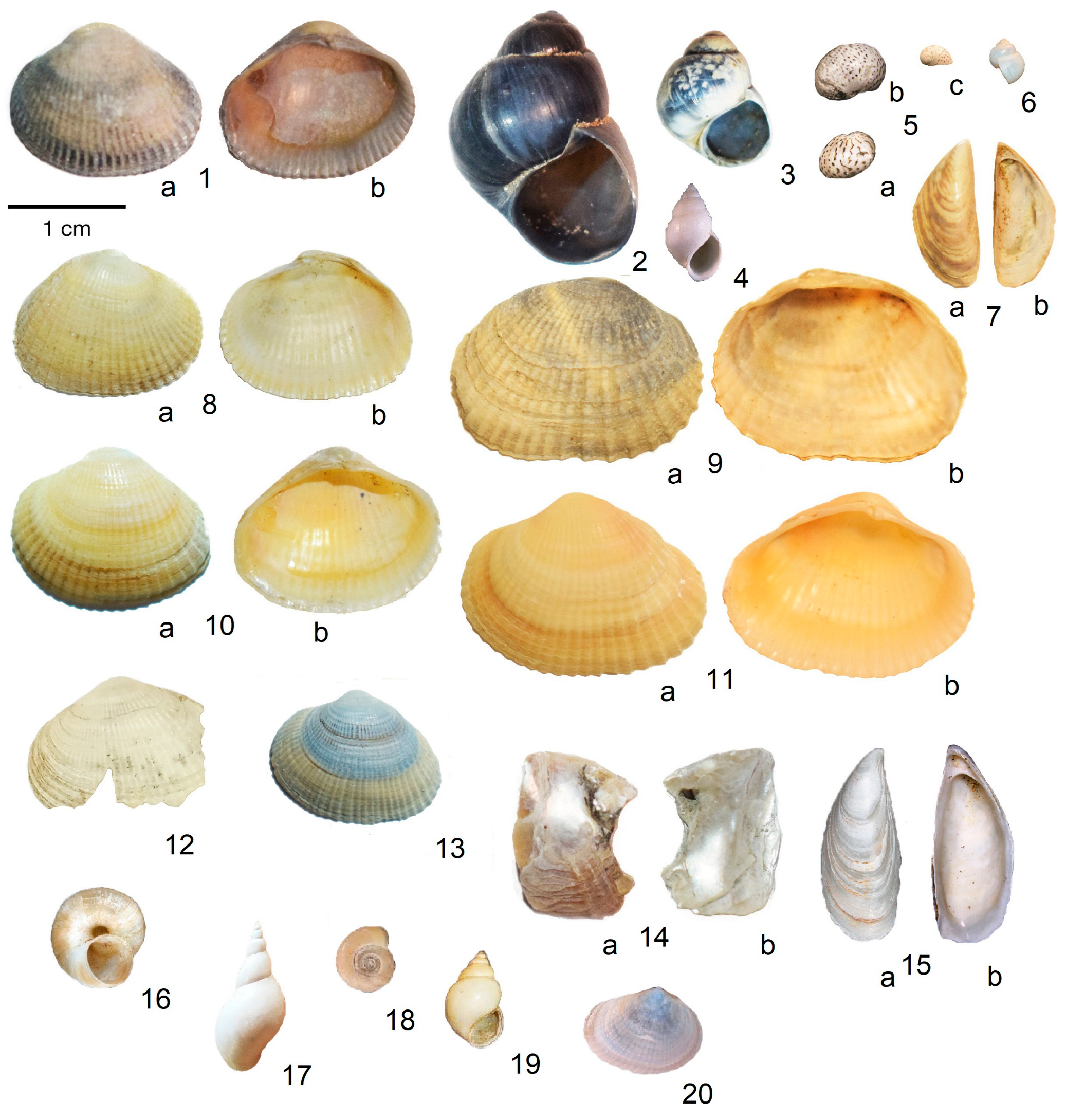
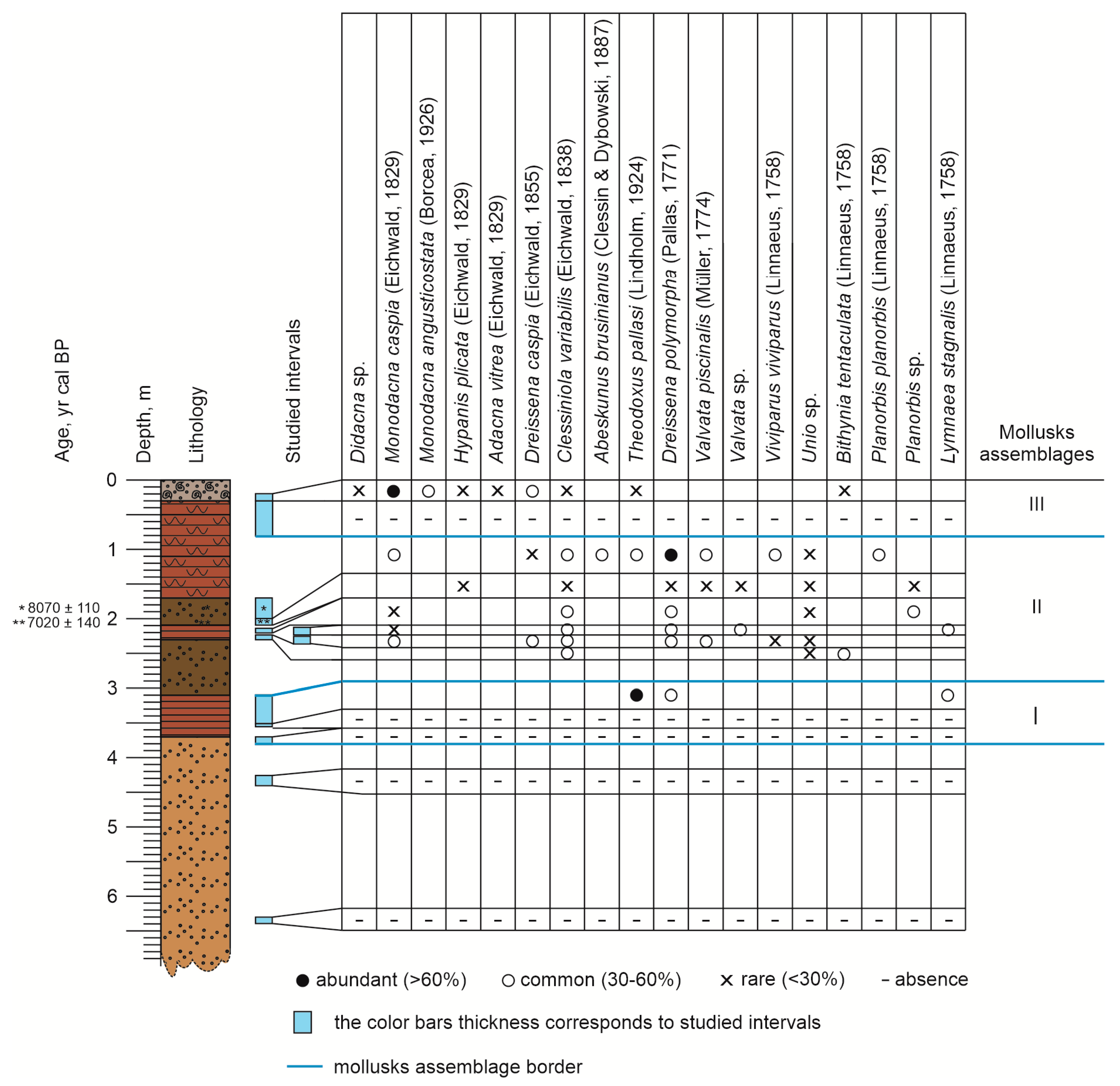
3.3. Mollusk Fauna


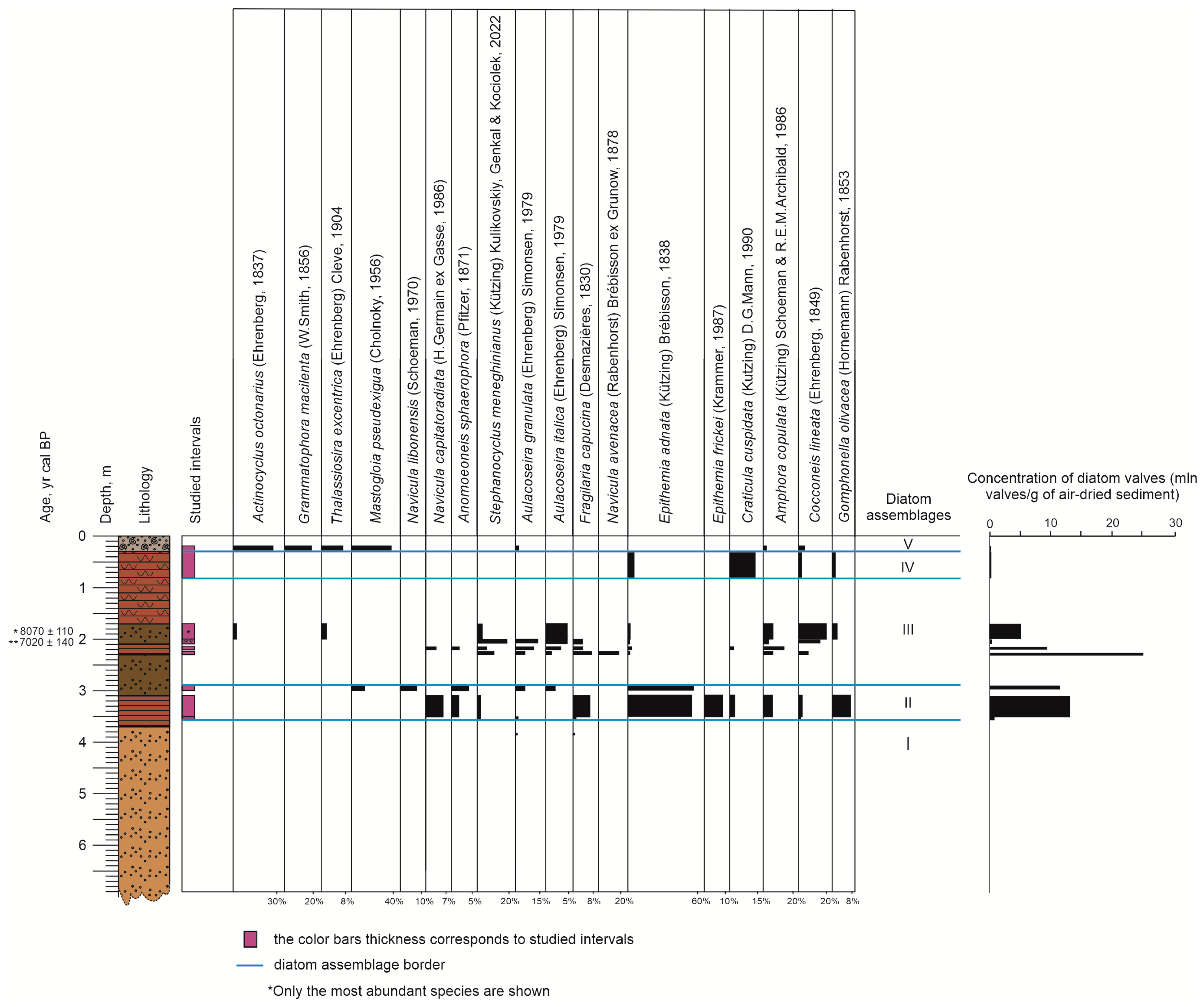
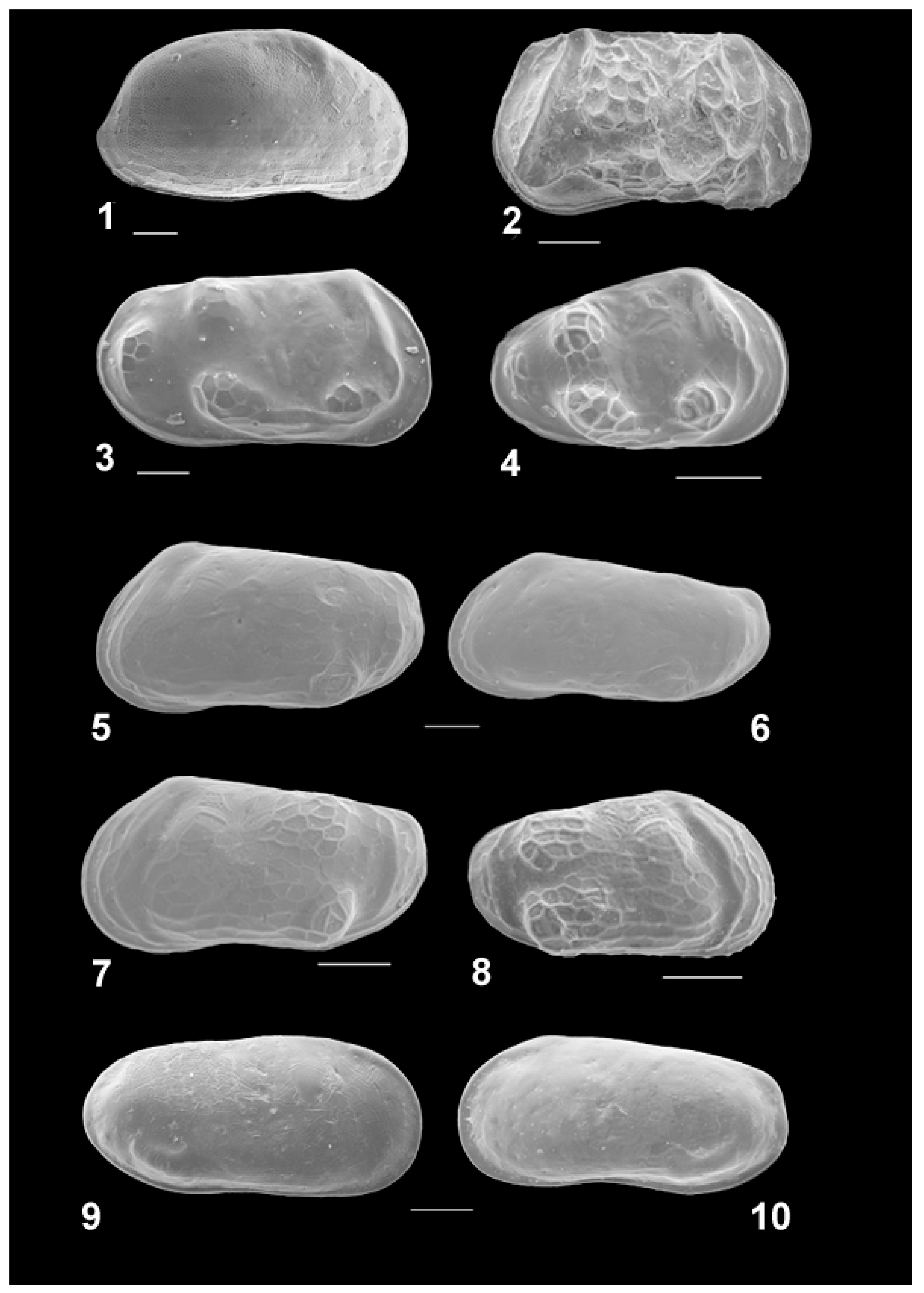
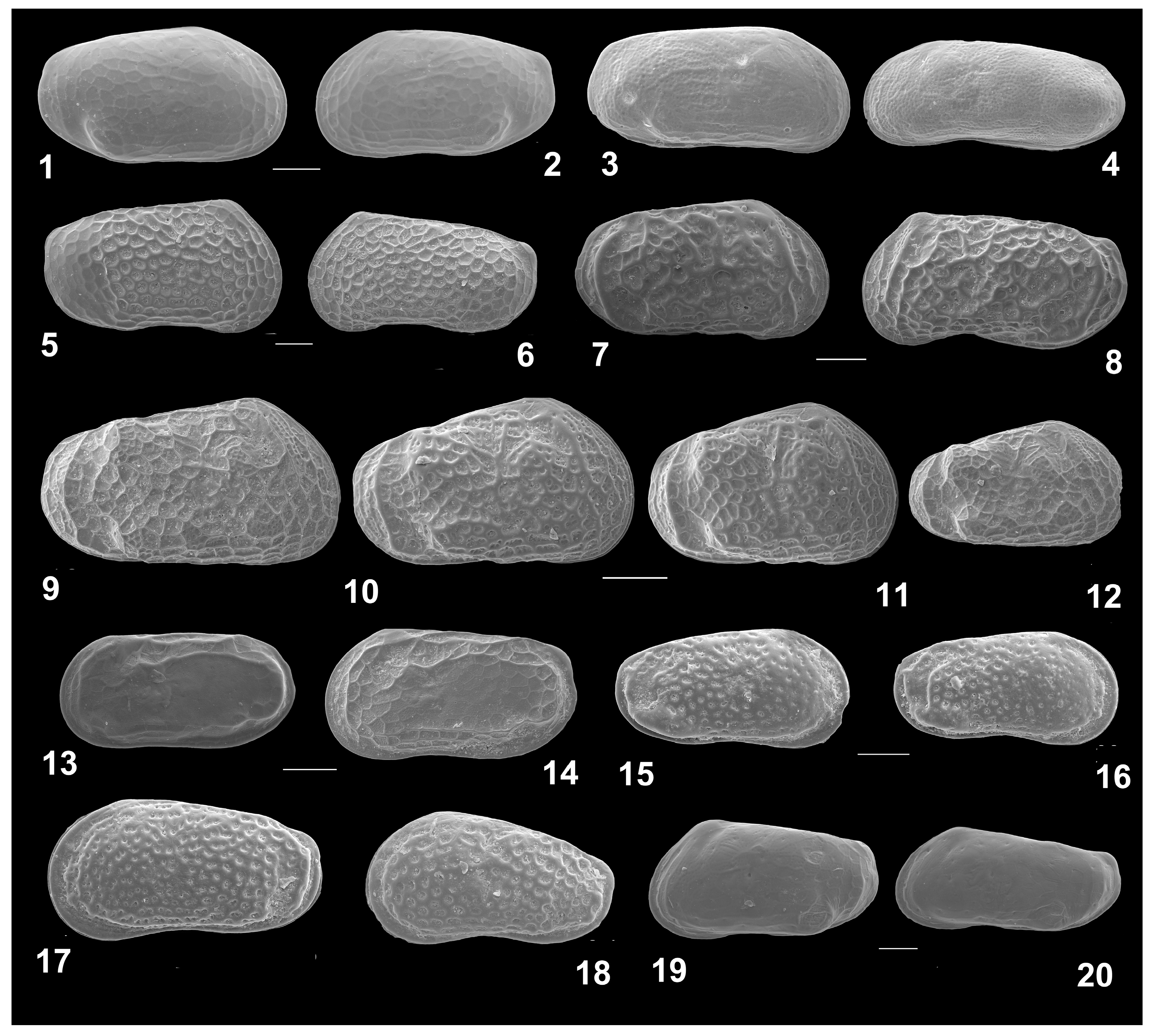
3.4. Diatoms


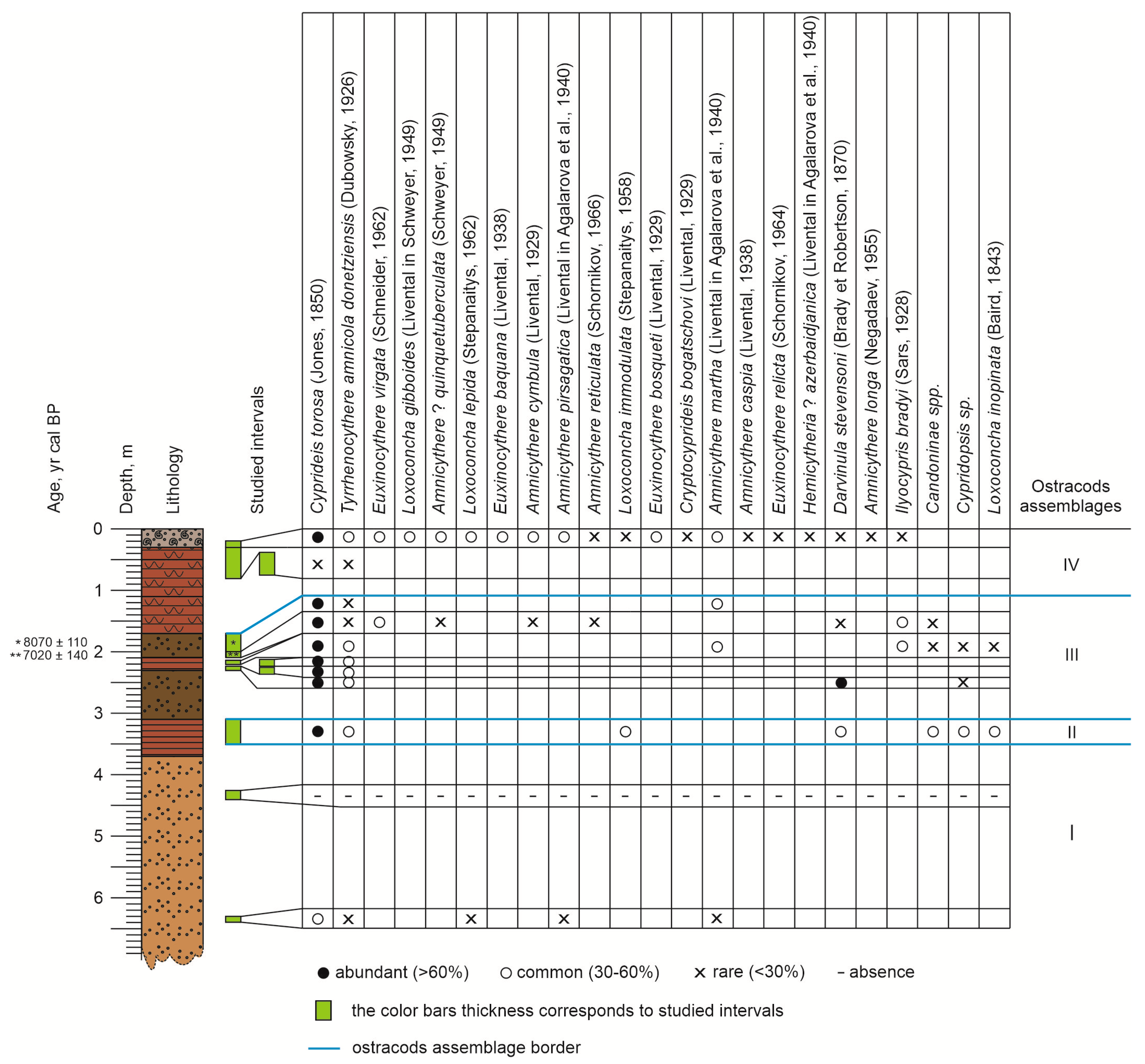
3.5. Ostracods


3.6. Radiocarbon Dating
4. Discussion
5. Conclusions
Author Contributions
Funding
Institutional Review Board Statement
Informed Consent Statement
Data Availability Statement
Acknowledgments
Conflicts of Interest
References
- Yanina, T.A.; Bolikhovskaya, N.S.; Sorokin, V.M.; Berdnikova, A.A.; Tkach, N.T. Paleogeography of the Caspian Sea in the Late Pleistocene—Holocene. In Actual Problems of the Pleistocene Paleogeography. Scientific Achievements of the School of Academician K.K. Markov; Yanina, T.A., Bolikhovskaya, N.S., Polyakova, Y.I., Klyuvitkina, T.S., Kurbanov, R.N., Eds.; Faculty of Geography, Moscow State University: Moscow, Russia, 2020; pp. 317–365. [Google Scholar]
- Zonn, I.S. The Caspian Encyclopedia; International Relations Publ.: Moscow, Russia, 2004; pp. 1–461. [Google Scholar]
- Kostianoy, A.G.; Kosarev, A.N. The Caspian Sea Environment; Springer: Berlin/Heidelberg, Germany, 2005; pp. 1–268. [Google Scholar] [CrossRef]
- Sidorchuk, A.Y.; Panin, A.V.; Borisova, O.K. Morphology of river channels and surface runoff in the Volga River basin (East European Plain) during the Late Glacial period. Geomorphology. 2009, 113, 137–157. [Google Scholar] [CrossRef]
- Panin, A.V.; Sidorchuk, A.Y.; Ukraintsev, V.Y. The Contribution of Glacial Melt Water to Annual Runoff of River Volga in the Last Glacial Epoch. Water Resour. 2021, 48, 877–885. [Google Scholar] [CrossRef]
- Varushchenko, S.I.; Varushchenko, A.N.; Klige, R.K. Change of Regime of Caspian Sea and Drainless Water Bodies in Paleotime; Nauka: Moscow, Russia, 1987; 239p. [Google Scholar]
- Rychagov, G.I. Holocene oscillations of the Caspian Sea, and forecasts based on palaeogeographical reconstructions. Quat. Int. 1997, 41/42, 167–172. [Google Scholar] [CrossRef]
- Kislov, A.V.; Toropov, P.M. East European river runoff and Black Sea and Caspian Sea level changes as simulated within the Paleoclimate modeling intercomparison project. Quat. Int. 2007, 167–168, 40–48. [Google Scholar] [CrossRef]
- Svitoch, A.A. Khvalynian transgression of the Caspian Sea was not a result of water overflow from the Siberian Proglacial lakes, nor a prototype of the Noachian flood. Quat. Int. 2009, 197, 115–125. [Google Scholar] [CrossRef]
- Kislov, A.; Panin, A.V.; Toropov, P. Current status and palaeostages of the Caspian Sea as a potential evaluation tool for climate model simulations. Quat. Int. 2014, 345, 48–55. [Google Scholar] [CrossRef]
- Yanina, T.A. The Ponto–Caspian region: Environmental consequences of climate change during the Late Pleistocene. Quat. Int. 2014, 345, 88–99. [Google Scholar] [CrossRef]
- Koriche, S.A.; Singarayer, J.S.; Cloke, H.L.; Valdes, P.J.; Wesselingh, F.P.; Kroonenberg, S.B.; Wickert, A.D.; Yanina, T.A. What are the drivers of Caspian Sea level variation during the late Quaternary? Quat. Sci. Rev. 2022, 283, 107457. [Google Scholar] [CrossRef]
- Yanina, T.A. Didacnas of the Ponto–Caspian; Madzhenta Press: Moscow/Smolensk, Russia, 2005; pp. 1–300. [Google Scholar]
- Yanina, T.A. Neopleistocene of the Ponto–Caspian Region: Biostratigraphy, Paleogeography, Correlation; Lomonosov Moscow State University, Geographical Faculty: Moscow, Russia, 2012; pp. 1–264. [Google Scholar]
- Boomer, I.; von Grafenstein, U.; Guichard, F.; Bieda, S. Modern and Holocene sublittoral ostracod assemblages (Crustacea) from the Caspian Sea: A unique brackish, deep–water environment. Palaeogeogr. Palaeoclimatol. Palaeoecol. 2005, 225, 173–186. [Google Scholar] [CrossRef]
- Chekhovskaya, M.P.; Zenina, M.A.; Matul, A.G.; Stepanova, A.Y.; Rakovski, A.Z. Reconstruction Environmental Changes in the North Caspian Sea Shelf During the Holocene by Ostracoda. Oceanology 2018, 58, 89–101. [Google Scholar] [CrossRef]
- Leroy, S.A.G.; Lopez–Merino, L.; Kozina, N. Dinocyst records from deep cores reveal a reversed salinity gradient in the Caspian Sea at 8.5–4.0 cal ka BP. Quat. Sci. Rev. 2019, 209, 1–12. [Google Scholar] [CrossRef] [Green Version]
- Svitoch, A.A. Hierarchy and chronology of the Holocene oscillations of the Caspian Sea level. In Changes of the Natural Territorial Complexes in the Zones of Anthropogenic Impact; Media–Press: Moscow, Russia, 2006; pp. 125–132. [Google Scholar]
- Bezrodnykh, Y.P.; Sorokin, V.M. On the age of the Mangyshlak deposits of the northern Caspian Sea. Quat. R. 2016, 85, 245–254. [Google Scholar] [CrossRef]
- Svitoch, A.A.; Yanina, T.A. Quaternary Sediments of the Caspian Sea Coasts; Rosselchozakademiya: Moscow, Russia, 1997; pp. 1–267. [Google Scholar]
- Zastrozhnov, A.S.; Danukalova, G.A.; Shick, S.M.; van Kolfshoten, T. State of stratigraphic knowledge of Quaternary deposits in European Russia: Unresolved issues and challenges for further research. Quat. Int. 2018, 478, 1–26. [Google Scholar] [CrossRef]
- Krijgsman, W.; Tesakov, A.; Yanina, T.; Lazarev, S.; Danukalova, G.; Van Baak, C.G.; Agustí, J.; Alçiçek, M.C.; Aliyeva, E.; Bista, D.; et al. Quaternary time scales for the Pontocaspian domain: Interbasinal connectivity and faunal evolution. Earth Sci. Rev. 2019, 188, 1–40. [Google Scholar] [CrossRef]
- Kroonenberg, S.B.; Abdurakhmanov, G.M.; Badyukova, E.V.; Van der Borg, K.; Kalashnikov, A.; Kasimov, N.S.; Rychagov, G.I.; Svitoch, A.A.; Vonhof, H.B.; Wesselingh, F.P. Solar–forced 2600 BP and Little ice age highstands of the Caspian sea. Quat. Int. 2007, 173–174, 137–143. [Google Scholar] [CrossRef] [Green Version]
- Richards, K.; Mudie, P.; Rochon, A.; Athersuch, J.; Bolikhovskaya, N.; Hoogendoorn, R.; Verlinden, V. Late Pleistocene to Holocene evolution of the Emba delta, Kazakhstan, and coastline of the north–eastern Caspian Sea: Sediment, ostracods, pollen and dinoflagellate cyst records. Palaeogeogr. Palaeoclimatol. Palaeoecol. 2017, 468, 427–452. [Google Scholar] [CrossRef]
- Fedorov, P.V. Stratigraphy of Quarternary Deposits and History of Development of the Caspian Sea; Trudy of the Geological Institute of the Academy of Science, Nauka: Moscow, Russia, 1957; Volume 10, pp. 1–308. [Google Scholar]
- Andrusov, N.I. Sketch about development of the Caspian Sea and its inhabitants. Izv. Russ. Geogr. Soc. 1888, 2, 91–114. [Google Scholar]
- Eichwald, E. Faunae Caspii maris primitae. Bull. De La Société Impériale Des Nat. De Moscou 1838, II, 125–174. [Google Scholar]
- Pravoslavlev, P.A. Caspian deposits of the Ural River. Izv. Don. Polytechn. Inst. 1913, 2, 1–60. [Google Scholar]
- Bogachev, V.V. Geological observations in the Manych valley, made in the summer of 1903. Izv. Geol. Komissii 1903, 22, 73–162. [Google Scholar]
- Bezrodnykh, Y.P.; Romanyuk, B.F.; Deliya, S.V.; Magomedov, R.D.; Sorokin, V.M.; Parunin, O.B.; Babak, E.V. Biostratigraphy and structure of the Upper Quaternary deposits and some paleogeographic features of the north Caspian region. Stratigr. Geol. Corr. 2004, 12, 102–120. [Google Scholar]
- Bezrodnykh, Y.P.; Deliya, S.V.; Romanyuk, B.F.; Sorokin, V.M.; Yanina, T.A. New data on the upper quaternary stratigraphy of the north Caspian sea. Dokl. Earth Sci. 2015, 462, 479–483. [Google Scholar] [CrossRef]
- Bezrodnykh, Y.; Yanina, T.; Sorokin, V.; Romanyuk, B. The Northern Caspian Sea: Consequences of climate change for level fluctuations during the Holocene. Quat. Int. 2020, 540, 68–77. [Google Scholar] [CrossRef]
- Rychagov, G.I. The sea-level regime of the Caspian Sea during the last 10,000 years. Bull. Mosc. State Univ. Ser. 5 1993, 2, 38–49. [Google Scholar]
- Kachinskiy, N.A. Soil Physics—Part 1; Higher Education Publishing House (USSR): Moscow, Russia, 1965; pp. 1–324. [Google Scholar]
- Rusakov, A.; Sedov, S. Late Quaternary pedogenesis in periglacial zone of northeastern Europe near ice margins since MIS 3: Timing, processes, and linkages to landscape evolution. Quat. Int. 2012, 265, 126–141. [Google Scholar] [CrossRef]
- Lebedeva, M.; Makeev, A.; Rusakov, A.; Romanis, T.; Yanina, T.; Kurbanov, R.; Kust, P.; Varlamov, E. Landscape dynamics in the caspian lowlands since the last deglaciation reconstructed from the pedosedimentary sequence of srednaya Akhtuba, southern Russia. Geosciences 2018, 8, 492. [Google Scholar] [CrossRef] [Green Version]
- Nevesskaja, L.A. History of the genus Didacna (Bivalvia: Cardiidae). Paleontol. J. 2007, 41, 861–949. [Google Scholar] [CrossRef]
- Smol, J.P.; Birks, H.J.; Last, W.M. Tracking Environmental Change Using Lake Sediments: Terrestrial, Algal and Siliceous Indicators; Kluwer Academic Publishers: Alphen aan den Rijn, The Netherlands, 2001; pp. 1–327. [Google Scholar]
- Krammer, K.; Lange–Bertalot, H. Bacillariophyceae. 1. Teil: Naviculaceae. In Süsswasserflora von Mitteleuropa; Ettl, H., Gerloff, J., Heynig, H., Mollenhauer, D., Eds.; Fisher Verlag: Jena, Germany, 1986; Volume 2, pp. 1–976. [Google Scholar]
- Krammer, K.; Lange–Bertalot, H. Bacillariophyceae. 2. Teil: Bacillariaceae, Epithemiaceae, Surirellaceae. In Süsswasserflora von Mitteleuropa; Ettl, H., Gerloff, J., Heynig, H., Mollenhauer, D., Eds.; Fisher Verlag: Stuttgart, Germany, 1988; Volume 2, pp. 1–596. [Google Scholar]
- Krammer, K.; Lange–Bertalot, H. Bacillariophyceae. 3. Teil: Centrales, Fragilariaceae, Eunotiaceae. In Süsswasserflora von Mitteleuropa; Ettl, H., Gerloff, J., Heynig, H., Mollenhauer, D., Eds.; Fisher Verlag: Jena, Germany, 1991; Volume 2, pp. 1–576. [Google Scholar]
- Krammer, K.; Lange–Bertalot, H. Bacillariophyceae. 4. Teil: Achnanthaceae. Kritische Ergänzungen zu Navicula (Lineolatae) und Gomphonema. In Süsswasserflora von Mitteleuropa; Ettl, H., Gerloff, J., Heynig, H., Mollenhauer, D., Eds.; Fisher Verlag: Jena, Germany, 1991; Volume 2, pp. 1–437. [Google Scholar]
- Zabelina, M.M.; Kiselev, I.A.; Proshkina–Lavrenko, A.I.; Sheshukova, V.S. Key to the Freshwater Algae of the USSR. Iss. 4. Diatoms; Nauka: Moscow, Russia, 1951; pp. 1–619. [Google Scholar]
- Ivanova, E.V.; Marret, F.; Zenina, M.A.; Murdmaa, I.O.; Chepalyga, A.L.; Bradley, L.R.; Schornikov, E.I.; Levchenko, O.V.; Zyryanova, M.I. The Holocene Black Sea reconnection to the Mediterranean Sea: New insights from the northeastern Caucasian shelf. Palaeogeogr. Palaeoclim. Palaeoecol. 2015, 427, 41–61. [Google Scholar] [CrossRef]
- Zenina, M.A.; Ivanova, E.V.; Bradley, L.R.; Murdmaa, I.O.; Schornikov, E.I.; Marret, F. Origin, migration pathways, and paleoenvironmental significance of Holocene ostracod records from the northeastern Black Sea shelf. Quat. Res. 2017, 87, 49–65. [Google Scholar] [CrossRef] [Green Version]
- Zastrozhnov, A.; Danukalova, G.; Golovachev, M.; Osipova, E.; Kurmanov, R.; Zenina, M.; Zastrozhnov, D.; Kovalchuk, O.; Yakovlev, A.; Titov, V.; et al. Pleistocene palaeoenvironments in the Lower Volga region (Russia): Insights from a comprehensive biostratigraphical study of the Seroglazovka locality. Quat. Int. 2021, 590, 85–121. [Google Scholar] [CrossRef]
- Agalarova, D.A.; Kadyrova, Z.K.; Kulieva, S.A. Ostracoda from Pliocene and Post–Pliocene Deposits of Azerbaijan; Azerbaijan State: Baku, Azerbaijan, 1961; pp. 1–419. [Google Scholar]
- Mandelstam, M.I.; Markova, L.; Rosyeva, T.; Stepanaitys, N. Ostracoda of the Pliocene and Post–Pliocene Deposits of Turkmenistan; Turkmenistan Geological Institute: Ashkhabad, Turkmenistan, 1962; pp. 1–288. [Google Scholar]
- Karmishina, G.I. Pliocene Ostracoda from the Southern European Part of the USSR; Izdatelstvo Saratovskogo Universiteta: Saratov, Russia, 1975; pp. 1–376. [Google Scholar]
- Arslanov, K.A.; Tertychnaya, T.V.; Chernov, S.B. Problems and methods of dating low–activity samples by liquid scintillation counting. Radiocarbon 1993, 35, 393–398. [Google Scholar] [CrossRef] [Green Version]
- Bronk Ramsey, C. Radiocarbon calibration and analysis of stratigraphy: The OxCal program. Radiocarbon 1995, 37, 425–430. [Google Scholar] [CrossRef] [Green Version]
- Reimer, P.J.; Austin, W.E.; Bard, E.; Bayliss, A.; Blackwell, P.G.; Ramsey, C.B.; Butzin, M.; Cheng, H.; Edwards, R.L.; Friedrich, M.; et al. The IntCal20 northern hemisphere radiocarbon age calibration curve (0–55 cal kBP). Radiocarbon 2020, 62, 725–757. [Google Scholar] [CrossRef]
- Karpytchev, Y.A. Reconstruction of Caspian Sea-level fluctuations: Radiocarbon dating coastal and bottom deposits. Radiocarbon 1993, 35, 409–420. [Google Scholar] [CrossRef] [Green Version]
- Kuzmin, Y.V.; Nevesskaya, L.A.; Krivonogov, S.K.; Burr, G.S. Apparent 14C ages of the ‘pre–bomb’ shells and correction values (R, ∆R) for Caspian and Aral seas (central Asia). Nuclear Instr. Meth. Phys. Res. 2007, 259, 463–466. [Google Scholar] [CrossRef]
- Gofman, E.F. Ecology of Modern and New Caspian Ostracods of the Caspian Sea; Nauka: Moscow, Russia, 1966; pp. 1–184. [Google Scholar]
- Borisova, O.K. Landscape and climatic changes in the Holocene. Izv. RAS Geogr. Ser. 2014, 2, 5–20. [Google Scholar] [CrossRef] [Green Version]
- Bolikhovskaya, N.S. Evolution of the climate and landscapes of the lower Volga region during Holocene. Vestnik Mos Unv. Ser. Geogr. 2011, 2, 13–27. [Google Scholar] [CrossRef]
- Richards, K.; Bolikhovskaya, N.; Hoogendoorn, R.; Kroonenberg, S.B.; Leroy, S.A.; Athersuch, J. Reconstructions of deltaic environments from Holocene palynological records in the Volga delta, northern Caspian Sea. Holocene 2014, 24, 1226–1252. [Google Scholar] [CrossRef] [Green Version]
- Alley, R.B.; Mayevski, P.A.; Sowers, T.; Stuiver, M.; Taylor, K.C.; Clark, P.U. Holocene climatic instability: A prominent, widespread event 8200 yr ago. Geology 1997, 25, 483–486. [Google Scholar] [CrossRef]
- Makshaev, R.R. Chemical composition of Lower Khvalynian deposits in the Middle and Lower Volga region. In Proceedings of the IGCP 610 and INQUA IFG POCAS, Palermo, Italy, 1–9 October 2017; pp. 118–120. [Google Scholar]
- Sudakova, N.G.; Nemtsova, G.M.; Andreicheva, L.N.; Bolshakov, V.A.; Glushankova, N.I. Lithology of the Middle Pleistocene tills in the central and southern Russian Plain. In Glacial Deposits in North–Eastern Europe; Ehlers, J., Kozarski, S., Gibbard, P., Eds.; Brookfield: Rotterdam, The Netherlands, 1995; pp. 181–189. [Google Scholar]
- Faustova, M.A.; Gribchenko, Y.N. Lithology of glacial deposits of the last Late Pleistocene glaciation. In Glacial Deposits in North–Eastern Europe; Ehlers, J., Kozarski, S., Gibbard, P., Eds.; Brookfield: Rotterdam, The Netherlands, 1995; pp. 194–199. [Google Scholar]
- Lobacheva, D.M.; Badyukova, E.N.; Makshaev, R.R. Lithofacial structure and conditions of accumulation of Baer knoll deposits in the Northern Caspian region. Vestnik Mosk. Univ. Ser. 5 Geogr. 2021, 6, 89–101. [Google Scholar]
- Zhai, D.; Xiao, J.; Fan, J.; Wen, R.; Pang, Q. Differential transport and preservation of the instars of Limnocythere inopinata (Crustacea, Ostracoda) in three large brackish lakes in northern China. Hydrobiologia 2014, 747, 1–18. [Google Scholar] [CrossRef]
- Kakroodi, A.A.; Leroy, S.A.G.; Kroonenberg, S.B.; Lahijani, H.A.K.; Alimohammadian, H.; Boomer, I.; Goorabi, A. Late Pleistocene and Holocene sea-level change and coastal paleoevironment evolution along the Iranian Caspian shore. Mar. Geol. 2015, 316, 111–125. [Google Scholar] [CrossRef]
- Leroy, S.A.G.; Lopes–Merio, L.; Tudryn, A.; Chalié, F.; Gasse, F. Late Pleistocene and Holocene palaeoenvironments in and around the middle Caspian basin as reconstructed from a deep–sea core. Quat. Sci. Rev. 2014, 1–20. [Google Scholar] [CrossRef] [Green Version]
- Wesselingh, F.P.; Neubauer, T.A.; Anistratenko, V.V.; Vinarski, M.V.; Yanina, T.; Poorten, J.J.; Kijashko, P.; Albrecht, C.; Anistratenko, O.Y.; D’Hont, A.; et al. Mollusc species from the Pontocaspian region—An expert opinion list. Zookeys 2019, 827, 31–124. [Google Scholar] [CrossRef] [Green Version]
- Neubauer, T.A.; van de Velde, S.; Yanina, T.A.; Wesselingh, F.P. A late Pleistocene gastropod fauna from the northern Caspian Sea with implications for Pontocaspian gastropod taxonomy. ZooKeys 2018, 770, 43–103. [Google Scholar] [CrossRef] [Green Version]
- Orlova, M.I.; Therriault, T.W.; Antonov, P.I.; Shcherbina, G.K. Invasion ecology of quagga mussels (Dreissena rostriformis bugensis): A review of evolutionary and phylogenetic impacts. Aquat. Ecol. 2005, 39, 401–418. [Google Scholar] [CrossRef]
- Smith, A.J.; Horne, J.H. Ecology of marine, marginal marine and nonmarine ostracods. In The Ostracoda. Applications in Quaternary Research; AGU: Washington, DC, USA, 2002; pp. 37–64. [Google Scholar] [CrossRef]
- Gandolfi, A.; Todeschi, E.B.A.; Rossi, V.; Menozzi, P. Life history traits in Darwinula stevensoni (Crustacea: Ostracoda) from Southern European populations under controlled conditions and their relationship with genetic features. J. Limnol. 2001, 60, 1–10. [Google Scholar] [CrossRef] [Green Version]
- van de Velde, S.; Yanina, T.A.; Neubauer, T.A.; Wesselingh, F.P. The Late Pleistocene mollusk fauna of Selitrennoye (Astrakhan province, Russia): A natural baseline for endemic Caspian Sea faunas. J. Great Lakes Res. 2019, 46, 1227–1239. [Google Scholar] [CrossRef]
- van de Velde, S.; Wesselingh, F.P.; Yanina, T.A.; Anistratenko, V.V.; Neubauer, T.A.; ter Poorten, J.J.; Vonhof, H.B.; Kroonenberg, S.B. Mollusc biodiversity in late Holocene nearshore environments of the Caspian Sea: A baseline for the current biodiversity crisis. Palaeogeogr. Palaeoclim. Palaeoec. 2019, 535, 109364. [Google Scholar] [CrossRef]
- Makshaev, R.R.; Svitoch, A.A.; Tkach, N.T. Late Pleistocene sedimentation in the Northern Caspian Lowland during the Early Khvalynian transgression. Limn. Freshw. Biol. 2020, 4, 531–532. [Google Scholar] [CrossRef]
- Velichko, A.A. Evolutionary Geography: Problems and Decisions; GEOS: Moscow, Russia, 2012; pp. 1–564. [Google Scholar]
- Novenko, E.Y. Changes of Vegetation and Climate Central and Eastern Europe in the Late Pleistocene and the Holocene in Interglacial and Transitional Stages of the Climatic Macrocycles. Ph.D. Dissertation, Moscow State University, Moscow, Russia, 2016; pp. 1–44. [Google Scholar]
- Arnoldi, L.I. On the question of the distribution of zoobenthos in the Caspian Sea. In Materials on Hydrobiology and Lithology of the Caspian Sea; Publishing House of the Academy of Sciences of the USSR: Moscow, Russia, 1938; pp. 115–171. [Google Scholar]
- Karpevich, A.F. Relation of some species of the family Cardiidae to the salt regime of the Northern Caspian. Dokl. Acad. Sci. USSR New Ser. 1946, 54, 73–75. [Google Scholar]
- Zhadin, V.I. Mollusks of Fresh and Brackish Waters of the USSR; Publishing House of the Academy of Sciences of the USSR: Moscow, Russia, 1952; pp. 1–376. [Google Scholar]
- Neiman, A.A. On the characteristics of the Cardiidae of the Northern Caspian. Zool. J. 1959, 38, 1891–1893. [Google Scholar]
- Shornikov, E.I. Questions of ecology of the Azov–Black Sea ostracods. Biol. Sea 1972, 26, 53–88. [Google Scholar]

Disclaimer/Publisher’s Note: The statements, opinions and data contained in all publications are solely those of the individual author(s) and contributor(s) and not of MDPI and/or the editor(s). MDPI and/or the editor(s) disclaim responsibility for any injury to people or property resulting from any ideas, methods, instructions or products referred to in the content. |
© 2023 by the authors. Licensee MDPI, Basel, Switzerland. This article is an open access article distributed under the terms and conditions of the Creative Commons Attribution (CC BY) license (https://creativecommons.org/licenses/by/4.0/).
Share and Cite
Berdnikova, A.; Lysenko, E.; Makshaev, R.; Zenina, M.; Yanina, T. Multidisciplinary Study of the Rybachya Core in the North Caspian Sea during the Holocene. Diversity 2023, 15, 150. https://doi.org/10.3390/d15020150
Berdnikova A, Lysenko E, Makshaev R, Zenina M, Yanina T. Multidisciplinary Study of the Rybachya Core in the North Caspian Sea during the Holocene. Diversity. 2023; 15(2):150. https://doi.org/10.3390/d15020150
Chicago/Turabian StyleBerdnikova, Alina, Elena Lysenko, Radik Makshaev, Maria Zenina, and Tamara Yanina. 2023. "Multidisciplinary Study of the Rybachya Core in the North Caspian Sea during the Holocene" Diversity 15, no. 2: 150. https://doi.org/10.3390/d15020150