Assessing the Spatiotemporal Relationship between Coastal Habitats and Fish Assemblages at Two Neotropical Estuaries of the Mexican Pacific

Abstract

Differences in fish assemblages’ structures and their relations with environmental variables (due to the variations in sampled seasons, habitats, and zones) were analyzed in two adjacent estuaries on the north Pacific coast of Mexico. Environmental variables and fish catches were registered monthly between August 2018 and October 2020. Multivariate analyses were conducted to define habitats and zones based on their environmental characteristics, and the effect of this variability on fish assemblages’ composition, biomass, and diversity (α and β) was evaluated. A total of 12,008 fish individuals of 143 species were collected using different fishing nets. Multivariate analyses indicated that fish assemblages’ structures were different between zones due to the presence, height, and coverage of distinct mangrove species. Additionally, depth and salinity showed effects on fish assemblages’ diversity (α and β-nestedness), which presented higher values in the ocean and remained similar in the rest of the analyzed zones and habitats. These results and the differences in species replacement (β-turnover) indicate the singularity of fish assemblages at estuaries (even in areas close to the ocean) and the necessity to establish local management strategies for these ecosystems.

1. Introduction

Wetland ecosystems play a crucial ecological role due to their high primary productivity and habitat complexity that promotes the presence of multiple species. High habitat complexity of wetlands comprehends heterogeneous structural features, such as mangrove forests, and exclusive physiochemical conditions [1,2] as a result of their location at the interface between freshwater input from rivers and saline water from the sea [3,4], which are mainly determined by waves, tidal regimes, river discharges, coastal currents circulation, and meteorological factors (winds and seasonal precipitation [5]). The fluctuation of environmental gradients and physical dynamics provide a suitable habitat for different fish species that live within wetlands during part or all of their life cycles [5,6,7,8,9,10], using them as nurseries, foraging sites, and refuge areas [11,12,13].

In addition, the habitat complexity in wetlands is due to the presence of mangrove forest structures (trees, shrubs, and prop roots) and tidal channels that connect the seaward edge of an estuary or coastal lagoon with the interior landward. These intricate complex networks protect coastal ecosystems from physical agents (storms and waves) and facilitate the migration of organisms within the shallow intertidal zone [14,15]. Thus, fish use wetlands during different life stages (juveniles and adults) as residents [16], in nurseries [17,18], or in transient habitats [19,20], which may influence spatial and temporal patterns of ichthyofauna’s assemblages.

Numerous studies have shown relationships between fish diversity and water conditions such as salinity [13,21], temperature, clarity [22,23], depth, and tidal ranges [24,25]. In tropical wetlands, spatial and seasonal fluctuations in salinity, temperature, and dissolved oxygen determine changes in fish densities and biomass [6,26]. Additional variables such as coastal geomorphology [27,28,29,30], nutrient cycles, and disturbance impacts [31] may also influence the fish distribution, abundance, and biomass.

The relative importance of the different factors influencing fish diversity in wetland ecosystems will vary, which does not necessarily mean that they will be mutually exclusive [11,29,32]. In this sense, the link between physical and biological interactions in wetlands could improve our understanding of ecological processes to propose informed management strategies [33]. However, community–environment studies are scarce for neotropical wetland ecosystems; thus, this study aimed to assess the relationship between fish assemblages and coastal habitats at two adjacent estuarine systems on the north Pacific coast of Mexico.

Even though both ecosystems have been studied previously on seasonal variations of environmental characteristics and fish community dynamics [31,34,35,36,37], there have not been any attempts to relate fish assemblages to specific habitats within each system. The wetland habitats were defined based on biotic and abiotic factors: mangrove cover and height, the extension of agricultural lands, salinity, water temperature, depth, climatic season, and the type of habitat (channel, mangrove creek, lagoon, river, and ocean). The working hypotheses are (A) the a priori designated habitats in both systems differ according to environmental characteristics; (B) fish diversity (α and β) and assemblages’ structure vary spatiotemporally according to habitat characteristics.

2. Materials and Methods

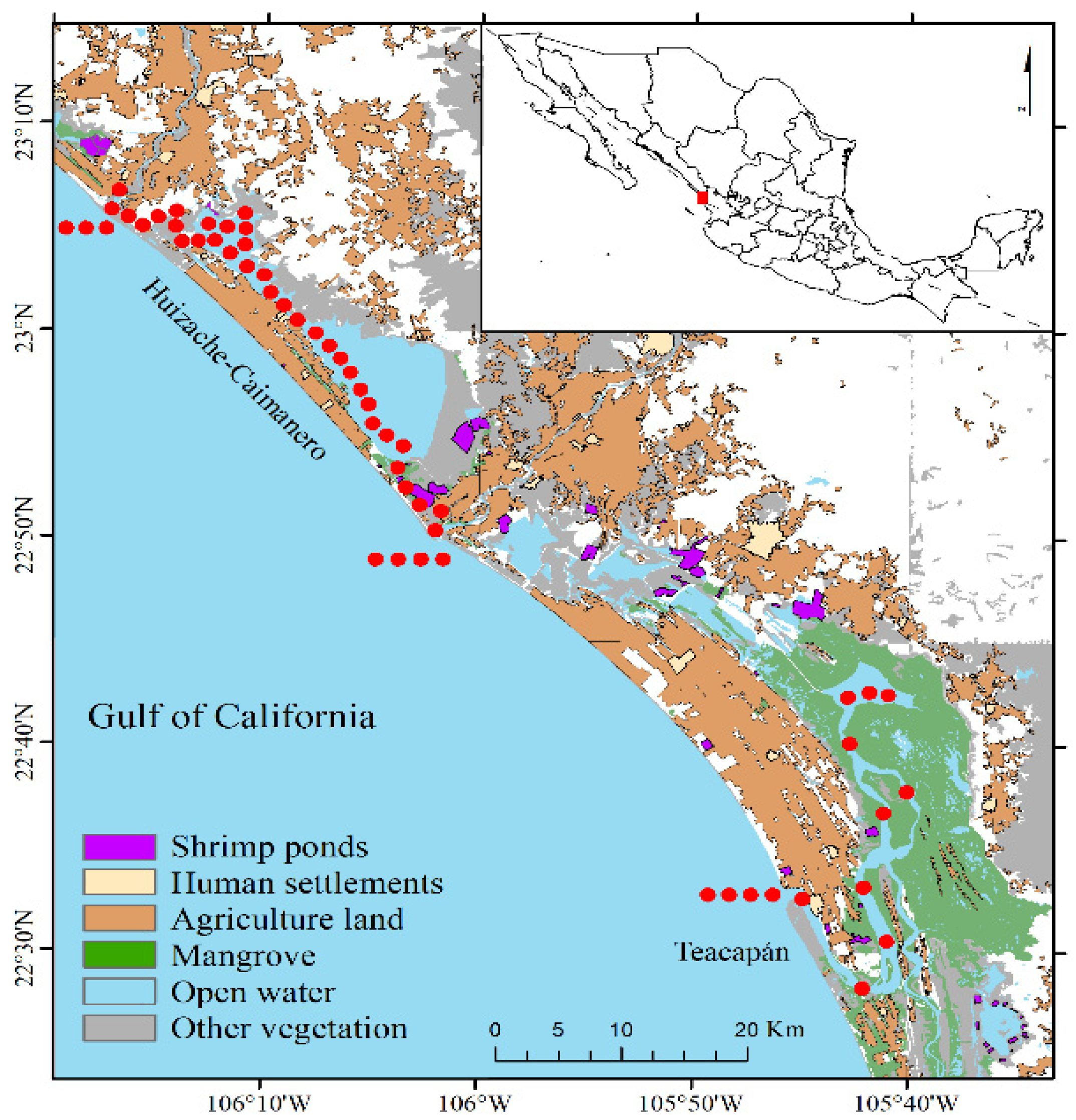
2.1. Study Area

The study was conducted in the estuarine systems of Huizache–Caimanero and Teacapan on the northeastern coast of Mexico (Figure 1). Huizache–Caimanero is a shallow intermittent estuary with a strong influence of freshwater inputs as it lies between two rivers (Presidio and Baluarte) that are connected to the coastal lagoons by narrow tidal channels surrounded by mangrove forest. This coastal system receives ample freshwater during the rainy season (June to November), which mixes with the seawater from the ocean, creating a typical estuarine circulation pattern. The average area of the coastal system is 175 km², reduced to 65 km² during the dry season. This ecosystem was designated Ramsar site in 2007 (no. 1689) to protect particular species (e.g., birds, fish, mammals, reptiles, amphibians, and invertebrates) and habitats such as mangrove forests. Teacapan is a tide-dominated estuary with high mangrove density and tall mangrove trees [31]. It has a 1 km long inlet with a depth of 9 m that connects the system with the Pacific Ocean. One river drains into the Teacapan system all year round (Cañas) and presents the main water body, Laguna Agua Grande, in the north section. This ecosystem is part of the Biosphere Reserve Marismas Nacionales, a Marine Protected Area established in 2010 to conserve a massive estuarine complex with the largest mangrove forest in the Mexican Pacific.

For this study, we divided the two coastal systems into seasons (DCS: dry-cold season, DWS: dry-warm season, RWS: rainy-warm season [31]), habitat, and zones according to geomorphic and biotic characteristics. The habitats are characterized as (i) Ocean: represents the main inlets of coastal systems with a direct connection with the Pacific Ocean up to depths of 20 m, which present effects of littoral currents, tidal forces, and waves from local wind and previous storms. (ii) Lagoons: described as the main water body of Huizache and Caimanero on the north, and Agua Grande lagoon nearby Teacapan. The Huizache and Caimanero coastal lagoons are part of the same wetland system with a geomorphic separation by a barrier in a narrow zone impeding the free transit of fish and other species through it. Moreover, this wetland does not present a mangrove community within the fringe zone of the main water body. In contrast, the Agua Grande lagoon within the Teacapan estuarine system presents a mangrove forest with large fringe trees of red mangrove Rhizophora mangle. (iii) Main tidal channel: corresponds to a wide geomorphic corridor that connects the ocean with the wetland systems. It is strongly influenced by the intense (1.4 m tide range) semidiurnal tidal cycle of the Pacific Ocean (two high and two low tides every lunar day). (iv) Inner tidal channel: stands for the principal water exchange route between the main tidal channel and the coastal lagoons, where extensive fringe mangrove forests thrive at the interface between water and land. Due to their geomorphic characteristics, the strong tidal currents from the Pacific Ocean attenuated within these zones. (v) Tidal mangrove creek: corresponds to the narrow water connections within the mangrove fringe community. These habitats are typically shallow and depict depressions at the interface between land and water. Due to the dense mangrove root configuration within these zones, mangroves function as refuges by juvenile fish and crustaceans. (vi) River: describes the streams of freshwater flowing in a meander geomorphic arrangement to the main inlet, thus presenting low salinity and less ocean influence.

The zones were assigned upon a visual inspection throughout the edge of the estuarine systems to establish the predominant vegetation at every sampling station, and these were classified as (i) Buttonwood mangrove (Conocarpus erectus), (ii) White mangrove (Laguncularia racemosa), (iii) Red mangrove (R. mangle), (iv) Unvegetated zones, and (v) Ocean.

2.2. Sampling Design and Procedures

A net of stations was placed at both systems covering all the different habitats (Figure 1); at each station, the date, salinity (‰), temperature (°C), and depth (m) were recorded with a Horiba U-50 Series multiparameter water quality checker. The mangrove height was estimated using a portable Vertex Laser VL400 hypsometer, while the mangrove and agricultural land extension was estimated using vectors over freely available Google Earth images recorded as close as possible to the field campaign date. Given the distance between sampling stations, a constant vector extension of 200 m coastline in front of it, was used to quantify the total cover area further inland. These data were used to construct the environmental matrix, including biotic and abiotic characterization of each sampling station.

The fish were collected during morning hours and at high tide from August 2018 to October 2020 at monthly intervals. At both estuarine systems, gillnets (mesh size = 2.5, 3, and 3.5 inches) were left adrift in each station (45 min), where the depth was over 1.5 m, while cast nets (mesh size = 0.6 inches) were deployed at stations where the depth was below 1.5 m. The fish organisms caught were placed in separate labeled plastic bags and transported in an icebox. Once in the laboratory, the fish identification was conducted in the lowest taxonomic category possible [38,39]. Each fish specimen was measured for the total length (mm) and body mass (g) to the nearest 1 mm and 0.1 g, respectively.

2.3. Data Analysis Environmental Data and Habitat Characteristics

A mean value was obtained for water temperature (°C) and salinity (ppt) for every climatic season, while a mean depth value (m) was determined for every habitat. Mean differences in water temperature and salinity were tested for every season using a one-way ANOVA with the season as a fixed factor. Before the analyses, homogeneity of variances was tested with Cochran’s C test. A posteriori pairwise means comparisons were made by running Tukey’s HSD test.

Spatiotemporal variations in environmental parameters (salinity, water temperature, depth, mangrove area and height, and extension of agricultural lands) were analyzed using multivariate analyses according to different factors (system, season, habitat, and zone) to determine if statistical differences existed among zones due to their environmental characteristics and if this has an effect on fish assemblages’ structure.

A matrix was constructed using each station as columns, and each haul-specific environmental parameter data constituted the rows. Data were normalized (mean of 0 and standard deviation of 1) given that the environmental values had different scales. Pearson’s correlation coefficients were used to determine statistically significant correlations between environmental variables. When a significant correlation was found, data were square-root or fourth-root transformed, and the previous analysis was rerun until the correlation was not significant. We used Excel’s regression tool to calculate Pearson’s correlation coefficients and their respective P-values. Subsequently, a similarity matrix of the standardized and transformed environmental data was constructed using Euclidian distance.

Factors were assigned to each station (estuarine system, climatic season, habitat, and zone), and a PERMANOVA [40] was performed to test the H₀: sampled stations were not different despite dissimilarities between the analyzed factors. If a p-value was <0.05, the H₀ was rejected, and then pairwise tests were performed to determine which stations were different. Due to the increased risk of inflated type I error (i.e., rejecting the null hypothesis when it is true), we applied a Bonferroni procedure by dividing α (0.05) by the number of comparisons.

Principal coordinates analysis (PCoA) was used to visualize the patterns of environmental data between the sampled stations and to determine which characteristics best explained the group separation where the PERMANOVA revealed statistical differences. This ordination method produces a two-dimensional scatter plot, and the characteristics of each station are overlaid as vectors. The trajectory of the vector indicates the importance of each environmental characteristic between sampling stations. Both axes have a scale from −n to n, in which the point 0.0 is the centroid meaning the location where all the points would be located if the null hypothesis was true [41].

2.4. Fish Assemblages

Biomass species composition data was used to determine the similarity degree in fish assemblages according to the assigned factors (estuarine system, climatic season, habitat, and zone) and their relationship to the environmental factors registered in the study area. Since different sampling methods were used, the species biomass data of each haul was standardized as Catch Per Unit Effort (CPUE), where the effort is defined as area [42], which represents the biomass of individuals in square kilometers for each species (i.e., g/km²). The catch area was calculated based on the gear type, a circle for the cast net, and a rectangle for the gillnet.

Specifically for the gillnet, the swept area was estimated using a GPS in every fishing operation to determine the beginning and end of the towed area. In addition, using central tendencies and dispersion of the gillnet, the data were bootstrapped approximately 2000 times until a normal distribution was fitted, and then standardized for N (μ,σ²)/ΣN (μ,σ²) where N is the normal distribution, μ is the population mean, and σ² is the population variance. Finally, an integration of the error was generated by bootstrapping the swept area by the gillnet and the total area towed with both fishing gears, so a CPUE was obtained in terms of the area for each haul.

Randomized species accumulation plots were constructed per estuarine system to assess the representativeness of the sampling effort. The samples were randomized 1000 times for each new cumulative species sample using Chao’s 1 estimator of the absolute number of species in an assemblage. This method is based on the number of rare species found in a sample [43], and the notation is:

$$S_{est}=S_{obs}+\left(\frac{f_1^2}{2f_2}\right)$$

where S_est is the estimated number of species, S_obs is the observed number of species in the sample, f₁ is the number of singletons (taxa represented by a single occurrence in the field campaign), and f₂ is the number of doubletons (two occurrences in the field campaign [44].

In order to explain the spatiotemporal differences in fish assemblages, a hierarchical analysis was performed using the following levels: estuarine system, climatic season, habitat, and zone. Differences in fish assemblages among these factors were tested using multivariate analyses. A matrix containing i lines (species), and j columns (hauls), was created and from this, a Bray-Curtis similarity matrix was generated using the mentioned levels, where each zone was considered a replicate within each habitat.

To test the H₀ that the fish assemblages did not differ according to these factors, a PERMANOVA was used with a fixed factor (model type I), and its statistical significance was tested using a type III sum of squares, with 10,000 unrestricted permutations of raw data [40]. The PERMDISP routine on PRIMER 7 (PRIMER-E, serial no. 7875) was conducted with a permutation test to examine the homogeneity of species composition between factors. Pairwise tests were performed to determine if estuarine systems, climatic seasons, habitats, and zones differed from the others, and a Bonferroni procedure was applied to correct multiple comparisons.

Additionally, a distance-based linear model permutation test (DistLM) was performed to examine the significance of each environmental variable contributing to the fish assemblages’ differences [45,46]. This analysis identified environmental variables that predict the variation in fish assemblages at the different estuarine systems, climatic seasons, habitats, and zones and represents it in multivariate space. DistLM did a partitioning of the variation in the data and showed it as a resemblance matrix calculated by multiple regression models [46]. A marginal test first showed the amount of variation explained by each variable when taken alone (ignoring the other variables), and then a sequential test (forward direction) allowed to select individual variables based on the Akaike information criterion (AIC) and the Bayesian information criterion (BIC) values. This step allowed to identify the parsimonious model representing the best combination of environmental variables that explained fish assemblages’ composition, and the proportion of explained variation attributed to each variable added to the model as a function of the other variables already present [40]. Based on the parsimonious model selected, a distance-based redundancy analysis (dbRDA) was conducted to visualize the relationship between fish assemblages’ composition and environmental variables. The assumption required by DISTLM analysis (the number of samples was higher than the number of variables) was met [40].

A similarity of percentage analysis (SIMPER, Bray–Curtis index, and cutoff at 90%) was used to determine the contribution of species to the average resemblance among the analyzed factors (estuarine system, climatic season, habitat, and zone [47]). Upon the identification of factors that contribute to the observed differences, α-diversity indices were computed based on haul-specific species biomass data standardized by the CPUE. Specifically, we used Hill numbers (i.e., effective numbers of species, ^qD), which have been recognized as the most appropriate method for evaluating diversity [48,49,50]. The indices used were ⁰D (species richness; gives disproportionate weight to rare species because is not sensitive to species biomass [48]), ¹D (exponential of Shannon’s entropy; the number of common species in the community as it weights each species according to its biomass in the sample [50]), and ²D (inverse Simpson concentration; the number of dominant species in the community as it favors species that present high biomass [50]). Formulas of the Hill numbers have already been extensively detailed [48,50]. Finally, the biomass per species matrix was transformed to presence/absence to calculate the local contribution of each sample to both components of β-diversity (turnover and nestedness), using the Sorensen dissimilarity coefficient.

Biomass, Hill numbers (⁰D, ¹D, and ²D), and β-diversity components (turnover and nestedness) calculated per haul were used as response variables in additive generalized models (GAMs), while explanatory variables were the environmental factors that presented an effect on fish assemblages according to the previous multivariate analyses. GAMs replace the linear form Σβ_jX_j with a sum of smooth functions ΣS_j(X_j), where the S_j()’s are unspecified functions that are estimated using a scatterplot smoother in an iterative procedure called a local scoring algorithm, which proves to be useful in uncovering nonlinear covariate effects [51].

Species accumulation curves, Hill numbers, and multivariate analyses were completed using the PRIMER 7 statistical package with the PERMANOVA + 1 add-on (PRIMER-E, serial no. 7875), while GAMs were performed using the “mgcv” package [52], and β-diversity components (turnover and nestedness) were calculated using the function “beta.div.comp” of the package “adespatial” [53] in R [54].

3. Results

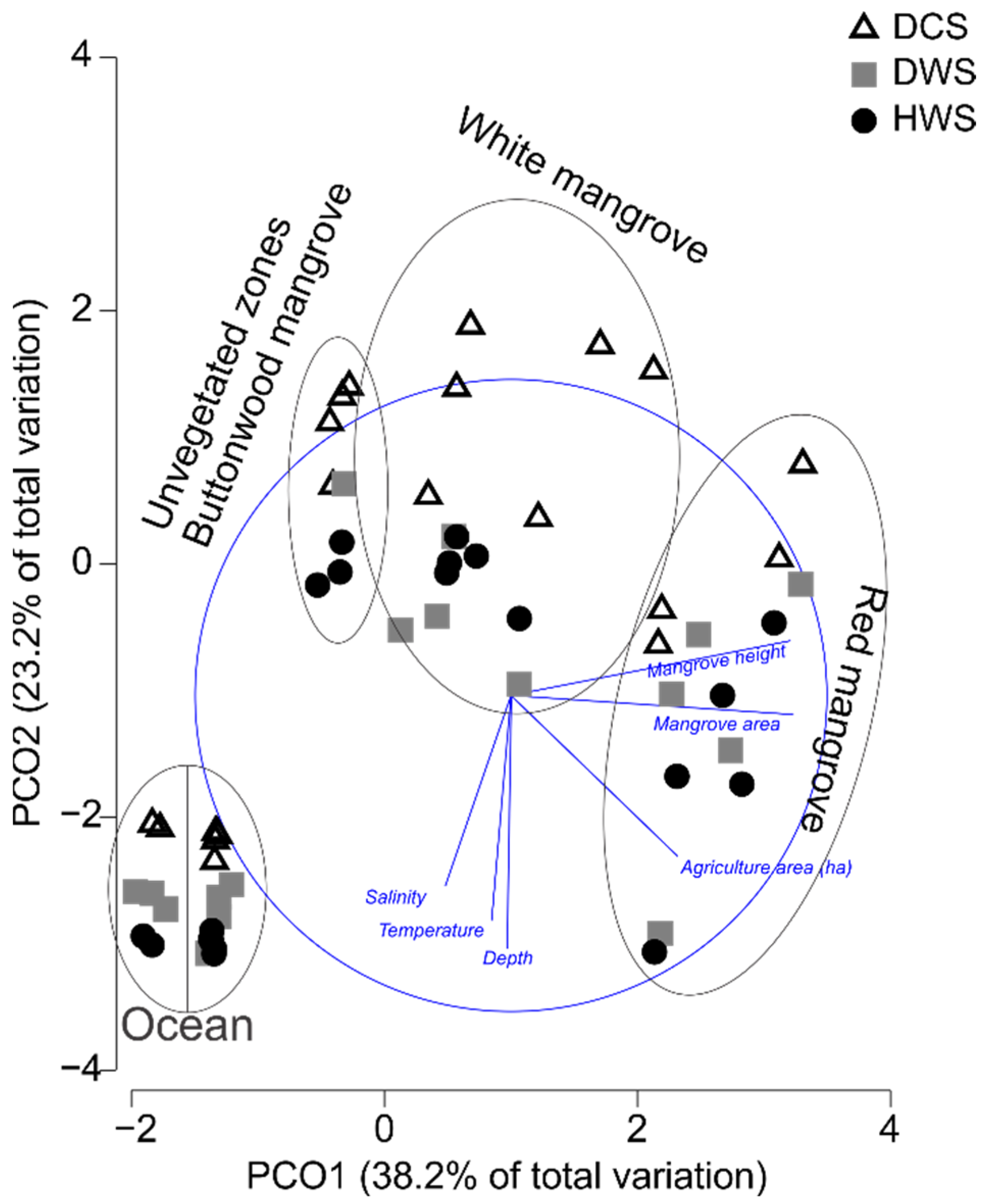
3.1. Environmental Data and Habitat Characteristics

There were marked seasonal differences in water temperature and salinity in both estuarine systems, which followed the established climatic seasons (DCS, DWS, and RWS). The mean water temperature fluctuated from 19.5 °C ± 1.96 (DCS) to 37.1 °C ± 1.37 (RWS), and it changed significantly according to the latter (RWS: F_{(1, 10887)} = 262.59, p < 0.05), which coincides with the summer and early autumn. The salinity showed high variation depending on the zone and season, as it was significantly lower during the rainy season (RWS: F_{(1, 10887)} = 20.534, p < 0.05) at the Huizache lagoon (1.0 ± 0.9 ppt), compared to the dry season at the same estuarine system (35.3 ± 0.6 ppt). In both seasons, the mean salinity was similar in the mouth of the lagoon and the coastal areas. The depth also showed high variations depending on the habitat, where the lagoons and the tidal mangrove creeks were the shallowest habitats (mean depth: 1.07 ± 0.25 m), followed by the river (1.3 ± 0.66 m), the inner tidal channel (3.01 ± 1.7 m), the main tidal channel (5.66 ± 2.6 m), and the oceanic habitats (9.76 ± 4.1 m) that were the deepest habitats of the study area.

A statistically significant correlation was not found among environmental variables after normalization (Pearson’s correlation coefficient = 3.94, p > 0.05). PERMANOVA revealed statistically significant differences between the estuarine system (pseudo-F_1,56 = 6.45, p = 0.001), the climatic season (pseudo-F_2,56 = 5.09, p = 0.001), the habitat (pseudo-F_7,56 = 10.24, p = 0.001), and the zone (pseudo-F_4,56 = 12.6, p = 0.001). In terms of climatic season, differences were found between the warm seasons (DWS and RWS) and the cold one (DCS), but no differences were found between both warm seasons (Supplementary Material Table S1).

For the habitat, the analysis showed well-differentiated groups: the oceanic habitat, Huizache, and Caimanero lagoons, Agua Grande lagoon together with the inner tidal channel, the mangrove creek, and the main tidal channel (Supplementary Material Table S2). In terms of zones, all were different from each other except for unvegetated zones and those inhabited by buttonwood mangroves (Supplementary Material Table S3). The differences between estuarine systems and habitats seemed to be determined by the zones since Teacapan only has red mangroves and ocean zones, while Huizache-Caimanero has white and buttonwood mangroves, unvegetated zones, and the ocean. Although previous studies reported the presence of scattered shrubs (<1 m) of black mangrove (Avicennia germinans) at the basin of the Huizache-Caimanero lagoon [55], the location of this mangrove community is inland without a direct connection with the main body of water. The observed differences were related to environmental variables shown as vectors in the PCoA graph (Figure 2), where clear-cut groups were formed according to zones. The horizontal axis explains most of the variation (38.2%), which is related to mangrove height and cover, which was higher in the red mangrove forest of Teacapan compared to the Huizache-Caimanero system. The vertical axis explains 23.2% of the variation, which is related to depth, temperature, and salinity, which was higher in the ocean of both systems, and in Teacapans’ main tidal channel (where the inlet connects the system with the sea). The extension of the agricultural land was related to both axes and also relevant in Teacapan, where the extension of this zone was higher than the Huizache-Caimanero system.

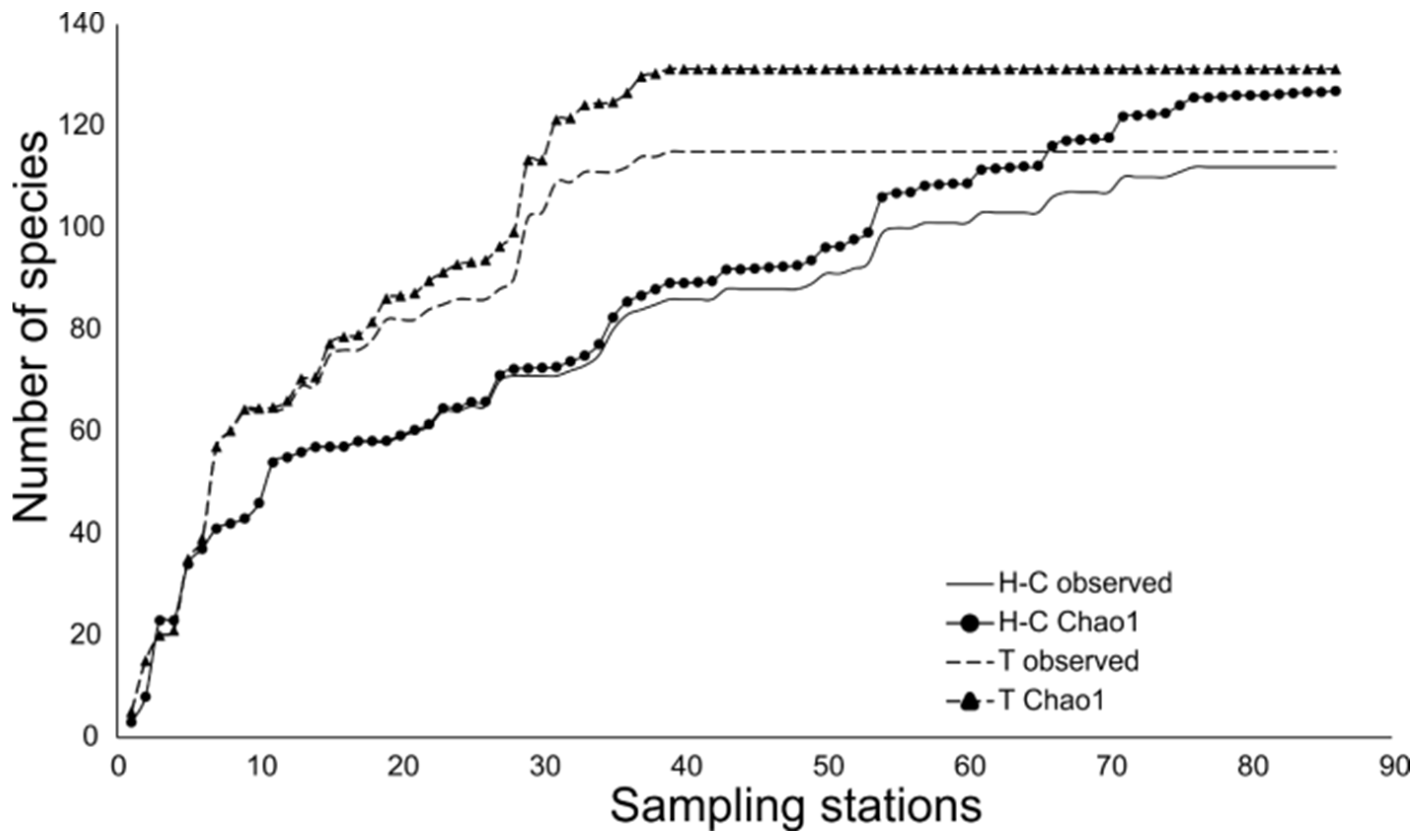
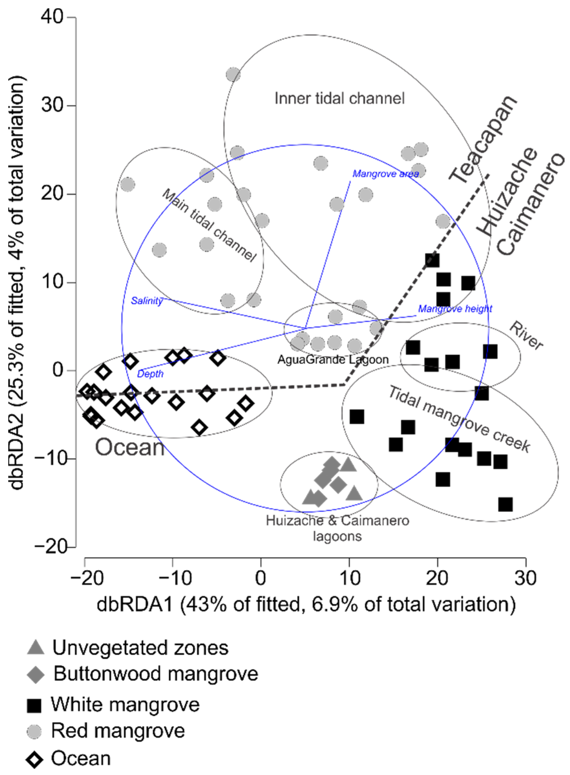
3.2. Fish Assemblages

The sample-based rarefactions using Chao 1 model showed that the sampling effort was representative for both estuarine systems (Figure 3), with 88.23% of the potential species richness recorded in Huizache-Caimanero, and 87.68% in Teacapan.

A total of 12,008 fish individuals were collected pertaining to 143 species (Huizache-Caimanero: 112 species, Teacapan: 115 species recorded), being the most important species in terms of biomass the striped herring Lile stolifera (25.7%), followed by the Congo sea catfish Cathorops fuerthii (7.1%), and the mullet Mugil curema (6.4%). Huizache-Caimanero system was characterized by high biomass of small pelagics (L. stolifera 39.6%, Anchoa walkeri 5.5%), mullets (Mugil curema 7.4%, M. cephalus 5.2%), and the Congo sea catfish (10.1%). In contrast, the Teacapan system did not show any species with such dominance, but two Myliobatiformes accounted for 16% of the total biomass (Rhinoptera steindachneri 10.7%, Aetobatus narinari 5.3%), followed by the tete sea catfish Ariopsis seemanni (10.7%), and the milkfish Chanos chanos (6.15%). The rest of the species represented less than 6% of the total biomass (

Table 1. Abundance and biomass of the fish species analyzed in this study. a = abundance, b = biomass, H = Huizache-Caimanero, T = Teacapan, To = total of the two systems combined, TP = trophic position [56,57].

Family	Species	aH	aT	aTo	bH	bT	bTo	TP
Sphyrnidae	Sphyrna lewini	8	7	15	23.2	25.9	49.1	3.9
Narcinidae	Narcine vermiculata	0	5	5	0	0	0	4.4
Rhinobatidae	Pseudobatos glaucostigma	0	1	1	0	0	0	4
	Pseudobatos leucorhynchus	1	0	1	3.1	0	3.1	3.6
Urotrygonidae	Urobatis halleri	0	1	1	0	0	0	4.6
	Urotrygon chilensis	2	27	29	0	0	0	3.6
	Urotrygon munda	19	0	19	0.1	0	0.1	4.5
	Urotrygon nana	0	4	4	0	0	0	3.6
Mobulidae	Mobula japanica	1	0	1	26.9	0	26.9	3.4
Myliobatidae	Aetobatus narinari	0	2	2	0	134.1	134.1	3.02
	Rhinoptera steindachneri	2	7	9	0.3	272.5	272.8	3.6
Gymnuridae	Gymnura marmorata	0	2	2	0	0	0	4.2
Elopidae	Elops affinis	168	145	313	163.5	75.7	239.2	1.9
Albulidae	Albula nemoptera	1	7	8	0.5	2	2.5	3.9
	Albula vulpes	1	70	71	1.3	94.9	96.2	2
Ophichthidae	Ophichthus zophochir	1	0	1	0.4	0	0.4	3.8
	Myrichthys aspetocheiros	0	1	1	0	0.2	0.2	3.5
Congridae	Ariosoma gilberti	0	1	1	0	0	0	4.4
Pristigasteridae	Opisthopterus dovii	1	0	1	0	0	0	4.2
	Pliosteostoma lutipinnis	133	24	157	11.9	0.3	12.2	3.6
Engraulidae	Anchovia macrolepidota	41	19	60	3.3	1.3	4.6	3.5
	Anchoa lucida	2	1	3	0.1	0	0.1	3.5
	Anchoa mundeola	0	2	2	0	0	0	2
	Anchoa nasus	1	0	1	0.1	0	0.1	3.5
	Anchoa walkeri	464	5	469	255.6	0.1	255.7	3.5
	Cetengraulis mysticetus	21	184	205	0.2	36.5	36.7	3.2
Clupeidae	Dorosoma smithi	0	16	16	0	4	4	3.4
	Lile stolifera	2591	10	2601	1852.8	0	1852.8	1.8
	Opisthonema libertate	15	214	229	7.1	96.5	103.6	2.5
	Opisthonema medirastre	0	2	2	0	0.7	0.7	3.3
Chanidae	Chanos chanos	194	81	275	141.1	155.8	296.9	2
Ariidae	Ariopsis guatemalensis	34	25	59	24.2	53.3	77.5	3.6
	Ariopsis seemanni	34	232	266	41.1	271.3	312.4	3.6
	Bagre panamensis	56	42	98	51.2	79.8	131	4.4
	Bagre pinnimaculatus	5	3	8	3.4	1.8	5.2	4.2
	Cathorops fuerthii	158	84	242	476	39.5	515.5	3.6
	Occidentarius platypogon	46	28	74	84.6	95.8	180.4	4.1
Synodontidae	Synodus scituliceps	0	13	13	0	11.8	11.8	3.6
Fundulidae	Fundulus xenicus	27	0	27	0	0	0	3.2
Mugilidae	Mugil cephalus	331	266	597	242.8	127.9	370.7	3.6
	Mugil curema	432	261	693	348.3	110.6	458.9	2
Hemiramphidae	Hyporhamphus unifasciatus	2	0	2	2.3	0	2.3	3.8
Belonidae	Strongylura exilis	3	0	3	39.9	0	39.9	4.5
	Tylosurus crocodilus	0	1	1	0	5.2	5.2	4.4
Triglidae	Prionotus ruscarius	0	4	4	0	0.6	0.6	3.4
Cichlidae	Oreochromis mossambicus	1	0	1	0.9	0	0.9	1.8
	Oreochromis sp.	437	44	481	162.8	22.7	185.5	1.8
Centropomidae	Centropomus armatus	1	10	11	0.4	1.9	2.3	4.6
	Centropomus medius	3	10	13	1.9	0.1	2	3.2
	Centropomus nigrescens	3	1	4	2.6	0	2.6	3.2
	Centropomus robalito	143	67	210	62.7	6.2	68.9	3.5
	Centropomus viridis	4	17	21	3.8	0.4	4.2	3.8
Serranidae	Epinephelus labriformis	2	0	2	0.4	0	0.4	4
Nematistidae	Nematistius pectoralis	1	48	49	0.3	96.4	96.7	4
Carangidae	Alectis ciliaris	0	1	1	0	0.7	0.7	3.8
	Carangoides otrynter	0	2	2	0	0.7	0.7	4.4
	Caranx caballus	25	45	70	14.9	31.6	46.5	4
	Caranx caninus	169	602	771	66.5	31.7	98.2	3.5
	Caranx vinctus	1	3	4	0.6	2.1	2.7	4
	Chloroscombrus orqueta	177	103	280	39.4	27.3	66.7	3.9
	Hemicaranx leucurus	4	15	19	2	5.5	7.5	4.4
	Hemicaranx zelotes	0	6	6	0	3.4	3.4	4.1
	Oligoplites altus	23	67	90	8.2	69.9	78.1	3.3
	Oligoplites refulgens	5	3	8	1.2	1.5	2.7	4.3
	Oligoplites saurus	5	2	7	4.1	0.5	4.6	3.4
	Selar crumenophthalmus	7	1	8	2.2	0.6	2.8	4.1
	Selene brevoortii	1	9	10	0.1	2.4	2.5	3.6
	Selene orstedii	0	1	1	0	0.3	0.3	3
	Selene peruviana	21	54	75	0.9	9.7	10.6	3.6
	Trachinotus kennedyi	1	3	4	0.5	1.4	1.9	3
	Trachinotus paitensis	2	36	38	2.1	39.6	41.7	2.8
	Trachinotus rhodopus	0	5	5	0	7.8	7.8	4
Lutjanidae	Hoplopagrus guentherii	0	1	1	0	1.2	1.2	3.8
	Lutjanus argentiventris	20	17	37	1.9	13.9	15.8	3.7
	Lutjanus guttatus	0	11	11	0	0	0	3.8
	Lutjanus novemfasciatus	5	3	8	2.4	0.1	2.5	3.5
Gerreidae	Deckertichthys aureolus	3	1	4	0.9	0.2	1.1	3.6
	Diapterus peruvianus	151	503	654	26.9	87.9	114.8	2.2
	Eucinostomus argenteus	14	7	21	9.9	0	9.9	3.6
	Eucinostomus currani	23	97	120	3.7	51.2	54.9	3.6
	Eucinostomus entomelas	53	24	77	17.5	3.5	21	3.5
	Eucinostomus gracilis	0	13	13	0	0.1	0.1	3.8
	Eugerres axillaris	40	42	82	9.7	7.2	16.9	1.7
	Gerres cinereus	22	53	75	6.3	12.6	18.9	3.8
Haemulidae	Conodon serrifer	16	0	16	5.6	0	5.6	3.8
	Pomadasys branickii	2	0	2	0.8	0	0.8	3.9
	Rhencus macracanthus	74	95	169	32.9	101.4	134.3	3.2
	Rhencus panamensis	28	42	70	12.3	32.6	44.9	3.8
	Brachygenys californiensis	0	1	1	0	0	0	3.5
	Orthopristis chalceus	1	1	2	1	0	1	3.6
	Haemulopsis axillaris	31	0	31	17.4	0	17.4	3.8
	Haemulopsis leuciscus	7	5	12	4.8	4.2	9	3.8
	Haemulopsis nitidus	12	49	61	5.2	7.4	12.6	3.7
Polynemidae	Polydactylus approximans	18	11	29	43.2	11.5	54.7	4.1
	Polydactylus opercularis	1	0	1	0.3	0	0.3	3.3
Sciaenidae	Bairdiella icistia	2	0	2	0.8	0	0.8	3.9
	Isopisthus remifer	7	70	77	1.7	0.2	1.9	4.4
	Cynoscion othonopterus	1	0	1	0.9	0	0.9	3.9
	Cynoscion reticulatus	30	11	41	8.7	1.6	10.3	4.7
	Cynoscion squamipinnis	11	0	11	6.9	0	6.9	3.9
	Cynoscion stolzmanni	24	3	27	8.3	3.1	11.4	4.5
	Cynoscion xanthulus	192	8	200	138.8	5.1	143.9	4.3
	Larimus acclivis	2	0	2	0	0	0	4
	Larimus effulgens	132	13	145	9.3	3.3	12.6	3.7
	Stellifer fuerthii	146	79	225	1.2	0.8	2	3.7
	Stellifer illecebrosus	86	0	86	1.5	0	1.5	4.1
	Stellifer sp.	0	3	3	0	0	0
	Umbrina xanti	3	1	4	2.1	3.5	5.6	3.6
	Menticirrhus elongatus	5	1	6	3.3	0	3.3	3.5
	Menticirrhus nasus	4	5	9	2	15.1	17.1	3.6
	Micropogonias altipinnis	27	0	27	10.4	0	10.4	3.7
	Micropogonias ectenes	9	5	14	5.7	2.1	7.8	3.8
	Micropogonias megalops	0	6	6	0	0	0	3.4
	Paralonchurus goodei	40	12	52	1.5	0	1.5	3.9
Mullidae	Pseudupeneus grandisquamis	0	5	5	0	0	0	3.8
Chaetodontidae	Chaetodon humeralis	0	1	1	0	0.4	0.4	2.7
Pomacentridae	Abudefduf troschelii	0	1	1	0	0	0	3.9
Labridae	Bodianus diplotaenia	2	0	2	1.3	0	1.3	3.4
Eleotridae	Gobiomorus maculatus	33	12	45	4.2	0.9	5.1	1.7
	Dormitator latifrons	112	120	232	34.2	1.7	35.9	1.9
	Eleotris picta	1	0	1	1.6	0	1.6	3.9
Gobiidae	Microgobius sp.	1	1	2	0	0	0
	Gobionellus microdon	16	3	19	0.9	0.1	1	1.8
Ephippidae	Chaetodipterus zonatus	4	23	27	2	6	8	2.5
Sphyraenidae	Sphyraena ensis	1	0	1	3.7	0	3.7	3.9
Trichiuridae	Trichiurus lepturus	2	0	2	0	0	0	3.9
Scombridae	Scomber japonicus	4	3	7	4.7	2.1	6.8	3.4
	Scomberomorus sierra	18	1	19	19.3	5.5	24.8	3.8
	Katsuwonus pelamis	0	3	3	0	52.7	52.7	4.3
Stromaetidae	Peprilus medius	20	10	30	7.2	4.6	11.8	3.9
	Peprilus snyderi	10	24	34	3.5	22.3	25.8	4.3
Paralichthydae	Paralichthys woolmani	1	0	1	3.4	0	3.4	4.5
	Syacium ovale	1	6	7	0	0	0	3.5
	Cyclopsetta panamensis	5	7	12	0	2.8	2.8	3.7
	Cyclopsetta querna	8	5	13	1.5	3.8	5.3	3.7
	Citharichthys gilberti	2	0	2	0.1	0	0.1	4.1
	Etropus crossotus	6	0	6	0.2	0	0.2	4
Achiridae	Achirus mazatlanus	70	134	204	6	0.3	6.3	3.7
	Trinectes fonsecensis	4	3	7	0	0	0	3.8
Cynoglossidae	Symphurus elongatus	93	4	97	0.1	0	0.1	4.1
Ballistidae	Balistes polylepis	1	3	4	0	0.1	0.1	3.4
Tetraodontidae	Sphoeroides annulatus	0	2	2	0	0.1	0.1	3.8
	Sphoeroides lobatus	0	4	4	0	0	0	4

).

In terms of abundance in both estuarine systems, the striped herring (21.7%), the mullets (11.7%), and the Pacific crevalle jack (Caranx caninus) presented a high proportion (6.42%). Huizache-Caimanero was also characterized by a high number of small pelagics (L. stolifera 34.6%, A. walkeri 6.2%) and mullets (Mugil curema 5.8%, M. cephalus 4.4%), but the invasive species of tilapia (Oreochromis spp.) also presented high abundance (5.8%). In Teacapan, the two most important species in terms of the number of individuals were the Pacific crevalle jack (C. caninus, 13.3%) and the mojarra (Diapterus peruvianus, 11.1%; Table 1).

Species richness between zones presented differences, with the highest values in the ocean zone of Teacapan (90 species) and Huizache-Caimanero (72 species), followed by the red mangrove forest (70 species), the white mangrove forest (57 species), the buttonwood mangrove forest (51 species), and the unvegetated zone with 28 fish species. The PERMANOVA results showed significant differences among estuarine systems (pseudo-F_1,56 = 2.483, p = 0.003), habitat (pseudo-F_7,56 = 2.283, p = 0.001), and zones (pseudo-F_4,56 = 2.8, p = 0.001), but no differences were found among climatic seasons (pseudo-F_2,56 = 1.206, p = 0.177). The pairwise comparisons showed that most of the habitat presented different fish assemblages, except for Caimanero and Huizache lagoons (t = 1.12, p = 0.026), and these with the tidal mangrove creek, the inner tidal channels and the river at this estuarine system. In the Teacapan system, the inner tidal channel, the tidal mangrove creek, and the Agua Grande lagoon did not present significant differences (Supplementary Material Table S4). In terms of zones, the pairwise comparisons between them showed that only the unvegetated zone and buttonwood mangrove forest were not statistically different (t = 0.894, p = 0.603; Supplementary Material Table S5).

The DistLM marginal test (

Table 2. Marginal test of the distance-based linear model (DISTLM) showing the relationships of the different environmental factors with the fish assemblages. * indicates statistically significant results.

Variable	SS (Trace)	Pseudo-F	p	Prop.
Temperature	3815.5	1.07	0.34	0.02
Salinity *	10,101.0	2.92	0.00	0.05
Mangrove height *	10,311.0	2.98	0.00	0.05
Mangrove area *	7993.2	2.28	0.00	0.04
Agriculture area	5557.6	1.57	0.14	0.03
Depth *	12,166.0	5.03	0.00	0.16

) indicated that salinity, the mangrove height, the mangrove area, and depth were significant predictors of fish biomass. This information was used to create a dbRDA plot (Figure 4), in which the first two axes explained 68.24% of the variability in the fitted model, and where the horizontal axis showed a gradient across zones, with high to low salinity and depth from left to right, and high (white mangrove) to low (red mangrove) mangrove height from right to left. Higher salinities and depths were found in the oceanic habitat of both estuarine systems and the main tidal channel of Teacapan, while the inner parts of the estuarine systems were shallow and presented low salinity due to the influence of freshwater inputs.

In the vertical axis, a gradient of high to low mangrove cover was observed, with higher values in Teacapan (due to large extensions of red mangrove forests), compared with Huizache-Caimanero, which presented small to medium patches of white mangrove. According to the dbRDA, which includes the information on fish assemblages’ composition (Figure 4), the sampled stations of Teacapan were grouped in the top left, while the ones of Huizache-Caimanero were grouped in the bottom right. In this analysis, four habitat types were identified, which are similar to the results from the PERMANOVA: oceanic zone, buttonwood mangrove forests/unvegetated zones, white mangrove forests, and red mangrove forests. Evident groups according to habitats were not observed, although the fish assemblages from the same habitat grouped close to each other.

The fish species that contribute to the Huizache-Caimanero aggrupation were mainly the mullets (M. curema and M. cephalus), the machete (Elops affinis), the tilapia (Oreochromis spp.), and the Pacific fat sleeper (Dormitator latifrons), while in Teacapan, the main contributing species were the Pacific cownose ray (R. steindachneri), grunts (Rhencus macracanthu and Haemulopsis leuciscus), and catfishes (Ariopsis seemanni and Cathorops fuerthii).

For habitats, the fish species contributing prominently to the oceanic assemblage were the common hammerhead shark (Sphyrna lewini), the Pacific cownose ray, the jack (C. caninus), scombrids (Scomber japonicus and Katsuwonus pelamis), and demersal species such as catfishes (Bagre panamensis and Occidentarius platypogon) and croakers (Micropogonias altipinnis, Cynoscion squamipinnis, C. stolzmanni, and Umbrina xanti). For the red mangrove zone, a suite of species from different environments was found, including marine organisms present in the main tidal channel such as golden cownose ray (R. steindachneri), marine and estuarine species such as grunts (R. macracanthus, Oligoplites spp., Pomadasys spp., Haemulopsis spp.), catfishes, and the roosterfish (Nematistius pectoralis). Typical estuarine species such as the milkfish (C. chanos) and snooks (Centropomus spp.) were present in this zone. For the white mangrove zone, which includes all the channels in the Huizache-Caimanero system, the most representative species were two small pelagics (striped herring L. stolifera and persistent anchovy A. walkeri), the machete (E. affinis), and mullets (M. curema and M. cephalus), which were also the most abundant species in this estuarine system. For the buttonwood mangrove forests/unvegetated zone, the tilapia (Oreochromis spp.) and the Pacific fat sleeper (D. latifrons), which are usually freshwater species, were the ones characterizing this zone.

Although the three measures of alpha diversity (⁰D, ¹D, and ²D) tended to decrease from the oceanic zone towards the inner parts of the estuaries (Figure 5), only the oceanic zone showed statistical differences with higher values than the other zones according to the GAMs (t⁰_D = 2.07, p < 0.05; t¹_D = 2.768, p < 0.05; t²_D = 2.881, p < 0.05). For all the other cases, GAMs showed values of t < 1.9, p > 0.05.

For beta diversity, the nestedness component (species richness differences) did not show significant differences between zones (tβ_sne < 1.6, p > 0.2), while the spatial turnover (species replacement) was different, due to the higher values in the ocean (tβ_stu > 28.94, p < 0.01) compared to the rest of the zones that did not show significant differences among them at the pairwise analyses (t < 0.98, p > 0.32).

4. Discussion

On a global scale, comparisons of wetland equivalence across regions have begun to appear in the literature [58,59], but caution is advised, especially when they do not account for biases caused by the sampling of different zones and habitats, or the use of different sampling methodologies and effort. This study is the first comparison of the fish assemblages in tropical wetland ecosystems from the same geographical region that accounts for different habitats and standardizes the sampling methodologies.

4.1. Environmental Data and Habitat Characteristics

The seasonal variation in temperature and salinity reported in this study is similar to findings for other tropical regions [7] and the variability previously registered for these systems [31]. In addition, differences were also observed between estuarine systems, with Teacapan being classified as a tide-dominated estuary while Huizache-Caimanero could be considered as an intermittent estuary. The measure of physical, biological, and other environmental variables also allowed identifying zones within the studied systems. The first zone corresponds to the estuarine habitats in Teacapan inhabited by the good conditions of the red mangrove forests are reflected by their high height and cover, despite the presence of agricultural lands in contiguous areas. In contrast, the Huizache-Caimanero system showed two zones corresponding to white mangrove and the buttonwood mangrove/unvegetated zones, but with a deteriorated condition, and therefore less height and covered area. This condition has been previously reported [31] and was attributable to large human settlements nearby. Finally, another zone was identified in the oceanic area for both estuarine systems.

Regarding physicochemical and environmental parameters, salinity, temperature, and depth were higher in the oceanic zone, with an observed gradient from the main tidal channel connected to the sea, toward the inner channels of Teacapan and Agua Grande lagoons where the depth decreases considerably and the effect of the river drainage increase, reducing the salinity and temperature. For Huizache-Caimanero, an abrupt difference was observed due to the limited connection to the sea associated with shallow depths and high sedimentation. Therefore, the inner parts were more influenced by the drainage of the rivers Presidio and Baluarte, which decreased the salinity and temperature. A change associated with the season was observed in all zones, DCS showed lower temperatures and higher salinities, DWS higher temperature and salinity, and the RWS with lower salinities and higher temperatures. Nonetheless, this factor was not as important as other variables for defining zones and habitats within the systems.

4.2. Fish Assemblages

The most comprehensive study of the ichthyofauna in the southern Sinaloa shelf, which included both systems studied in the present work, registered 600 fish species from the coastal area up to the isobath of 110 m with an approximate study area of 6400 km² with a perimeter of ~700 km, using a large suite of fishing gears (trawl nets, gill nets, seine nets, hook and line, spearguns, and rotenone) and boats (from skiffs to research vessels; [60]). In contrast, the present study registered fewer species (143 species), which could be associated with a less covered area of ~200 km² (150 km² at Huizache-Caimanero and 50 km² at Teacapan), shallower sampling depths (~20 m in the oceanic area adjacent to the systems), and fewer fishing techniques employed (gill nets, seine nets, and cast nets fitted in skiffs).

The total species richness registered in the present work represents 23.8% of the total reported in the area, where the richness of Teacapan represents 19.2%, and the one in Huizache-Caimanero represents 18.7%; therefore, in terms of richness per km², the value in Teacapan is higher. The number of species found in this work is higher than those previously reported in the same systems [31], which reported values between 44 and 61 species for Huizache-Caimanero, and 51 to 76 species for Teacapan [34,35,37,59].

The richness reported in this paper is higher compared to other estuarine ecosystems in the Tropical Mexican Pacific, such as a coastal lagoon of Oaxaca [61] or two estuarine lagoon systems in southern Chiapas [62]. These results are consistent with the range of species richness values for the 12 coastal lagoons along the Mexican Pacific coast, which is between 3 and 73 species with an average of 30 species [63].

According to the rarefaction models, the species found in the present study are close to the estimated number of species per estuarine system. Therefore, the differences with previous studies seem to be related to the sampling effort, the area covered, and the variety of fishing gears utilized, besides other intrinsic characteristics of the estuarine systems that might affect the richness, such as the presence and cover of mangrove forests, and human activities (e.g., fishing, agricultural lands [64,65,66]).

In species composition terms, Huizache-Caimanero is habited mostly by small pelagics, as these species had already been reported as the main component of fish larvae in this system [67] and represented the higher biomass in the present study. Considering that this system has low salinity throughout the year due to its characteristic as an intermittent estuary with a strong influence of two rivers, the expectation was that species with a stronger association to brackish and freshwater were dominant. In the Teacapan case, the influence of a large inlet and a permanent connection to the sea influences the species composition, as two batoids were the most important species in terms of biomass, but the typical estuarine conditions of this system seem to favor the presence of species as catfish.

According to the PERMANOVA and the DistLM analyses, fish assemblages seemed to be characterized by the a priori defined zones and then by the habitats. The variables that showed an effect on the structure and composition of the fish assemblages were salinity, depth, agriculture area, and mangrove height and area, which explained 43% of the fitted variation. Salinity and depth were significant predictors in the oceanic zone and gradually decreased toward the inner parts of the Teacapan system, in which fish assemblages also was influenced by the red mangrove height and covered area. In contrast, for Huizache-Caimanero, an abrupt change in species composition from the ocean to the inner zones was observed, probably due to the seasonal ephemeral inlet that limits the seas’ influence on this system during the dry season. However, a gradual change in fish species composition was observed in the inner zones from the white mangrove forests toward unvegetated zones and buttonwood mangrove forests predicted by the mangrove height.

The vertical axis from the dbRDA plot explained 25.3% of the fitted variation, indicating that another important predictor was the extension of the mangrove forests, which was more prominent in the red mangroves of Teacapan and some limited areas of the white mangroves of Huizache-Caimanero. The height of the mangrove trees and the overall extent of the forest can be considered as a proxy for determining the ecological status of the ecosystem in semiarid regions [31]. The mangrove areas where the forest has tall trees with large basal areas and low density of stems are indicative of sites with pristine conditions by estuarine circulation (as the red mangrove forests of Teacapan), or with a strong and persistent influence of freshwater inputs (as the white mangrove forests of Huizache-Caimanero). In the case of the buttonwood mangrove forests and unvegetated zones, these zones result from the combination of intermittent freshwater inputs and shallow areas with a high rate of sedimentation.

According to the SIMPER, the oceanic zone in both systems was predominantly inhabited by marine species such as pelagic elasmobranchs, scombrids, and jacks, as well as by demersal species that enter the estuarine systems as croakers (Sciaenidae) and catfish, among other species. The red mangrove zone, which included all the inner habitats at Teacapan, was characterized by marine species such as pelagic batoids and estuarine species like milkfish and snooks (Centropomus spp.), as well as species that use these zones to complete parts of their life cycle such as roosterfish, drum, and catfish. Specifically, the catfish was already characterized as key species for this system [31] because it requires the typical estuarine variation in salinity to complete its life cycle [68]. Thus, the presence of this species in the area might be indicative of the importance of seasonal fluctuations to the growth and colonization of fish in red mangroves habitats. Similarly, in the white mangrove forests, the dominance of tilapia, herrings, and anchovies that usually inhabit freshwater and estuarine ecosystems [69] might be an indicator of the effect of the salinity and the hydrological regime on the composition of fish assemblages.

The buttonwood mangrove/unvegetated zone, which included the lagoons of Huizache-Caimanero, was a shallow area (~1 m depth) that presented mud and standing water with low salinity. In this area, the characteristic species were tilapias and sleepers, which inhabit brackish and freshwater areas with muddy and sandy sediments [69]. Altogether, these results indicate that fish assemblages respond to the surrounding environment, which also influences the zone, defined by the vegetation. Typical estuarine systems with hydrological regimes that favor the presence of red mangroves as Teacapan are inhabited by a large suite of fish, including marine and estuarine species that require typical estuarine systems to complete their life cycles.

In contrast, zones with predominantly freshwater and brackish conditions as the channels in the Huizache-Caimanero system favor the presence of white mangroves that will be inhabited by estuarine species that can tolerate these conditions. Finally, shallow, muddy, standing waters with low salinity such as Huizache-Caimanero lagoons are not adequate for mangrove forests to thrive; thus, they are inhabited by other species that prefer those conditions generated by the lack of connection with the Pacific Ocean that restricts the influence of saltwater, especially during the dry season when the ephemeral inlet of the Presidio River mouth remains closed by a sand barrier. At the beginning of the rainy season, the freshwater flow throughout the Presidio River increases considerably, even though the mouth remains closed by the sand barrier that starts breaking only if the amount of freshwater is sufficient, thus opening the lagoon to the ocean.

While there are no published works regarding this physical process at the Presidio River [70], a study at a similar ephemeral river (Quelite) with mangrove ecosystems located 50 km north of Huizache-Caimanero showed that the overall process of opening the sand barrier generally takes a few days, and the result consists of a massive plume of freshwater input into the ocean [71]. Thus, opening the sand barrier at the Huizache-Caimanero lagoon could result in an increase in the amount of freshwater from the Presidio River to the oceanic zone, causing an overall decrease in salt concentration and temperature within the coastal system and changes in the associated fish assemblages.

The complexity of the mangrove habitat, red in Teacapan and white in the Huizache-Caimanero estuarine systems, attracts many fish species that utilize the mangrove as breeding and nursery areas for juveniles. For example, the red mangrove develops a complex network of aerial roots towards the main water body that protects juvenile fish and other organisms from large predators [11,72]. In the case of the white mangrove, it does not have aerial roots, so its function as a protected area for juvenile fish could be reduced compared to the red mangrove. However, the white mangrove tends to thrive in coastal systems with low salinity, which limits the access of oceanic predators.

Related to nutrient availability, mangrove-dominated habitats are different from other coastal ecosystems and therefore favor the presence of fishery resources at the nursery and breeding stages [23,32]. Previous studies have found that species composition, biomass, and diversity of estuarine fish have strong relationships with the different environmental factors, especially temperature and salinity [3]. Our results revealed the importance of salinity in defining fish assemblages’ composition, as this factor could act as a physiological barrier due to osmoregulatory stress or reduced foraging efficiency, which is often reflected by low fish species richness, biomass, and mixed fish composition of marine, estuarine, and freshwater species [14,18,27,73,74].

Factors contributing to these patterns seemed to be a combination of changes in habitat structure (especially the presence or absence of mangrove trees), water conditions, and substratum characteristics. One of the reasons for the increased diversity of fish in the oceanic zone could be associated with high habitat complexity that allows the presence of a wide variety of species with distinct requirements for reproduction, refugee, and food [11,12]. In addition, red mangrove areas of Teacapan also presented high species richness, which might be associated with the nutrient supply from the nearby mangrove areas that are consumed directly (e.g., detritus) or indirectly (through the structure features attracting prey) by different fish species [75].

Studies have shown that losses of mangrove habitats had negative effects on the fish biomass and diversity [18,76]. However, during the last decade, deforestation of mangrove forests has been extensive throughout the world [77,78,79]. Describing differences in fish assemblages’ composition at each habitat and the relation with environmental variables is essential to understand fish fauna dynamics at these “critical habitats” and to propose local management strategies for each estuarine system [80] based on the life histories of its species and the different hydrological factors reported at the Teacapan and Huizache-Caimanero lagoons in the present study.

References

1. Kandasamy, K.; Bingham, B. Biology of Mangroves and Mangrove Ecosystems. Adv. Mar. Biol. 2001, 40, 81–251. [Google Scholar] [CrossRef]
2. Crona, B.I.; Rönnbäck, P. Use of Replanted Mangroves as Nursery Grounds by Shrimp Communities in Gazi Bay, Kenya. Estuar. Coast. Shelf Sci. 2005, 65, 535–544. [Google Scholar] [CrossRef]
3. Chowdhury, M.S.N.; Hossain, M.S.; Das, N.G.; Barua, P. Environmental Variables and Fisheries Diversity of the Naaf River Estuary, Bangladesh. J. Coast. Conserv. 2011, 15, 163–180. [Google Scholar] [CrossRef]
4. Hossain, M.S.; Gopal Das, N.; Sarker, S.; Rahaman, M.Z. Fish Diversity and Habitat Relationship with Environmental Variables at Meghna River Estuary, Bangladesh. Egypt. J. Aquat. Res. 2012, 38, 213–226. [Google Scholar] [CrossRef] [Green Version]
5. Larson, M. Coastal Lagoons. In Encyclopedia of Lakes and Reservoirs; Bengtsson, L., Herschy, R.W., Fairbridge, R.W., Eds.; Springer Netherlands: Dordrecht, The Netherlands, 2012; pp. 171–173. ISBN 978-1-4020-4410-6. [Google Scholar]
6. Barletta, M.; Amaral, C.S.; Corrêa, M.F.M.; Guebert, F.; Dantas, D.V.; Lorenzi, L.; Saint-Paul, U. Factors Affecting Seasonal Variations in Demersal Fish Assemblages at an Ecocline in a Tropical-Subtropical Estuary. J. Fish Biol. 2008, 73, 1314–1336. [Google Scholar] [CrossRef]
7. Blaber, S.J.M. Tropical Estuarine Fishes: Ecology, Exploitation and Conservation; John Wiley & Sons: Hoboken, NJ, USA, 2008; ISBN 0470694874. [Google Scholar]
8. Franco, A.; Pérez-Ruzafa, A.; Drouineau, H.; Franzoi, P.; Koutrakis, E.T.; Lepage, M.; Verdiell-Cubedo, D.; Bouchoucha, M.; López-Capel, A.; Riccato, F.; et al. Assessment of Fish Assemblages in Coastal Lagoon Habitats: Effect of Sampling Method. Estuar. Coast. Shelf Sci. 2012, 112, 115–125. [Google Scholar] [CrossRef]
9. Rodríguez-Romero, J.; del Carmen López-González, L.; Galván-Magaña, F.; Sánchez-Gutiérrez, F.; Inohuye, R.; Pérez-Urbiola, J. Seasonal Changes in a Fish Assemblage Associated with Mangroves in a Coastal Lagoon of Baja California Sur, Mexico. Lat. Am. J. Aquat. Res. 2011, 39, 250–260. [Google Scholar] [CrossRef]
10. Franco, A.; Franzoi, P.; Malavasi, S.; Riccato, F.; Torricelli, P.; Mainardi, D. Use of Shallow Water Habitats by Fish Assemblages in a Mediterranean Coastal Lagoon. Estuar. Coast. Shelf Sci. 2006, 66, 67–83. [Google Scholar] [CrossRef]
11. Laegdsgaard, P.; Johnson, C. Why Do Juvenile Fish Utilise Mangrove Habitats? J. Exp. Mar. Biol. Ecol. 2001, 257, 229–253. [Google Scholar] [CrossRef] [Green Version]
12. Verweij, R.; Verrelst, J.; Loth, P.E.; Heitkonig, I.; Brunsting, A.M.H. Grazing Lawns Contribute to the Subsistence of Mesoherbivores on Dystrophic Savannas. Oikos 2006, 114, 108–116. [Google Scholar] [CrossRef]
13. Lugendo, B.; Nagelkerken, I.; Kruitwagen, G.; Van der Velde, G.; Mgaya, Y. Relative Importance of Mangroves as Feeding Habitats for Fishes: A Comparison between Mangrove Habitats with Different Settings. Bull. Mar. Sci. 2007, 80, 497–512. [Google Scholar]
14. Robertson, A.I.; Duke, N.C. Mangrove Fish-Communities in Tropical Queensland, Australia: Spatial and Temporal Patterns in Densities, Biomass and Community Structure. Mar. Biol. 1990, 104, 369–379. [Google Scholar] [CrossRef]
15. Krumme, U.; Saint-Paul, U. Observations of Fish Migration in a Macrotidal Mangrove Channel in Northern Brazil Using a 200 kHz Split-Beam Sonar. Aquat. Living Resour. 2003, 16, 175–184. [Google Scholar] [CrossRef]
16. Matheson, R.; Gilmore, R.G. Mojarras (Pisces: Gerreidae) of the Indian River Lagoon. Bull. Mar. Sci. 1995, 57, 281–285. [Google Scholar]
17. Ikejima, K.; Tongnunui, P.; Medej, T.; Taniuchi, T. Juvenile and Small Fishes in a Mangrove Estuary in Trang Province, Thailand: Seasonal and Habitat Differences. Estuar. Coast. Shelf Sci. 2003, 56, 447–457. [Google Scholar] [CrossRef]
18. Shervette, V.R.; Aguirre, W.E.; Blacio, E.; Cevallos, R.; Gonzalez, M.; Pozo, F.; Gelwick, F. Fish Communities of a Disturbed Mangrove Wetland and an Adjacent Tidal River in Palmar, Ecuador. Estuar. Coast. Shelf Sci. 2007, 72, 115–128. [Google Scholar] [CrossRef]
19. Sheridan, P.; Hays, C. Are Mangroves Nursery Habitat for Transient Fishes and Decapods? Wetlands 2003, 23, 449–458. [Google Scholar] [CrossRef]
20. Mumby, P.J.; Edwards, A.J.; Arias-González, J.E.; Lindeman, K.C.; Blackwell, P.G.; Gall, A.; Gorczynska, M.I.; Harborne, A.R.; Pescod, C.L.; Renken, H.; et al. Mangroves Enhance the Biomass of Coral Reef Fish Communities in the Caribbean. Nature 2004, 427, 533–536. [Google Scholar] [CrossRef] [Green Version]
21. Barletta, M.; Barletta-Bergan, A.; Saint-Paul, U.; Hubold, G. The Role of Salinity in Structuring the Fish Assemblages in a Tropical Estuary. J. Fish Biol. 2005, 66, 45–72. [Google Scholar] [CrossRef]
22. Whitfield, A. Abundance of Larval and 0+juvenile Marine Fishes in Three Southern African Estuaries with Differing Freshwater Inputs. Mar. Ecol. Ser. Mar. Ecol. Prog. Ser. 1994, 105, 257–267. [Google Scholar] [CrossRef]
23. Huxham, M.; Kimani, E.; Augley, J. Mangrove Fish: A Comparison of Community Structure between Forested and Cleared Habitats. Estuar. Coast. Shelf Sci. 2004, 60, 637–647. [Google Scholar] [CrossRef]
24. Blaber, S.; Brewer, D.; Harris, A.N. Distribution, Biomass and Community Structure of Demersal Fishes of the Gulf of Carpentaria, Australia. Mar. Freshw. Res. 1994, 45, 375–396. [Google Scholar] [CrossRef]
25. Nagelkerken, I.; Faunce, C. Colonisation of Artificial Mangrove Shorelinies by Reef Fishes in a Marine Landscape. Estuar. Coast. Shelf Sci. 2007, 75, 417–422. [Google Scholar] [CrossRef]
26. Barletta, M.; Barletta-Bergan, A.; Saint-Paul, U.; Hubold, G. Seasonal Changes in Density, Biomass, and Diversity of Estuarine Fishes in Tidal Mangrove Creeks of the Lower Caeté Estuary (Northern Brazilian Coast, East Amazon). Mar. Ecol. Prog. Ser. 2003, 256, 217–228. [Google Scholar] [CrossRef] [Green Version]
27. Serafy, J.; Faunce, C.; Lorenz, J. (Jerry) Mangrove Shoreline Fishes of Biscayne Bay, Florida. Bull. Mar. Sci. 2003, 72, 161–180. [Google Scholar]
28. Pittman, S.; Mcalpine, C.; Pittman, K. Linking Fish and Prawns to Their Environment: A Hierarchical Landscape Approach. Mar. Ecol. Prog. Ser. 2004, 283, 233–254. [Google Scholar] [CrossRef]
29. Blaber, S. Mangroves and Fishes: Issues of Diversity, Dependence, and Dogma. Bull. Mar. Sci. 2007, 80, 457–472. [Google Scholar]
30. Gullström, M.; Bodin, M.; Nilsson, P.; Öhman, M. Seagrass Structural Complexity and Landscape Configuration as Determinants of Tropical Fish Assemblage Composition. Mar. Ecol. Prog. Ser. 2008, 363, 241–255. [Google Scholar] [CrossRef] [Green Version]
31. Amezcua, F.; Ramirez, M.; Flores-Verdugo, F. Classification and Comparison of Five Estuaries in the Southeast Gulf of California Based on Environmental Variables and Fish Assemblages. Bull. Mar. Sci. 2019, 95, 139–159. [Google Scholar] [CrossRef]
32. Rönnbäck, P.; Troell, M.; Kautsky, N.; Primavera, J.H. Distribution Pattern of Shrimps and Fish AmongAvicenniaandRhizophoraMicrohabitats in the Pagbilao Mangroves, Philippines. Estuar. Coast. Shelf Sci. 1999, 48, 223–234. [Google Scholar] [CrossRef]
33. Attrill, M.; Rundle, S. Ecotone or Ecocline: Ecological Boundaries in Estuaries. Estuar. Coast. Shelf Sci. 2002, 55, 929–936. [Google Scholar] [CrossRef]
34. Rubio-Alvarez, M.; Amezcua-Linares, F.; Yáñez-Arancibia, A. Ecología y Estructura de Las Comunidades de Peces En El Sistema Lagunar Teacapán-Agua Brava, Nayarit, México. An. Inst. Cienc. Mar Limnol. 1986, 13, 185–242. [Google Scholar]
35. Amezcua-Linares, F. Generalidades Ictiológicas Del Sistema Lagunar Costero de Huizache-Caimanero, Sinaloa, México. Anales 1977, 4, 1–26. [Google Scholar]
36. Amezcua-Linares, F.; Álvarez-Rubio, M.; Yáñez-Arancibia, A. Dinámica y Estructura de La Comunidad de Peces En Un Sistema Ecológico de Manglares de La Costa Del Pacífico de México, Nayarit. An. Inst. Cienc. Mar Limnol. 1987, 14, 221–248. [Google Scholar]
37. Flores-Verdugo, F.; González-Farías, F.; Ramírez-Flores, O.; Amezcua-Linares, F.; Yáñez-Arancibia, A.; Alvarez-Rubio, M.; Day, J.W. Mangrove Ecology, Aquatic Primary Productivity, and Fish Community Dynamics in the Teacapán-Agua Brava Lagoon-Estuarine System (Mexican Pacific). Estuaries 1990, 13, 219–230. [Google Scholar] [CrossRef]
38. Fischer, W.; Krupp, F.; Schneider, W.; Sommer, C.; Carpenter, K.; Niem, V. Guía FAO Para la Identificación de Especies Para Los Fines de la Pesca, Pacífico Centro-Oriental; FAO: Rome, Italy, 1995; ISBN 92-5-303408-4. [Google Scholar]
39. Amezcua-Linares, F. Peces Demersales del Pacífico de México; Instituto de Ciencias del Mar y Limnología, Universidad Nacional Autónoma de México: Ciudad de México, México, 2009; ISBN 978-970-764-558-5. [Google Scholar]
40. Anderson, M.J.; Gorley, R.N.; Clarke, K.R. PRIMER+ for PERMANOVA: Guide to Software and Statistical Methods. 214; Primer-e: Plymouth, UK, 2008. [Google Scholar]
41. Anderson, M.J. Permutational Multivariate Analysis of Variance (PERMANOVA). Wiley StatsRef Stat. Ref. Online 2017, 1, 1–15. [Google Scholar] [CrossRef]
42. Carson, H.S.; Ulrich, M.; Lowry, D.; Pacunski, R.E.; Sizemore, R. Status of the California Sea Cucumber (Parastichopus Californicus) and Red Sea Urchin (Mesocentrotus Franciscanus) Commercial Dive Fisheries in the San Juan Islands, Washington State, USA. Fish. Res. 2016, 179, 179–190. [Google Scholar] [CrossRef]
43. Chao, A. Nonparametric Estimation of the Number of Classes in a Population. Scand. J. Stat. 1984, 11, 265–270. [Google Scholar]
44. Magurran, A.E. Measuring Biological Diversity, 1st ed.; Blakwell Publishing: Oxford, UK, 2004; ISBN 0-632-05633-9. [Google Scholar]
45. McArdle, B.H.; Anderson, M.J. Fitting Multivariate Models to Community Data: A Comment on Distance-based Redundancy Analysis. Ecology 2001, 82, 290–297. [Google Scholar] [CrossRef]
46. Legendre, P.; Anderson, M.J. Distance-Based Redundancy Analysis: Testing Multispecies Responses in Multifactorial Ecological Experiments. Ecol. Monogr. 1999, 69, 1–24. [Google Scholar] [CrossRef]
47. Clarke, K.R.; Warwick, R.M. Change in Marine Communities: An Approach to Statistical Analysis and Interpretation, 2nd ed.; Plymouth Marine Laboratory: Plymouth, UK, 2001; ISBN 1855311402. [Google Scholar]
48. Jost, L. Entropy and Diversity. Oikos 2006, 113, 363–375. [Google Scholar] [CrossRef]
49. Jost, L. Partitioning Diversity into Independent Alpha and Beta Components. Ecology 2007, 88, 2427–2439. [Google Scholar] [CrossRef] [PubMed] [Green Version]
50. Chao, A.; Chiu, C.-H.; Hsieh, T.C. Proposing a Resolution to Debates on Diversity Partitioning. Ecology 2012, 93, 2037–2051. [Google Scholar] [CrossRef] [Green Version]
51. Hastie, T.; Tibshirani, R. Generalized Additive Models. Stat. Sci. 1986, 1, 297–310. [Google Scholar] [CrossRef]
52. Wood, S.N. Package “Mgcv”. R Packag. Version 2015, 1, 729. [Google Scholar]
53. Dray, S.; Blanchet, G.; Borcard, D.; Clappe, S.; Guenard, G.; Jombart, T.; Larocque, G.; Legendre, P.; Madi, N.; Wagner, H.H. Package “Adespatial”. R Packag. Version 2018, 82, 3–8. [Google Scholar]
54. Team, R.C. R: A Language and Environment for Statistical Computing. R Foundation for Statistical Computing Website. Available online: https://www.r-project.org/ (accessed on 16 June 2022).
55. Flores-Cárdenas, F.; Hurtado-Oliva, M.Á.; Doyle, T.W.; Nieves-Soto, M.; Díaz-Castro, S.; Manzano-Sarabia, M. Litterfall Production of Mangroves in Huizache-Caimanero Lagoon System, México. J. Coast. Res. 2017, 33, 118–124. [Google Scholar] [CrossRef]
56. Muro-Torres, V.M.; Soto-Jiménez, M.F.; Green, L.; Quintero, J.; Amezcua, F. Food Web Structure of a Subtropical Coastal Lagoon. Aquat. Ecol. 2019, 53, 407–430. [Google Scholar] [CrossRef]
57. Muro-Torres, V.M.; Amezcua, F.; Soto-Jiménez, M.; Balart, E.F.; Serviere-Zaragoza, E.; Green, L.; Rajnohova, J. Primary Sources and Food Web Structure of a Tropical Wetland with High Density of Mangrove Forest. Water 2020, 12, 3105. [Google Scholar] [CrossRef]
58. Sheaves, M. Ecosystem Equivalence and the Ability to Generalise: Insights from Global Consistencies in Mangrove Fish Assemblages. Mar. Ecol. Prog. Ser. 2012, 461, 137–149. [Google Scholar] [CrossRef] [Green Version]
59. Igulu, M.M.; Nagelkerken, I.; van der Velde, G.; Mgaya, Y.D. Mangrove Fish Production Is Largely Fuelled by External Food Sources: A Stable Isotope Analysis of Fishes at the Individual, Species, and Community Levels from Across the Globe. Ecosystems 2013, 16, 1336–1352. [Google Scholar] [CrossRef]
60. Van Der Heiden, A.M.; Findley, L.T. Lista de Los Peces Marinos Del Sur de Sinaloa, México. An. Inst. Cienc. Mar Limnol. 1988, 15, 209–223. [Google Scholar]
61. Mendoza, E.; Castillo-Rivera, M.; Zárate-Hernández, R.; Burgos, S. Seasonal Variations in the Diversity, Abundance, and Composition of Species in an Estuarine Fish Community in the Tropical Eastern Pacific, Mexico. Ichthyol. Res. 2009, 56, 330–339. [Google Scholar] [CrossRef]
62. Díaz-Ruiz, S.; Aguirre-León, A.; Cano-Quiroga, E. Evaluación Ecológica de Las Comunidades de Peces En Dos Sistemas Lagunares Estuarinos Del Sur de Chiapas, México. Hidrobiológica 2006, 16, 197–210. [Google Scholar]
63. Raz-Guzman, A.; Huidobro, L. Fish Communities in Two Environmentally Different Estuarine Systems of Mexico. J. Fish Biol. 2002, 61, 182–195. [Google Scholar] [CrossRef]
64. McLusky, D.; Elliott, M. The Estuarine Ecosystem. Ecology, Threats and Management, 3rd ed.; Oxford University Press: Oxford, UK, 2004; ISBN1 0-19-853091-9 hbk. ISBN2 0-19-852508-7 pbk. [Google Scholar]
65. Rashed-Un-Nabi, M.; Al-Mamun, M.A.; Ullah, M.H.; Mustafa, M.G. Temporal and Spatial Distribution of Fish and Shrimp Assemblage in the Bakkhali River Estuary of Bangladesh in Relation to Some Water Quality Parameters. Mar. Biol. Res. 2011, 7, 436–452. [Google Scholar] [CrossRef]
66. Dyer, K.R. Estuaries: A Physical Introduction, 2nd ed.; Wiley: Honoken, NJ, USA, 1998; ISBN 9780471974710. [Google Scholar]
67. Green-Ruiz, Y.A. Composición y Abundancia de Las Larvas de Peces Durante Un Ciclo Anual, en la Boca de Aguadulce, Laguna de Huizache Caimanero, Sin., México; Instituto Politécnico Nacional: Ciudad de México, México, 1993. [Google Scholar]
68. Dantas, D.V.; Barletta, M.; Lima, A.R.A.; de Assis Almeida Ramos, J.; Da Costa, M.F.; Saint-Paul, U. Nursery Habitat Shifts in an Estuarine Ecosystem: Patterns of Use by Sympatric Catfish Species. Estuaries Coasts 2012, 35, 587–602. [Google Scholar] [CrossRef]
69. Robertson, D.R.; Allen, G.R. Shorefishes of the Tropical Eastern Pacific: An Information System. Smithson. Trop. Res. Insitute 2015.
70. Flores-Verdugo, F.J.; Day, J.W.J.; Briseño-Dueñas, R. Structure, Litter Fall, Decomposition, and Detritus Dynamics of Mangroves in a Méxican Coastal Lagoon with an Ephemeral Inlet. Mar. Ecol. Prog. Ser. 1987, 35, 83–90. [Google Scholar]
71. Serrano, D.; Valle-Levinson, A. Effects of River Discharge and the California Current on Pycnocline Depth at the Eastern Entrance to the Gulf of California. Cont. Shelf Res. 2021, 215, 104356. [Google Scholar] [CrossRef]
72. Thayer, G.W.; Colby, D.R.; Hettler, W.F. Utilization of the Red Mangrove Prop Root Habitat by Fishes in South Florida. Mar. Ecol. Prog. Ser. 1987, 35, 25–38. [Google Scholar] [CrossRef]
73. Vega-Cendejas, M.E.; Hernández De Santillana, M. Fish Community Structure and Dynamics in a Coastal Hypersaline Lagoon: Rio Lagartos, Yucatan, Mexico. Estuar. Coast. Shelf Sci. 2004, 60, 285–299. [Google Scholar] [CrossRef]
74. Faunce, C.H.; Serafy, J.E.; Lorenz, J.J. Density-Habitat Relationships of Mangrove Creek Fishes within the Southeastern Saline Everglades (USA), with Reference to Managed Freshwater Releases. Wetl. Ecol. Manag. 2004, 12, 377–394. [Google Scholar] [CrossRef]
75. Blaber, S.J.M. Feeding Selectivity of a Guild of Piscivorous Fish in Mangrove Areas of North-West Australia. Mar. Freshw. Res. 1986, 37, 329–336. [Google Scholar] [CrossRef]
76. Whitfield, A.K.; Elliott, M. Fishes as Indicators of Environmental and Ecological Changes within Estuaries: A Review of Progress and Some Suggestions for the Future. J. Fish Biol. 2002, 61, 229–250. [Google Scholar] [CrossRef]
77. Alongi, D.M. Present State and Future of the World’s Mangrove Forests. Environ. Conserv. 2002, 29, 331–349. [Google Scholar] [CrossRef] [Green Version]
78. Barbier, E.; Cox, M. Economic and Demographic Factors Affecting Mangrove Loss in the Coastal Provinces of Thailand, 1979–1996. AMBIO A J. Hum. Environ. 2002, 31, 351–357. [Google Scholar] [CrossRef]
79. Thu, P.M.; Populus, J. Status and Changes of Mangrove Forest in Mekong Delta: Case Study in Tra Vinh, Vietnam. Estuar. Coast. Shelf Sci. 2007, 71, 98–109. [Google Scholar] [CrossRef]
80. Laffaille, P.; Feunteun, E.; Lefeuvre, J.-C. Composition of Fish Communities in a European Macrotidal Salt Marsh (the Mont Saint-Michel Bay, France). Estuar. Coast. Shelf Sci. 2000, 51, 429–438. [Google Scholar] [CrossRef] [Green Version]
Figure 1. Map of the studied systems indicates the surrounding vegetation and the sampling stations (red dots).
Diversity 14 00619 g001
Figure 2. Principal coordinate analysis (PCoA) graph showing relationships among environmental variables with zones and climatic seasons. Climatic seasons are defined as follows: DCS: dry-cold season, DWS: dry-warm season, RWS: rainy-warm season.
Diversity 14 00619 g002
Figure 3. Fish species accumulation model for the different estuarine systems studied. The model used was Chao1.
Diversity 14 00619 g003
Figure 4. Distance-based redundancy analysis plot based on the results of the distance-based linear model permutation test (DISTLM) describes the aggrupation of zones based on the fish assemblages’ composition and displays the environmental variables that had significant effect on for each group.
Diversity 14 00619 g004
Figure 5. Average value of the three Hill numbers used in the different zones.
Diversity 14 00619 g005