1. Introduction
Krill is a fundamental resource in the Ross Sea, sustaining the survival and wellness of many species of marine mammals and birds inhabiting this region [
1,
2]. Past studies have attempted to deepen our knowledge of the dynamics of the Ross Sea marine ecosystem at various trophic levels [
3,
4,
5]. However, many aspects need further study. The recent establishment of a Marine Protected Area (MPA) in the Ross Sea and surrounding areas, which has been in effect since 1 December 2017 [
6], has made specific studies on these very important animals even more interesting, allowing researchers to compare their population dynamics with those recorded in other areas around the Antarctic continent where specific fisheries are conducted.
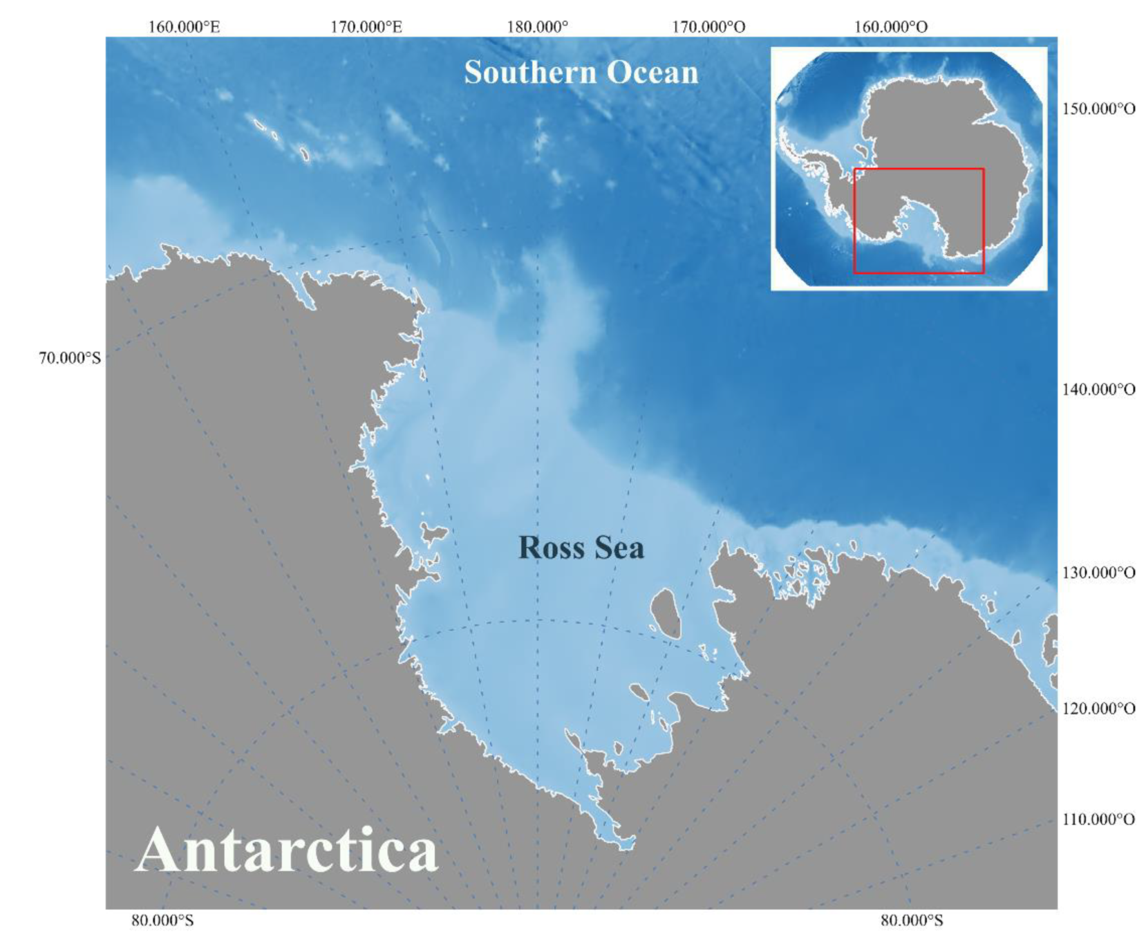
Following a pilot survey in 1989–1990, eight acoustic surveys targeting Antarctic krill (
Euphausia superba) and crystal krill (
Euphausia crystallorophias) in the western Ross Sea were conducted between 1994 and 2016, yielding some intriguing information on the krill populations of the Ross Sea [
7,
8,
9]. Taking into account ice coverage and krill spatial distribution, it was clearly evident that both
E. superba and
E. crystallorophias were concentrated around latitude 74° S in November, when ice coverage was quite dense and diffused. The situation differed in December-January when polynyas (ice-free areas) are typically much larger; both species traveled north, but to varying degrees, with
E. superba reaching farther north, close to the shelf break than
E. crystallorophias. These two species are probably in competition, having similar feeding appendages and a similar diet based primarily on phytoplankton [
10,
11], but with a non-negligible quota of zooplankton [
12,
13]. In the Ross Sea, however,
E. superba appears to prefer water mixing at the shelf break and continental slope, while
E. crystallorophias generally prefer shallow waters or areas close to ice [
8,
9], thus reducing overlap and competition for food.
There is evidence that environmental factors can influence krill populations around the Antarctic continent, resulting in changes in their abundance and spatial distribution [
4,
14]. For instance, phytoplankton blooms originating from ice melting through released algae appear to promote an increase in krill biomass [
15,
16]. Therefore, krill abundance may be locally favored by low salinity conditions and high chlorophyll
a concentration, which means ice melting and consequent phytoplankton bloom [
1]. Moreover, the ice edge may be a favorable environment for krill due to its high productivity conditions, also providing protection to early developmental stages from predators [
17,
18]. Other environmental factors, such as dissolved oxygen, especially if considered in conjunction with the general rise in temperature, which reduces the amount of oxygen in the water, with potential consequences for krill swarm formation and relative packing density, could also be important for krill dynamics [
19]. This factor may also represent a direct threat to the survival of these species [
20].
The Ross Sea has witnessed significant changes in recent years, including an increase in mean summer air temperature and a decrease in shelf water salinity from the 1950s to the present day [
21]. On a decadal time scale (1995–2006), these factors affected the formation of Antarctic Bottom Water (AABW) in the western and central Ross Sea [
22,
23], as well as Ice Shelf Water (ISW) and High Salinity Shelf Water (HSSW). All these changes, and eventually others, may have influenced the behavior of krill.
In this paper, we analyzed Antarctic krill and crystal krill biomass data and satellite environmental data to determine whether recent environmental changes have altered the abundance and distribution of E. superba and E. crystallorophias in the western Ross Sea. We also investigated the potential ramifications for other levels of the local pelagic food web.
3. Results
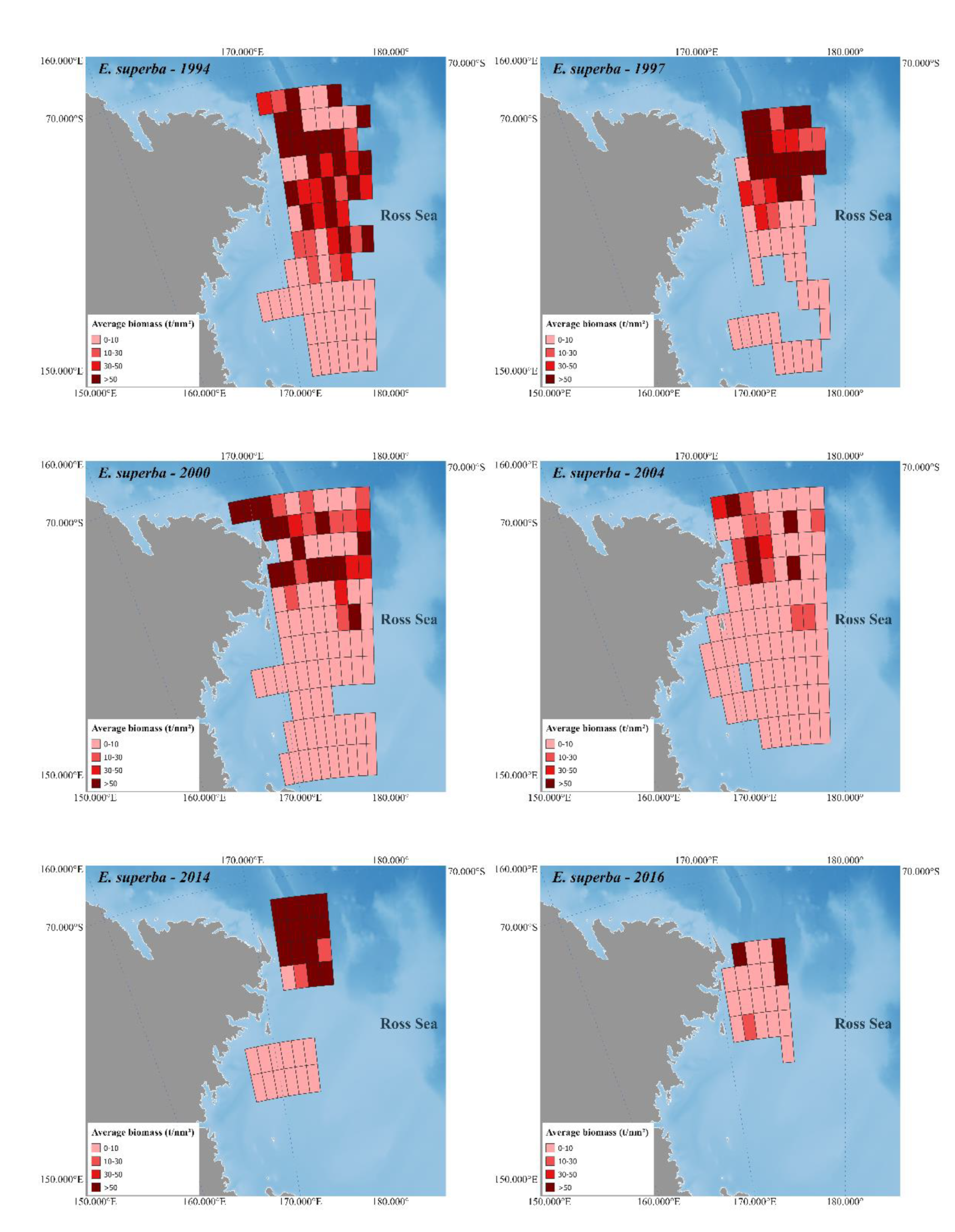
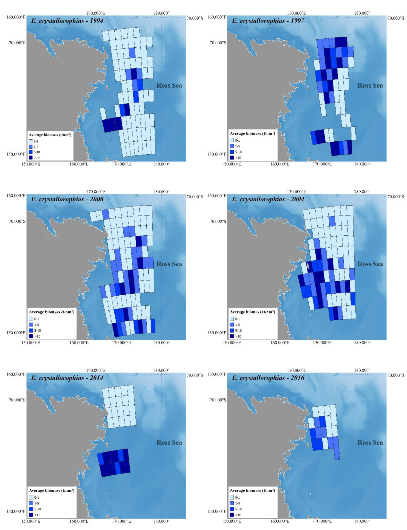
Figure 2 and
Figure 3 depict Antarctic krill and crystal krill biomass, respectively, estimated acoustically for the ESSR covered by the six surveys held in the western Ross Sea. The bathymetry reference for these figures is [
47], while the land is based on [
48].
3.1. Mean Environmental Data in the Water Column Relevant for Krill Biomass Estimation (0–200 m)
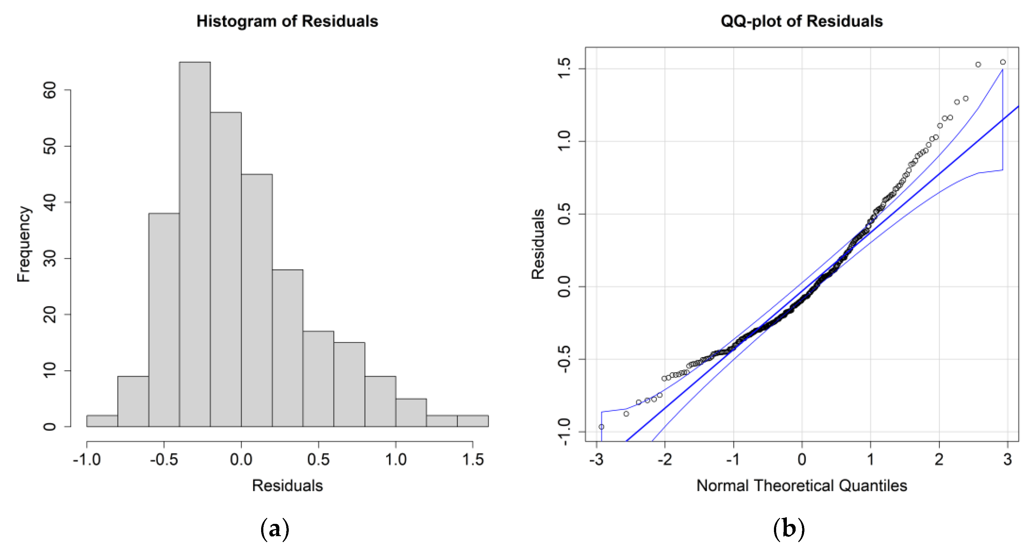
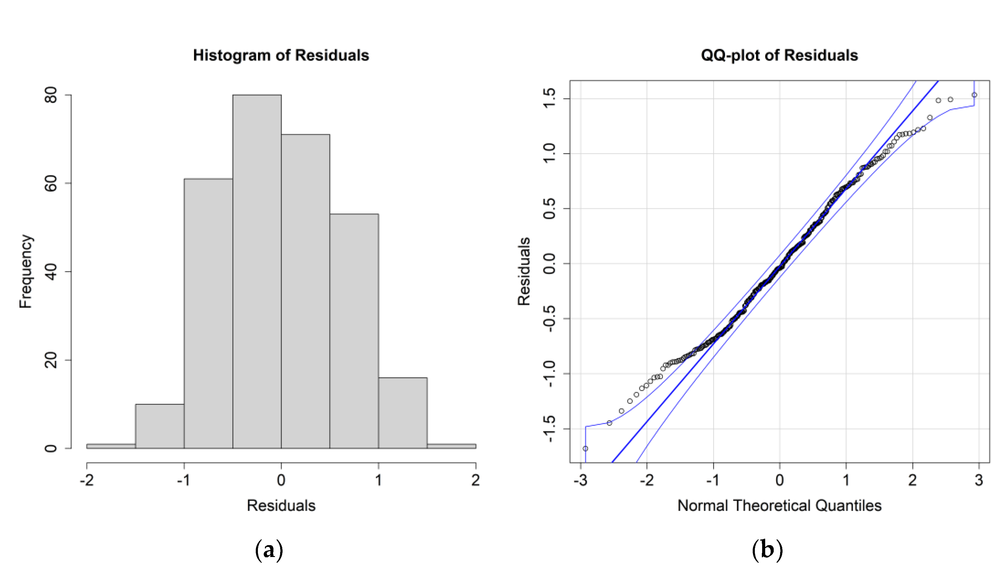
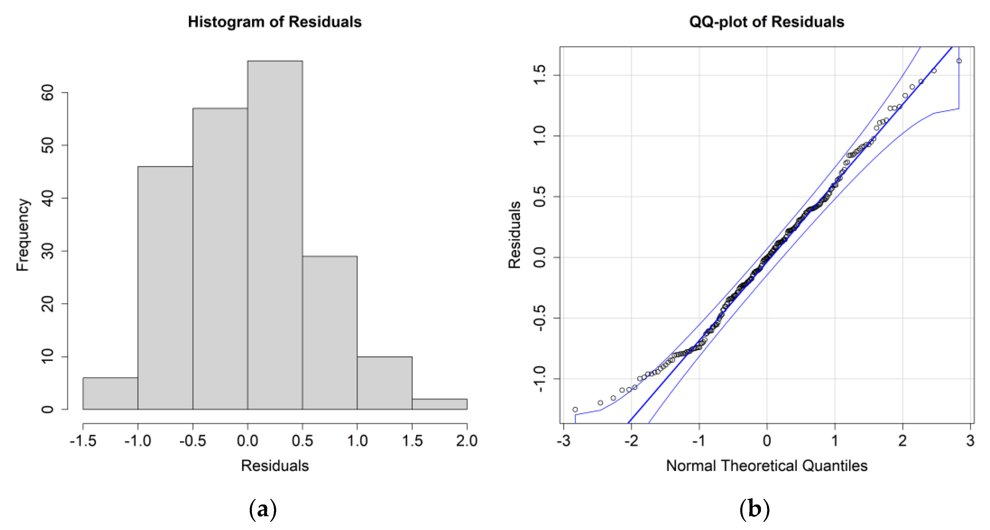
The ANOVA results for
E. crystallorophias, leaving the significant environmental parameters, are reported in
Table 2, while the residuals’ histograms and QQ plots are shown in
Figure 4.
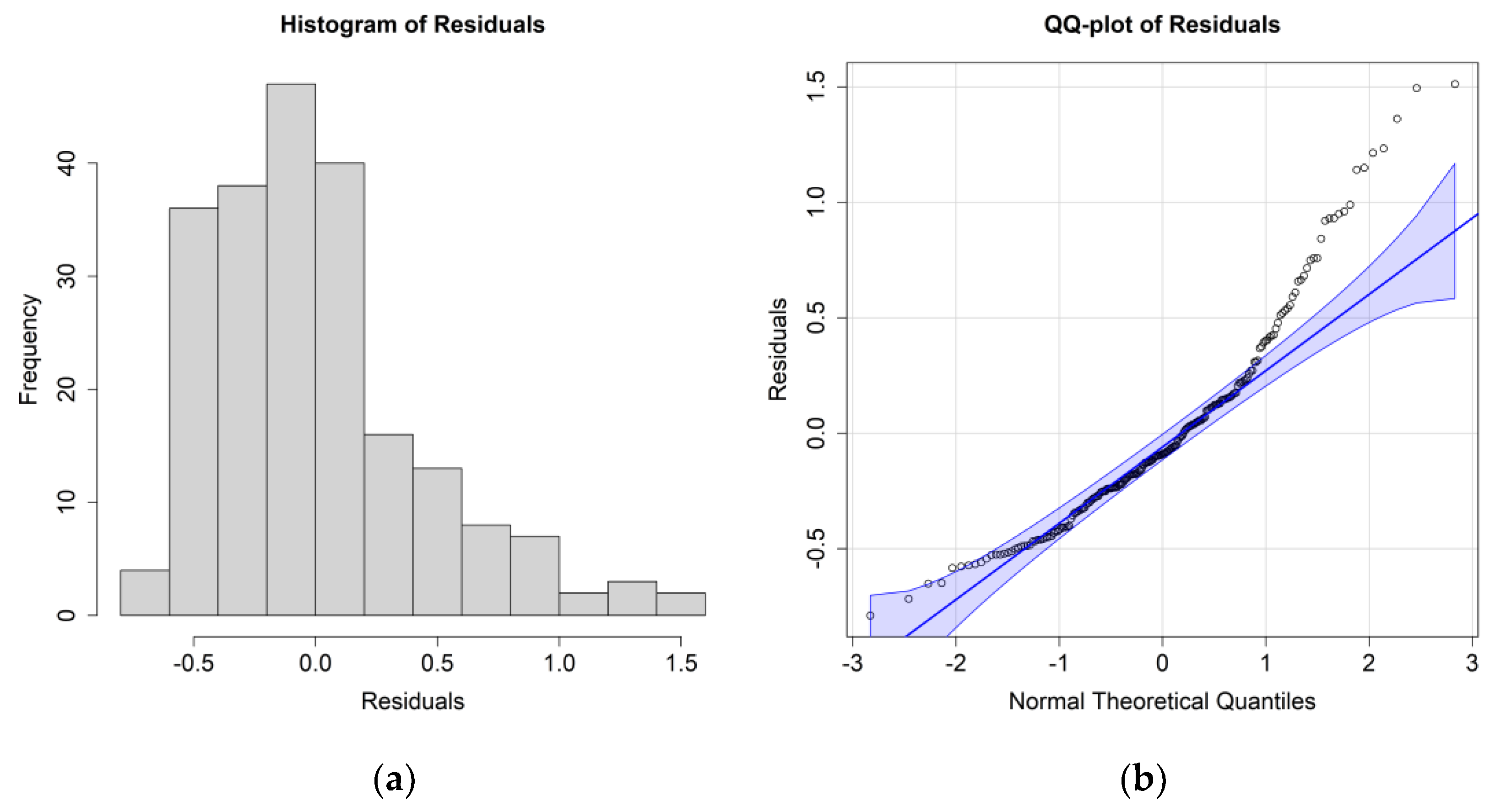
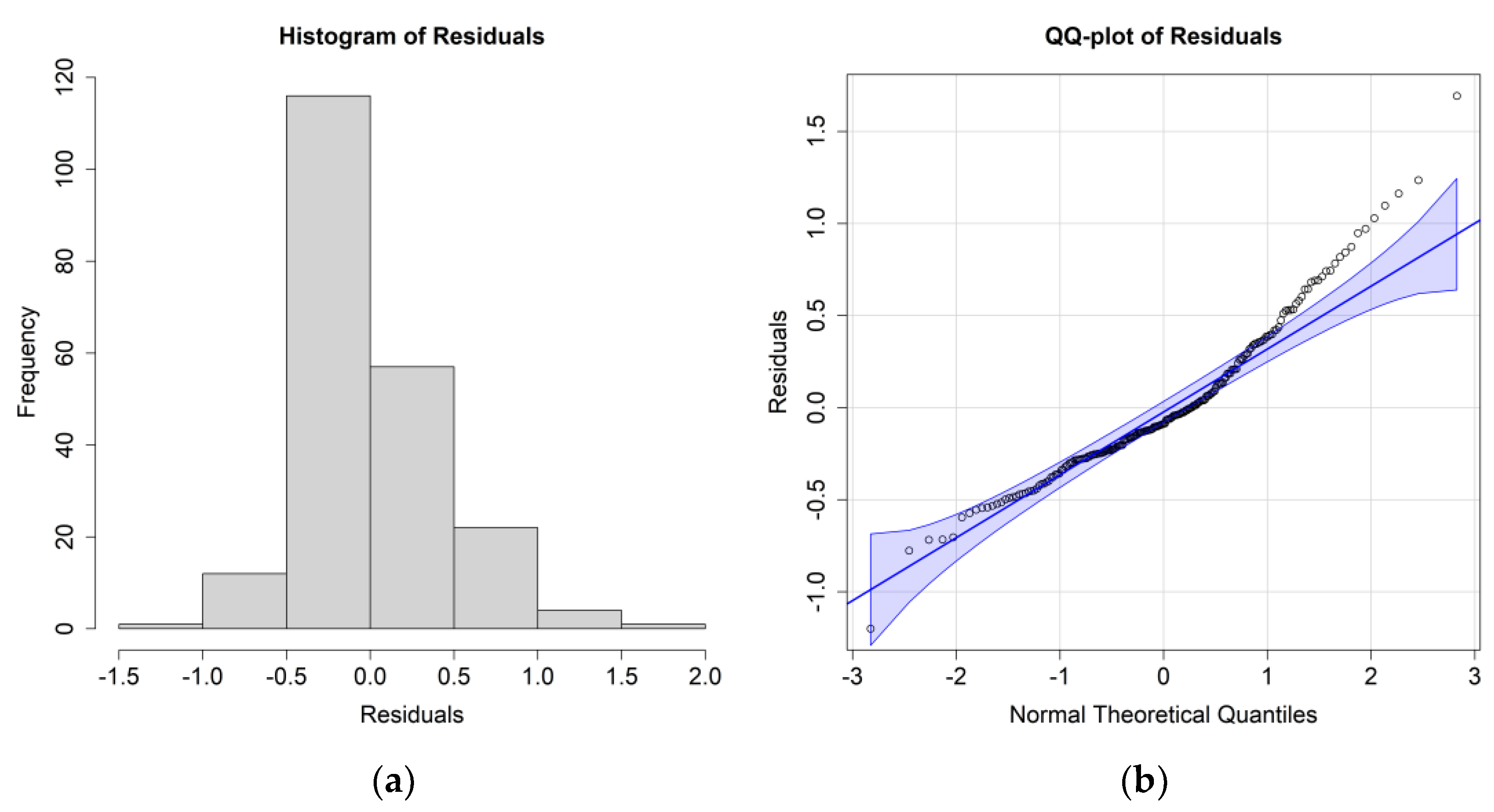
The ANOVA results for
E. superba, including only the significant environmental parameters, are reported in
Table 3; residuals’ histograms and QQ plots are shown in
Figure 5.
To summarize the most important results, crystal krill biomass presented highly statistically significant correlations with the survey year, ice coverage, and dissolved oxygen, whereas significant correlations were found with salinity. Antarctic krill showed highly significant correlations with the survey month, survey year, chlorophyll a concentration, and dissolved oxygen, whereas significant correlations were found with salinity and water velocity. This indicates that both species are sensitive to dissolved oxygen levels and that their biomass has altered over the years. As regards crystal krill, ice coverage also seems to be important, while the E. superba biomass has a significant association with chlorophyll a concentration and the survey month.
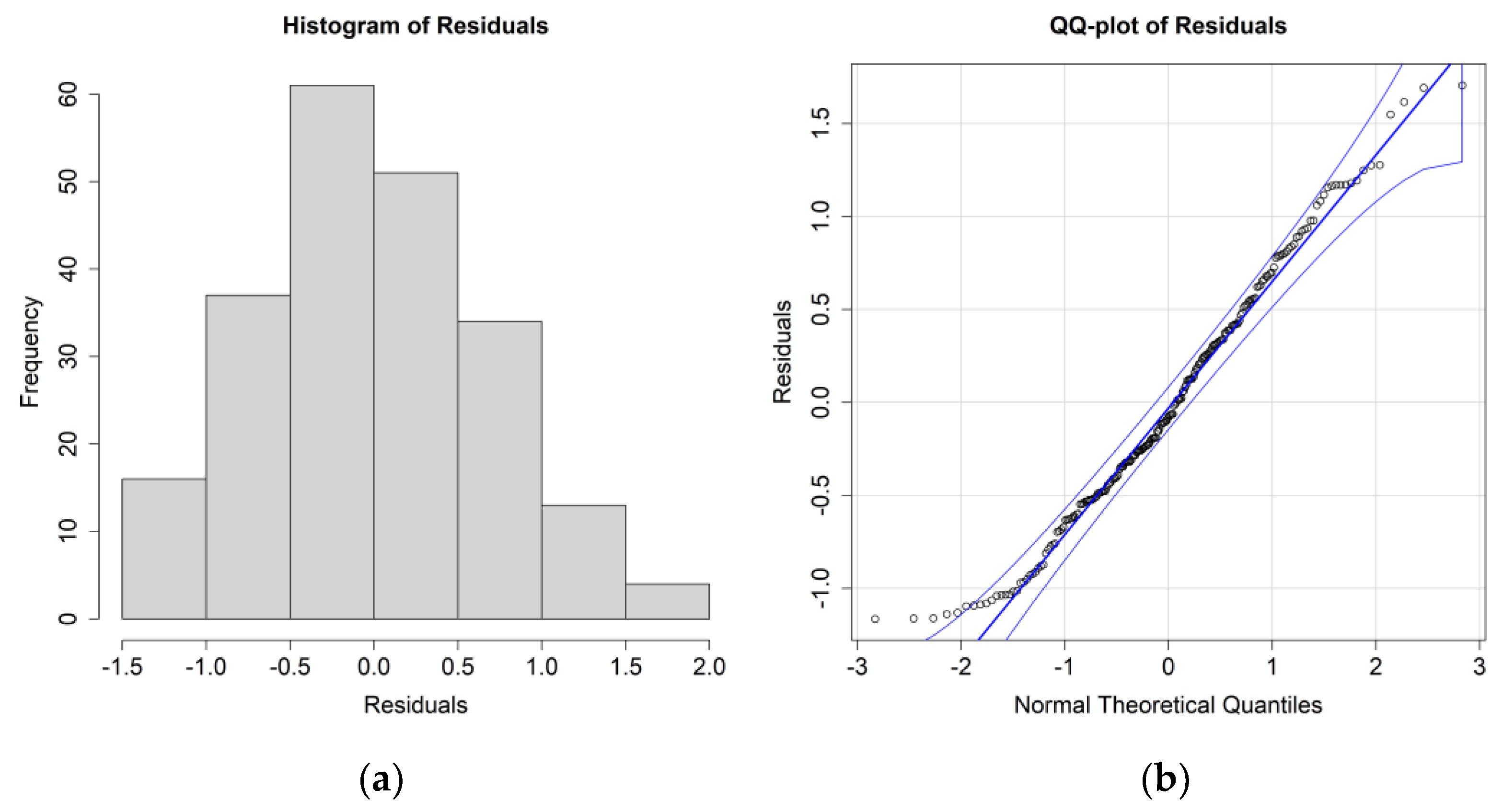
3.2. Environmental Data at the Surface Layer (0.5 m)
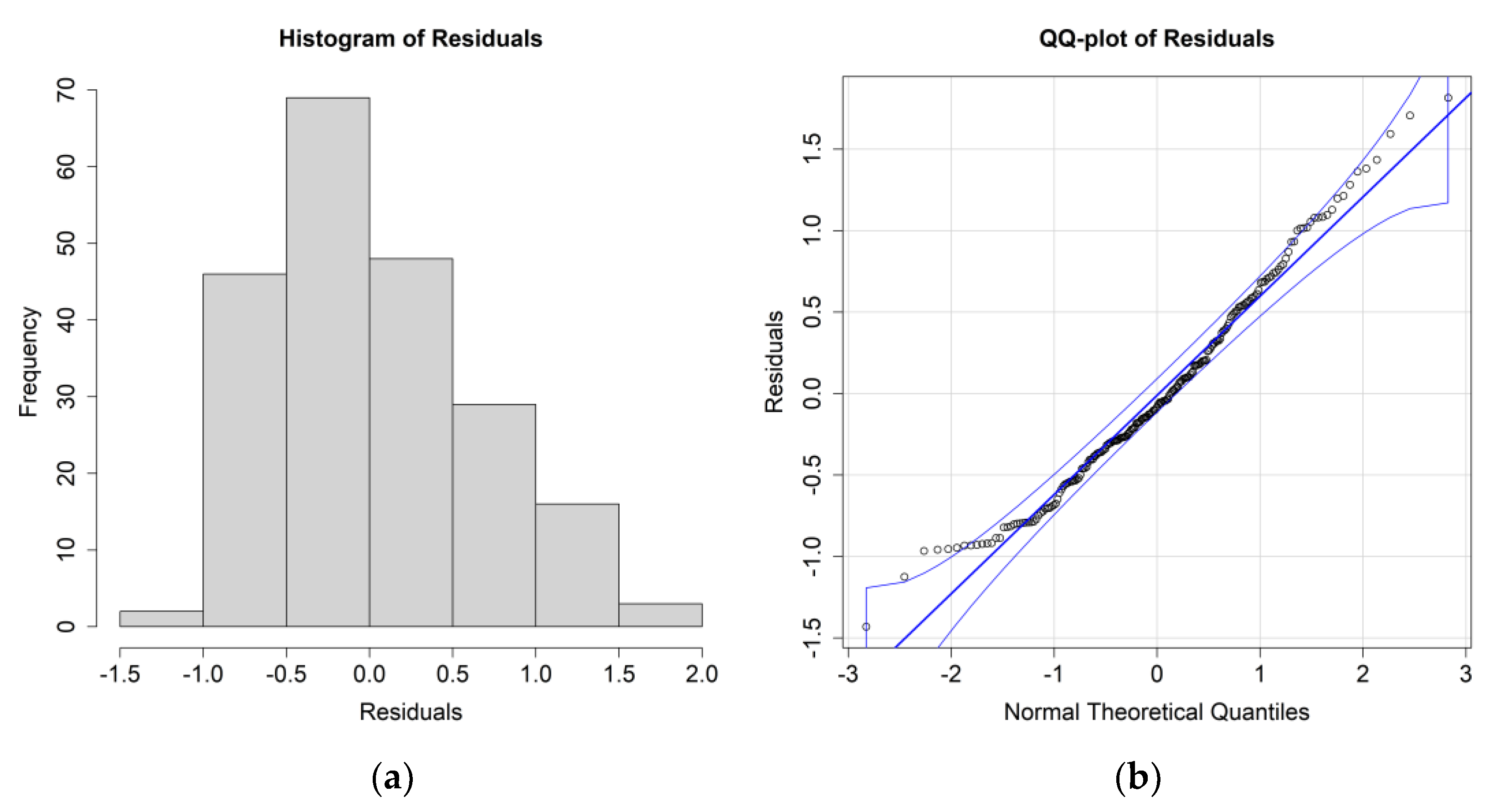
The
E. crystallorophias ANOVA results for this case study are reported in
Table 4, while the residuals’ histograms and QQ plot are reported in
Figure 6.
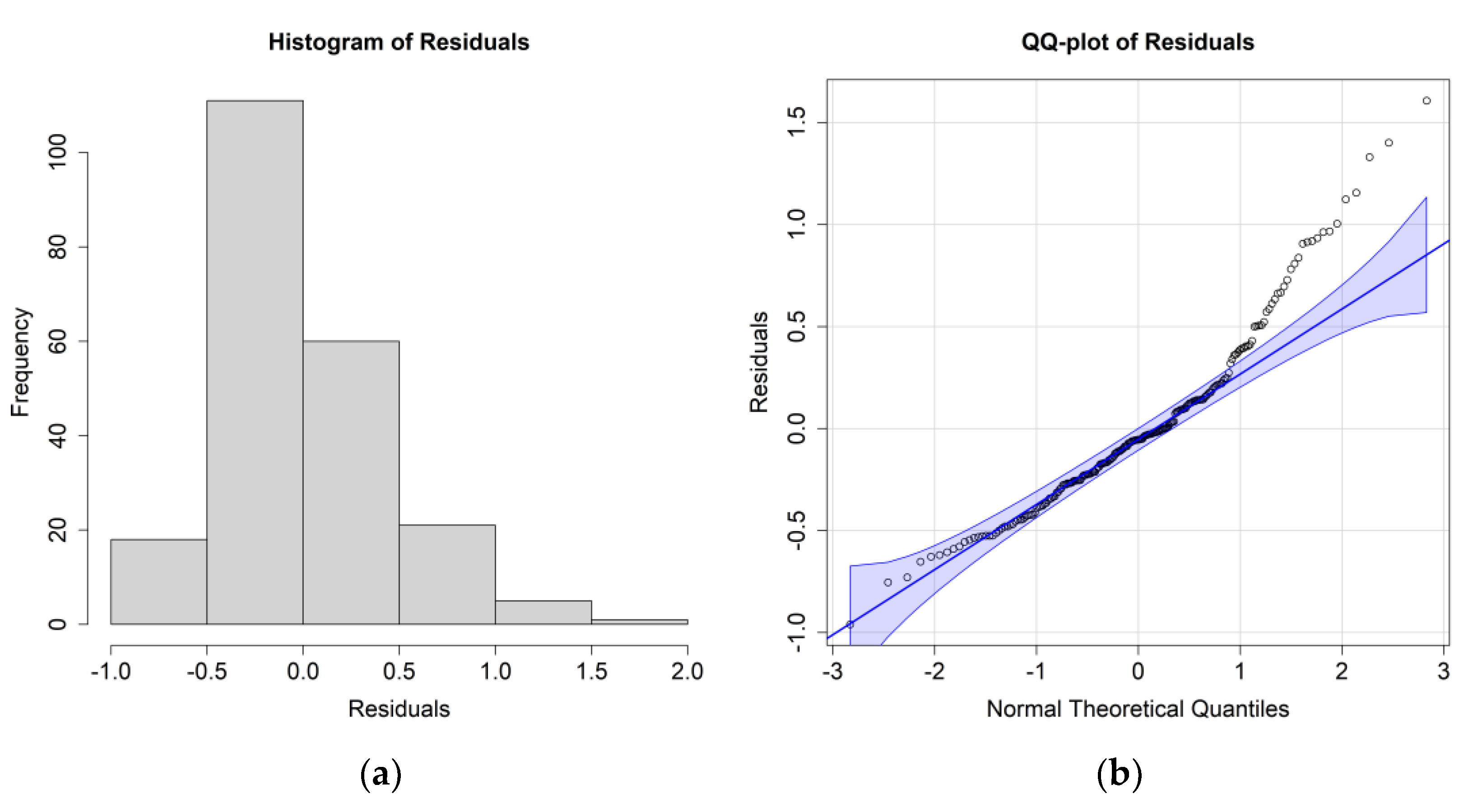
The
E. superba ANOVA results analyzed together with environmental parameters at the surface layer are reported in
Table 5; residuals’ histograms and QQ plots are shown in
Figure 7.
Crystal krill biomass presented highly significant connections with temperature and significant correlations with the survey year and chlorophyll a concentration. Antarctic krill exhibited highly significant connections with the survey month, survey year, and temperature, while a significant correlation was found with salinity. At the surface layer, both species were shown to be influenced by temperature, with Antarctic krill biomass being the only one to also vary in accordance with the survey year and month, as was the case for averaged environmental parameters throughout the water column.
3.3. Environmental Data at the 97 m Layer
The ANOVA results for the
E. crystallorophias case study are reported in
Table 6, while the histograms and QQ plots depicting residuals are reported in
Figure 8.
The
E. superba ANOVA results analyzed together with environmental parameters at the 97 m layer are reported in
Table 7; residuals’ histograms and QQ plots are shown in
Figure 9.
Temperature and dissolved oxygen were found to be highly significant for the E. crystallorophias biomass. E. superba exhibited highly significant correlations with the survey month and year, temperature, chlorophyll a concentration, and dissolved oxygen. At around 100 m depth, the factors that seem to exert the biggest influence are temperature and dissolved oxygen for both species. E. superba presented a highly significant connection with chlorophyll a concentration, survey month, and survey year. Other significant correlations for E. crystallorophias were found to be the survey year, water velocity, and chlorophyll concentration.
3.4. Environmental Data at the 199 m Layer
The ANOVA results for the
E. crystallorophias case study are reported in
Table 8, while the residuals’ histograms and QQ plot are depicted in
Figure 10.
The ANOVA results for
E. superba analyzed together with environmental parameters at the 199 m layer are reported in
Table 9; residuals’ histograms and QQ plots are shown in
Figure 11.
Temperature and phytoplankton correlations with the E. crystallorophias biomass were found to be highly significant. E. superba showed highly significant associations with the survey month, survey year, and temperature. At a depth of 200 m, temperature appears to influence both species. Phytoplankton concentration seems to be important for crystal krill, while the survey month and year influence Antarctic krill. Other significant connections were found with the survey year and chlorophyll a concentration for E. crystallorophias, as well as chlorophyll concentration in the case of E. superba.
All the above results, limited to highly significant correlations, are summarized in
Table 10.
The results of Levene’s test and the Tukey test for each of the above case studies can be found in the
Supplementary Materials.
4. Discussion
Crystal krill yielded very different results when environmental average values from 0 to 200 m were compared to values at fixed depth strata. In the former case, the most significant correlations involve the survey year, ice coverage, and dissolved oxygen. However, when fixed depth strata are considered, the variable most strongly correlated with krill biomass is temperature, followed by dissolved oxygen at a depth of 100 m and total phytoplankton concentration at a depth of 200 m. The correlation between the survey year and crystal krill biomass in the western Ross Sea suggests that the biomass has varied significantly across the years in which the surveys were conducted. Previous studies have revealed a correlation between
E. crystallorophias biomass and ice coverage [
9,
49], as this species prefers to inhabit coastal and ice-covered areas and should be sensitive to ice dynamics. The relationship between crystal krill and sea ice can be explained by the availability of food and the desire to protect eggs and early life stages [
50,
51,
52].
As regards the synergistic relationship between temperature and dissolved oxygen, we have already mentioned a general rise in water temperature in the Ross Sea, which would result in a decrease in the water’s oxygen concentration. This may have a deleterious impact on krill swarm formation and relative density [
19], posing a potential threat to these species’ survival rate [
20]. Based on our results, this synergistic effect on crystal krill should be stronger at a depth of around 100 m. In all fixed strata analyses, the temperature is by far the most prominent environmental parameter with significant connections in the case of crystal krill. This factor may be related to the importance of temperature in the regulation of krill metabolism [
53]. Some experiments [
54] demonstrated that food and oxygen demands tend to increase as temperatures rise, with a possible subtraction of energy from other activities, such as reproduction, in a global warming scenario such as the one we are helping to create. Temperature is also important for the stabilization of ice coverage, given that ice is important as a reserve of food and shelter for the protection of krill larvae [
55,
56,
57,
58]. Moreover, ice-free areas often demonstrate the predominance of krill rivals such as
Salpa thompsoni [
57]. Optimal summer temperatures seem to differ for these two krill species, with
E. superba preferring higher temperatures at the shelf break in the northern part of the Ross Sea and
E. crystallorophias preferring the shallower depths and colder temperatures of the south-western neritic part [
8,
9,
50]. At least during the austral summer, this factor contributes to the spatial separation of these species and significantly reduces competition for food. The link between crystal krill abundance and phytoplankton has already been the subject of prior research [
1,
9]; however, the significance of its availability at greater depths (200 m), as demonstrated in this study, may not be as well documented. As also reported in other Antarctic areas [
58], our data revealed that this species is quite abundant even at 100 m or more. For this reason, crystal krill at depths between 100–200 m could be quite influenced by the availability of phytoplankton in these or neighboring strata above.
In the ANOVA results, Antarctic krill presented a main difference with respect to crystal krill: the survey month and survey year had significant correlations with biomass in all case studies. This factor highlights the considerable variability of Antarctic krill biomass over the years, as well as a major difference between the situation in December, when ice is denser, and January, when most of the area is typically ice-free. The different levels of abundance and spatial distribution of Antarctic krill between December and January, as discussed in this paper, were also reported in previous studies [
8,
9]. In fact, a comparison of the beginning of austral summer with full summer reveals quite a diverse picture for these creatures, with the bulk of Antarctic krill distribution shifting northwards throughout the summer period. Even in the case of Antarctic krill, temperature appears to be a highly significant parameter for similar reasons as those reported for crystal krill; analogous considerations may also be made in this case, but taking into account these two species’ different preferences. Another, less-studied phenomenon connected to the rise in temperature and consequent increase in ice melting, is the stranded Antarctic krill individuals found in certain regions of Antarctica, such as Potter Cove [
59], where the creatures’ guts were found to be full of particles suspended in the floods originating from melted ice. The latter is another example of the importance of a balance between temperature, ice presence, and marine organisms in Antarctic ecosystems. A significant association between
E. superba biomass and dissolved oxygen was observed in the average values of the first 200 m and the 100 m depth strata. This factor reinforces the notion that both these krill species are sensitive to the same environmental parameters, despite their different preference ranges, as observed for temperature. Similarly, chlorophyll
a concentration had an impact on Antarctic krill biomass when environmental parameters were averaged from 0 to 200 m and 100 m depth strata. This element highlights the trophic factor’s importance for Antarctic krill, particularly the availability of phytoplankton [
60,
61], in addition to boosting krill recruitment [
62]. The ANOVA results suggest that the 100 m depth stratum has the highest phytoplankton concentration. Looking at the CTD profiles reported in [
63], which were performed at the positions of pelagic hauls during the 2004 acoustic survey in the western Ross Sea, a peak in fluorescence can be seen at a 40–50 m depth, and in one case, even deeper. This suggests that chlorophyll concentration in these depth strata could exert a relevant influence on Antarctic krill. In any case, the analyses of fluorescence data from CTD sampling should be improved in order to support this hypothesis. Some authors also discovered an increase in Antarctic krill lipid reserves in conjunction with increasing levels of chlorophyll
a concentration, estimated from remote sensing data collection and a decrease in sea surface temperature [
11]. The present results showed significant associations between Antarctic krill biomass, chlorophyll
a concentration, and temperature at a depth of 100 m, suggesting that something similar to the reported instance could also have happened in our study.
This paper demonstrates that acoustic estimations of krill biomass combined with satellite-derived environmental data can provide intriguing insights into the environmental variables that exert an influence on krill and, consequently, the Ross Sea’s local pelagic ecosystem. These preliminary results may provide an avenue for expanding our understanding of the spatial and temporal variations of krill biomass in the Ross Sea. The inclusion of krill spatial distribution and data on krill recruitment and krill predators should improve the precision of these conclusions.


 ,
, 


