
Network Analysis Using Markov Chain Applied to Wildlife Habitat Selection

 , ,
, ,
Abstract
:1. Introduction
2. Materials and Methods
2.1. Movement Data
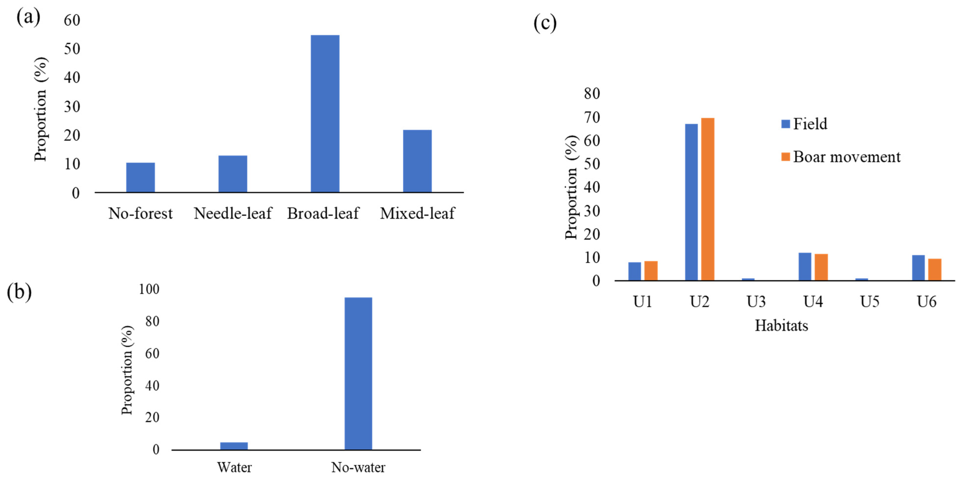
2.2. Habitat States
2.3. DTMC and Centrality
- -
- Degree centrality represents connectedness with other nodes and is calculated based on the number of connecting edges and weights for each node.
- -
- Betweenness centrality measures how many times each node appears on the shortest path between two nodes of the network.
- -
- Closeness centrality addresses the closeness of the target node to other nodes and is calculated as the sum of the lengths of the shortest paths between the nodes and all other nodes in the network.
3. Results
3.1. The Transition Probability Matrix (TPM)
3.2. Stationary State Transition Probabilities and Network Compositions
3.3. Hitting Time and Centrality
4. Discussion
5. Conclusions
Author Contributions
Funding
Institutional Review Board Statement
Informed Consent Statement
Data Availability Statement
Acknowledgments
Conflicts of Interest
Appendix A

| Id_Sex_Life Stage * | Observed Months | Recorded Points | Sources |
|---|---|---|---|
| #67M_Fer. | Feb, Mar | 407 | Collar |
| #67M_Peri. | May, Jun, Jul | 439 | Collar |
| #05M_Peri. | May, Jun | 378 | Web |
| #67M_Brood. | Aug, Sep, Oct | 529 | Collar |
| #06M_Brood. | Sep, Oct | 135 | Web |
| #68M_Brood. | Oct | 171 | Collar |
| #67M_Mati. | Nov, Dec, Jan | 675 | Collar |
| #68M_Mati. | Nov | 236 | Collar |
Appendix B

Appendix C
References
- Muheim, R.; Boström, J.; Åkesson, S.; Liedvogel, M. Sensory Mechanisms of Animal Orientation and Navigation. In Animal Movement Across Scales; Oxford University Press: Great Clarendon, UK, 2014; pp. 179–194. [Google Scholar]
- Fagan, W.F.; Lewis, M.A.; Auger-Méthé, M.; Avgar, T.; Benhamou, S.; Breed, G.; Ladage, L.; Schlägel, U.E.; Tang, W.W.; Papastamatiou, Y.P.; et al. Spatial Memory and Animal Movement. Ecol. Lett. 2013, 16, 1316–1329. [Google Scholar] [CrossRef] [PubMed]
- Morelle, K. Wild Boar Movement Ecology across Scales: Insights from a Population Expanding into Agroecosystems of Southern Belgium. Ph.D. Thesis, Université de Liège, Liège, Belgique, 2015. [Google Scholar]
- Turchin, P. Translating Foraging Movements in Heterogeneous Environments into the Spatial Distribution of Foragers. Ecology 1991, 72, 1253–1266. [Google Scholar] [CrossRef]
- Lange, M.; Guberti, V.; Thulke, H. Understanding ASF Spread and Emergency Control Concepts in Wild Boar Populations Using Individual-based Modelling and Spatio-temporal Surveillance Data. EFSA Support. Publ. 2018, 15. [Google Scholar] [CrossRef]
- Worton, B.J. A Review of Models of Home Range for Animal Movement. Ecol. Model. 1987, 38, 277–298. [Google Scholar] [CrossRef]
- Tang, W.; Bennett, D.A. Agent-Based Modeling of Animal Movement: A Review. Geogr. Compass 2010, 4, 682–700. [Google Scholar] [CrossRef]
- Smouse, P.E.; Focardi, S.; Moorcroft, P.R.; Kie, J.G.; Forester, J.D.; Morales, J.M. Stochastic Modelling of Animal Movement. Philos. Trans. R. Soc. B Biol. Sci. 2010, 365, 2201–2211. [Google Scholar] [CrossRef] [Green Version]
- Beck, J.L.; Suring, L.H. Wildlife Habitat-Relationships Models. In Models for Planning Wildlife Conservation in Large Landscapes; Elsevier: Amsterdam, The Netherlands, 2009; pp. 251–285. ISBN 9780123736314. [Google Scholar]
- Rho, P. Using Habitat Suitability Model for the Wild Boar (Sus Scrofa Linnaeus) to Select Wildlife Passage Sites in Extensively Disturbed Temperate Forests. J. Ecol. Environ. 2015, 38, 163–173. [Google Scholar] [CrossRef] [Green Version]
- Dettki, H.; Löfstrand, R.; Edenius, L. Modeling Habitat Suitability for Moose in Coastal Northern Sweden: Empirical vs Process-Oriented Approaches. AMBIO J. Hum. Environ. 2003, 32, 549–556. [Google Scholar] [CrossRef]
- Janeau, G.; Cargnelutti, B.; Cousse, S.; Hewison, M.; Spitz, F. Daily Movement Pattern Variations in Wild Boar (Sus scrofa L.). Ibex J. Mt. Ecol. 1995, 3, 98–101. [Google Scholar]
- Cherry, S. A Comparison of Confidence Interval Methods for Habitat Use-Availability Studies. J. Wildl. Manag. 1996, 60, 653. [Google Scholar] [CrossRef]
- Erdtmann, D.; Keuling, O. Behavioural Patterns of Free Roaming Wild Boar in a Spatiotemporal Context. PeerJ 2020, 8, e10409. [Google Scholar] [CrossRef] [PubMed]
- Rew, J.; Cho, Y.; Moon, J.; Hwang, E. Habitat Suitability Estimation Using a Two-Stage Ensemble Approach. Remote Sens. 2020, 12, 1475. [Google Scholar] [CrossRef]
- Kay, S.L.; Fischer, J.W.; Monaghan, A.J.; Beasley, J.C.; Boughton, R.; Campbell, T.A.; Cooper, S.M.; Ditchkoff, S.S.; Hartley, S.B.; Kilgo, J.C.; et al. Quantifying Drivers of Wild Pig Movement across Multiple Spatial and Temporal Scales. Mov. Ecol. 2017, 5, 14. [Google Scholar] [CrossRef] [PubMed] [Green Version]
- Blackwell, P.G.; Niu, M.; Lambert, M.S.; Lapoint, S.D. Exact Bayesian Inference for Animal Movement in Continuous Time. Methods Ecol. Evol. 2016, 7, 184–195. [Google Scholar] [CrossRef]
- Booth, T.H.; Nix, H.A.; Busby, J.R.; Hutchinson, M.F. Bioclim: The First Species Distribution Modelling Package, Its Early Applications and Relevance to Most Current MaxEnt Studies. Divers. Distrib. 2014, 20, 1–9. [Google Scholar] [CrossRef]
- Torney, C.J.; Morales, J.M.; Husmeier, D. A Hierarchical Machine Learning Framework for the Analysis of Large Scale Animal Movement Data. Mov. Ecol. 2021, 9, 6. [Google Scholar] [CrossRef]
- Carroll, K.A.; Hansen, A.J.; Inman, R.M.; Lawrence, R.L. Evaluating the Importance of Wolverine Habitat Predictors Using a Machine Learning Method. J. Mammal. 2021, 106, 1466–1472. [Google Scholar] [CrossRef]
- Bosch, J.; Mardones, F.; Pérez, A.; de la Torre, A.; Muñoz, M.J. A Maximum Entropy Model for Predicting Wild Boar Distribution in Spain. Span. J. Agric. Res. 2014, 12, 984–999. [Google Scholar] [CrossRef] [Green Version]
- Patterson, T.A.; Thomas, L.; Wilcox, C.; Ovaskainen, O.; Matthiopoulos, J. State–Space Models of Individual Animal Movement. Trends Ecol. Evol. 2008, 23, 87–94. [Google Scholar] [CrossRef]
- Patterson, T.A.; Basson, M.; Bravington, M.v.; Gunn, J.S. Classifying Movement Behaviour in Relation to Environmental Conditions Using Hidden Markov Models. Journal of Animal Ecology 2009, 78, 1113–1123. [Google Scholar] [CrossRef]
- McClintock, B.T.; Langrock, R.; Gimenez, O.; Cam, E.; Borchers, D.L.; Glennie, R.; Patterson, T.A. Uncovering Ecological State Dynamics with Hidden Markov Models. Ecol. Lett. 2020, 23, 1878–1903. [Google Scholar] [CrossRef] [PubMed]
- Blackwell, P.G. Random Diffusion Models for Animal Movement. Ecol. Model. 1997, 100, 87–102. [Google Scholar] [CrossRef]
- Lange, M.; Thulke, H.H. Elucidating Transmission Parameters of African Swine Fever through Wild Boar Carcasses by Combining Spatio-Temporal Notification Data and Agent-Based Modelling. Stoch. Environ. Res. Risk Assess. 2017, 31, 379–391. [Google Scholar] [CrossRef]
- Railsback, S.F.; Harvey, B.C. Analysis of Habitat-Selection Rules Using an Individual-Based Model. Ecology 2002, 83, 1817. [Google Scholar] [CrossRef]
- DeAngelis, D.L.; Grimm, V. Individual-Based Models in Ecology after Four Decades. F1000Prime Rep. 2014, 6, 39. [Google Scholar] [CrossRef] [Green Version]
- Newman, M. Networks: An Introduction. In Netw: An Introduction; Oxford Scholarship: Oxford, UK, 2010; pp. 1–784. [Google Scholar] [CrossRef] [Green Version]
- Da Mata, A.S. Complex Networks: A Mini-Review. Braz. J. Phys. 2020, 50, 658–672. [Google Scholar] [CrossRef]
- Dale, M.R.T.; Fortin, M.J. From Graphs to Spatial Graphs. Annu. Rev. Ecol. Evol. Syst. 2010, 41, 21–38. [Google Scholar] [CrossRef]
- Saxena, A.; Iyengar, S. Centrality Measures in Complex Networks: A Survey. arXiv 2020, arXiv:2011.07190. [Google Scholar]
- Balcan, D.; Colizza, V.; Gonçalves, B.; Hu, H.; Ramasco, J.J.; Vespignani, A. Multiscale Mobility Networks and the Spatial Spreading of Infectious Diseases. PNAS Dec. 2009, 22, 21484–21489. [Google Scholar] [CrossRef] [Green Version]
- Wey, T.; Blumstein, D.T.; Shen, W.; Jordán, F.; Jordán, J. Social Network Analysis of Animal Behaviour: A Promising Tool for the Study of Sociality. Anim. Behav. 2008, 75, 333–344. [Google Scholar] [CrossRef]
- Silk, M.J.; Fisher, D.N. Understanding Animal Social Structure: Exponential Random Graph Models in Animal Behaviour Research. Anim. Behav. 2017, 132, 137–146. [Google Scholar] [CrossRef] [Green Version]
- Podgórski, T. Effect of Relatedness on Spatial and Social Structure of the Wild Boar Sus Scrofa Population in Białowieża Primeval Forest. Ph.D. Thesis, University of Warsaw, Faculty of Biology, Białowieża, Poland, 2013. [Google Scholar]
- Pătru-Stupariu, I.; Nita, A.; Mustăţea, M.; Huzui-Stoiculescu, A.; Fürst, C. Using Social Network Methodological Approach to Better Understand Human–Wildlife Interactions. Land Use Policy 2020, 99, 105009. [Google Scholar] [CrossRef]
- Pereira, J. Multi-Node Protection of Landscape Connectivity: Habitat Availability and Topological Reachability. Community Ecol. 2018, 19, 176–185. [Google Scholar] [CrossRef]
- Hilty, J.; Worboys, G.L.; Keeley, A.; Woodley, S.; Lausche, B.; Locke, H.; Carr, M.; Pulsford, I.; Pittock, J.; White, J.W.; et al. Guidelines for Conserving Connectivity through Ecological Networks and Corridors; Best Practice Protected Area Guidelines Series No. 30; IUCN: Gland, Switzerland, 2020. [Google Scholar]
- Walsh, M.G.; Mor, S.M. Interspecific Network Centrality, Host Range and Early-Life Development Are Associated with Wildlife Hosts of Rift Valley Fever Virus. Transbound. Emerg. Dis. 2018, 65, 1568–1575. [Google Scholar] [CrossRef] [PubMed]
- Bellini, S.; Scaburri, A.; Tironi, M.; Calò, S. Analysis of Risk Factors for African Swine Fever in Lombardy to Identify Pig Holdings and Areas Most at Risk of Introduction in Order to Plan Preventive Measures. Pathogens 2020, 9, 1077. [Google Scholar] [CrossRef] [PubMed]
- Murray, J.D. Mathematical Biology: I. An Introduction, 3rd ed.; Springer: Berlin/Heidelberg, Germany, 2002; pp. 1–576. [Google Scholar]
- Jacoby, D. A Network Analysis Approach to Understanding Shark Behaviour. Ph.D. Thesis, University of Exeter, Exeter, UK, 2012. [Google Scholar]
- Seo, E.; Hutchinson, R.A.; Fu, X.; Li, C.; Hallman, T.A.; Kilbride, J.; Robinson, W.D. StatEcoNet: Statistical Ecology Neural Networks for Species Distribution Modeling. arXiv 2021, arXiv:2102.08534. [Google Scholar]
- Kabak, I.W. Wildlife Management: An Application of a Finite Markov Chain. Am. Stat. 1970, 24, 27–29. [Google Scholar] [CrossRef]
- Metz, H.A.J.; Dienske, H.; de Jonge, G.; Putters, F.A. Continuous-Time Markov Chains as Models for Animal Behaviour. Bull. Math. Biol. 1983, 45, 643–658. [Google Scholar] [CrossRef]
- Wilson, K.; Hanks, E.; Johnson, D. Estimating Animal Utilization Densities Using Continuous-Time Markov Chain Models. Methods Ecol. Evol. 2018, 9, 1232–1240. [Google Scholar] [CrossRef] [Green Version]
- Whitehead, H.; Jonsen, I.D. Inferring Animal Densities from Tracking Data Using Markov Chains. PLoS ONE 2013, 8, e60901. [Google Scholar] [CrossRef] [Green Version]
- Spence, M.A.; Muiruri, E.W.; Maxwell, D.L.; Davis, S.; Sheahan, D. The Application of Continuous-Time Markov Chain Models in the Analysis of Choice Flume Experiments. J. R. Stat. Soc. Ser. C 2021, 70, 1103–1123. [Google Scholar] [CrossRef]
- De Arruda, G.F.; Rodrigues, F.A.; Rodríguez, P.M.; Cozzo, E.; Moreno, Y. A General Markov Chain Approach for Disease and Rumour Spreading in Complex Networks. J. Complex Netw. 2018, 6, 215–242. [Google Scholar] [CrossRef] [Green Version]
- Villarreal-Calva, R.C.; Escamilla-Ambrosio, P.J.; Rodríguez-Mota, A.; Ramírez-Cortés, J.M. Evolution of COVID-19 Patients in Mexico City Using Markov Chains. Commun. Comput. Inf. Sci. 2020, 1280, 309–318. [Google Scholar] [CrossRef]
- McClintock, B.T.; King, R.; Thomas, L.; Matthiopoulos, J.; McConnell, B.J.; Morales, J.M. A General Discrete-Time Modeling Framework for Animal Movement Using Multistate Random Walks. Ecol. Monogr. 2012, 82, 335–349. [Google Scholar] [CrossRef] [Green Version]
- Martin, M.; Béjar, J.; Esposito, G.; Chávez, D.; Contreras-Hernández, E.; Glusman, S.; Cortés, U.; Rudomín, P. Markovian Analysis of the Sequential Behavior of the Spontaneous Spinal Cord Dorsum Potentials Induced by Acute Nociceptive Stimulation in the Anesthetized Cat. Front. Comput. Neurosci. 2017, 11, 32. [Google Scholar] [CrossRef] [Green Version]
- Maw, S.Z.; Zin, T.T.; Tin, P.; Kobayashi, I.; Horii, Y. An Absorbing Markov Chain Model to Predict Dairy Cow Calving Time. Sensors 2021, 21, 6490. [Google Scholar] [CrossRef]
- Yang, H.C.; Chao, A. Modeling Animals’ Behavioral Response by Markov Chain Models for Capture-Recapture Experiments. Biometrics 2005, 61, 1010–1017. [Google Scholar] [CrossRef]
- Prasad, B.R.G.; Borges, R.M. Searching on Patch Networks Using Correlated Random Walks: Space Usage and Optimal Foraging Predictions Using Markov Chain Models. J. Theor. Biol. 2006, 240, 241–249. [Google Scholar] [CrossRef] [PubMed]
- Tejada, J.; Bosco, G.G.; Morato, S.; Roque, A.C. Characterization of the Rat Exploratory Behavior in the Elevated Plus-Maze with Markov Chains. J. Neurosci. Methods 2010, 193, 288–295. [Google Scholar] [CrossRef]
- Du Preez, B.; Hart, T.; Loveridge, A.J.; Macdonald, D.W. Impact of Risk on Animal Behaviour and Habitat Transition Probabilities. Anim. Behav. 2015, 100, 22–37. [Google Scholar] [CrossRef]
- Cruz-Angón, A.; Angón, A.; Sillett, T.S.; Greenberg, R. An experimental study of habitat selection by birds in a coffee plantation. Ecology 2008, 89, 921–927. [Google Scholar] [CrossRef] [PubMed]
- Tischendorf, L.; Wissel, C. Corridors as Conduits for Small Animals: Attainable Distances Depending on Movement Pattern, Boundary Reaction and Corridor Width. Oikos 1997, 79, 603. [Google Scholar] [CrossRef] [Green Version]
- IUCN. Natural Protected Areas of Republic of Korea; IUCN: Seoul, Korea, 2008. [Google Scholar]
- Aldridge, H.D.J.N.; Brigham, R.M. Load Carrying and Maneuverability in an Insectivorous Bat: A Test of the 5% “Rule” of Radio-Telemetry. J. Mammal. 1988, 69, 379–382. [Google Scholar] [CrossRef]
- Sikes, R.S.; The Animal Care and Use Committee of the American Society of Mammalogists. 2016 Guidelines of the American Society of Mammalogists for the Use of Wild Mammals in Research and Education. J. Mammal. 2016, 97, 663–688. [Google Scholar] [CrossRef] [PubMed]
- Boitani, L.; Mattei, L.; Nonis, D.; Corsi, F. Spatial and Activity Patterns of Wild Boars in Tuscany, Italy. J. Mammal. 1994, 75, 600–612. [Google Scholar] [CrossRef]
- Rosell, C.; Navàs, F.; Romero, S. Reproduction of Wild Boar in a Cropland and Coastal Wetland Area: Implications for Management. Anim. Biodivers. Conserv. 2012, 35, 209–217. [Google Scholar] [CrossRef]
- QGIS Development Team Welcome to the QGIS Project! Available online: https://www.qgis.org/en/site/ (accessed on 6 April 2021).
- Ministry of Environment. Environmental Geospatial Information Service; Government of the Republic of Korea: Seoul, Korea, 2021.
- Jurgiel, B. Point Sampling Tool-QGIS Python Plugins Repository. Version 0.5.3. 2020. Available online: https://plugins.qgis.org/plugins/pointsamplingtool/ (accessed on 31 March 2021).
- Grebner, D.L.; Bettinger, P.; Siry, J.P. Forest Products. In Introduction to Forestry and Natural Resources; Elsevier: Amsterdam, The Netherlands, 2013; Volume 30, pp. 97–124. [Google Scholar]
- Lee, S.M.; Lee, E.J. Diet of the Wild Boar (Sus Scrofa): Implications for Management in Forest-Agricultural and Urban Environments in South Korea. PeerJ 2019, 2019. [Google Scholar] [CrossRef] [Green Version]
- Abaigar, T.; del Barrio, G.; Vericad, J.R. Habitat Preference of Wild Boar (Sus Scrofa l., 1758) in a Mediterranean Environment. Indirect Evaluation by Signs. Mammalia 1994, 58, 201–210. [Google Scholar] [CrossRef]
- Erickson, R.V. Functions of Markov Chains. Ann. Math. Statist. 1970, 41, 843–850. [Google Scholar] [CrossRef]
- Gagniuc, P.A. Markov Chains: From Theory to Implementation and Experimentation; John Wiley & Sons: Hoboken, NJ, USA, 2017; ISBN 978-1-119-38759-6. [Google Scholar]
- Brémaud, P. Markov Chains Gibbs Fields, Monte Carlo Simulation and Queues; Texts in Applied Mathematics; Springer International Publishing: Cham, Germany, 2020; Volume 31, ISBN 978-3-030-45981-9. [Google Scholar]
- Matlab, Discrete-Time Markov Chains-MATLAB & Simulink. Available online: https://www.mathworks.com/help/econ/discrete-time-markov-chains.html (accessed on 31 March 2021).
- Matlab, Two-Sample Kolmogorov-Smirnov Test. The MathWorks, Inc.. 2021. Available online: https://www.mathworks.com/company/newsroom/mathworks-introduces-release-2021b-of-matlab-and-simulink.html (accessed on 31 March 2021).
- CentiServer Centralities List. Available online: https://www.centiserver.org (accessed on 1 April 2021).
- Matlab, Measure Node Importance-MATLAB Centrality. Available online: https://www.mathworks.com/help/matlab/ref/graph.centrality.html (accessed on 9 April 2021).
- Jacobs, J. Quantitative Measurement of Food Selection. Oecologia 1974, 14, 413–417. [Google Scholar] [CrossRef]
- Lewis, J.S.; Farnsworth, M.L.; Burdett, C.L.; Theobald, D.M.; Gray, M.; Miller, R.S. Biotic and Abiotic Factors Predicting the Global Distribution and Population Density of an Invasive Large Mammal. Sci. Rep. 2017, 7, 44152. [Google Scholar] [CrossRef] [PubMed]
- Hansen, B.; Reich, P.; Lake, P.S.; Cavagnaro, T. Minimum Width Requirements for Riparian Zones to Protect Flowing Waters and to Conserve Biodiversity: A Review and Recommendations; Report to the Office of Water; Victorian Department of Sustainability and Environment, Monash University: Melbourne, Australia, 2010; p. 150. [Google Scholar]


| Forest | No Forest | ||
|---|---|---|---|
| Broadleaf | Needleleaf | ||
| Water | U1 | U3 | U5 |
| No water | U2 | U4 | U6 |
| t * + 1 | U1 | U2 | U3 | U4 | U5 | U6 | n | U1 | U2 | U3 | U4 | U5 | U6 | n | ||||
|---|---|---|---|---|---|---|---|---|---|---|---|---|---|---|---|---|---|---|
| t | ||||||||||||||||||
| (a) | U1 | 46 | 43 | - | 7 | - | 4 | 29 | (e) | 26 | 51 | 0 | 12 | 0 | 11 | 57 |  | |
| U2 | 4 | 84 | - | 8 | - | 4 | 291 | 17 | 71 | 0 | 7 | 0 | 5 | 188 | ||||
| U3 | - | - | - | - | - | - | - | 0 | 0 | 0 | 100 | 0 | 0 | 1 | ||||
| U4 | 4 | 46 | - | 50 | - | 0 | 48 | 7 | 13 | 1 | 78 | 0 | 1 | 107 | ||||
| U5 | - | - | - | - | - | - | - | 50 | 0 | 0 | 50 | 0 | 0 | 2 | ||||
| U6 | 3 | 31 | - | 0 | - | 66 | 39 | 13 | 48 | 0 | 4 | 9 | 26 | 23 | ||||
| Average | 14 | 51 | - | 16 | - | 19 | Σ 407 | 19 | 31 | 0 | 42 | 2 | 7 | Σ 378 | ||||
| (b) | U1 | 24 | 55 | 0 | 8 | 0 | 13 | 38 | (f) | 8 | 77 | - | - | 8 | 7 | 13 | ||
| U2 | 7 | 76 | 0 | 11 | 0 | 6 | 296 | 7 | 85 | - | - | 0 | 8 | 110 | ||||
| U3 | 0 | 0 | 0 | 100 | 0 | 0 | 1 | - | - | - | - | - | - | - | ||||
| U4 | 6 | 47 | 0 | 42 | 0 | 5 | 66 | - | - | - | - | - | - | - | ||||
| U5 | 0 | 0 | 50 | 0 | 50 | 0 | 3 | 100 | 0 | - | - | 0 | 0 | 1 | ||||
| U6 | 9 | 51 | 0 | 6 | 5 | 29 | 35 | 27 | 55 | - | - | 0 | 18 | 11 | ||||
| Average | 8 | 38 | 8 | 28 | 9 | 9 | Σ 439 | 36 | 54 | - | - | 2 | 8 | Σ 135 | ||||
| (c) | U1 | 7 | 79 | 0 | 14 | - | 0 | 14 | (g) | 16 | 63 | - | 0 | 0 | 21 | 19 | ||
| U2 | 3 | 76 | 1 | 6 | - | 14 | 331 | 10 | 86 | - | 1 | 0 | 3 | 137 | ||||
| U3 | 0 | 100 | 0 | 0 | - | 0 | 2 | - | - | - | - | - | - | - | ||||
| U4 | 2 | 43 | 0 | 43 | - | 12 | 56 | 0 | 100 | - | 0 | 0 | 0 | 1 | ||||
| U5 | - | - | - | - | - | - | - | 0 | 100 | - | 0 | 0 | 0 | 1 | ||||
| U6 | 1 | 35 | 0 | 7 | - | 57 | 126 | 8 | 46 | - | 0 | 8 | 38 | 13 | ||||
| Average | 3 | 67 | 0 | 14 | - | 17 | Σ 529 | 7 | 79 | - | 0 | 2 | 12 | Σ 171 | ||||
| (d) | U1 | 25 | 67 | - | 2 | 0 | 6 | 53 | (h) | 16 | 75 | - | - | 3 | 6 | 31 | ||
| U2 | 7 | 83 | - | 7 | 0 | 3 | 528 | 14 | 80 | - | - | 2 | 4 | 188 | ||||
| U3 | - | - | - | - | - | - | - | - | - | - | - | - | - | - | ||||
| U4 | 1 | 51 | - | 45 | 0 | 3 | 69 | - | - | - | - | - | - | - | ||||
| U5 | 0 | 100 | - | 0 | 0 | 0 | 1 | 0 | 83 | - | - | 17 | 0 | 6 | ||||
| U6 | 9 | 83 | - | 0 | 0 | 8 | 24 | 0 | 80 | - | - | 10 | 10 | 11 | ||||
| Average | 8 | 77 | - | 11 | 0 | 4 | Σ 675 | 8 | 80 | - | - | 8 | 5 | Σ 236 | ||||
| ID_Sex_Lifes Stage * | #67M_Fer. | #67M_Peri. | #05M_Peri. | #67M_Brood. | #06M_Brood. | #68M_Brood. | #67M_Mati. | #68M-Mati. |
|---|---|---|---|---|---|---|---|---|
| #67M_Fer. | 1.000 | 0.055 | 0.180 | 0.971 | 0.999 | 0.999 | 0.999 | 0.999 |
| #67M_Peri. | 1.000 | 1.000 | 0.460 | 0.180 | 0.180 | 0.297 | 0.102 | |
| #05M_Peri. | 1.000 | 0.658 | 0.102 | 0.297 | 0.297 | 0.297 | ||
| #67M_Brood. | 1.000 | 0.658 | 0.971 | 0.999 | 0.971 | |||
| #06M_Brood. | 1.000 | 0.999 | 0.851 | 0.999 | ||||
| #68M_Brood. | 1.000 | 0.999 | 0.999 | |||||
| #67M_Mati. | 1.000 | 0.999 | ||||||
| #68M_Mati. | 1.000 |
| Habitats/Individual ** | U1 | U2 | U3 | U4 | U5 | U6 | Σ | p-Values * | |
|---|---|---|---|---|---|---|---|---|---|
| #67M_Fer. | 0.069 | 0.717 | 0.000 | 0.118 | 0.000 | 0.096 | 1.000 | 0.928 |  |
| #67M_Peri. | 0.087 | 0.676 | 0.002 | 0.150 | 0.005 | 0.080 | 1.000 | 0.914 | |
| #05M_Peri. | 0.151 | 0.496 | 0.003 | 0.284 | 0.005 | 0.061 | 1.000 | 0.838 | |
| #67M_Brood. | 0.027 | 0.624 | 0.004 | 0.106 | 0.000 | 0.239 | 1.000 | 0.925 | |
| #06M_Brood. | 0.097 | 0.814 | 0.000 | 0.000 | 0.007 | 0.082 | 1.000 | 0.465 | |
| #68M_Brood. | 0.112 | 0.800 | 0.000 | 0.006 | 0.006 | 0.076 | 1.000 | 0.495 | |
| #67M_Mati. | 0.077 | 0.784 | 0.000 | 0.102 | 0.001 | 0.036 | 1.000 | 0.851 | |
| #68M_Mati. | 0.132 | 0.800 | 0.000 | 0.000 | 0.026 | 0.042 | 1.000 | 0.955 | |
| Mean (SD) | 0.094 (0.037) | 0.714 (0.089) | 0.001 (0.002) | 0.096 (0.058) | 0.006 (0.04) | 0.089 (0.090) |
| t + 1 | U1 | U2 | U3 | U4 | U5 | U6 | Σ | n | ||
|---|---|---|---|---|---|---|---|---|---|---|
| t | ||||||||||
| U1 | 0.24 | 0.61 | 0.00 | 0.06 | 0.01 | 0.08 | 1.00 | 254 |  | |
| U2 | 0.08 | 0.80 | 0.00 | 0.06 | 0.00 | 0.06 | 1.00 | 2069 | ||
| U3 | 0.00 | 0.50 | 0.00 | 0.50 | 0.00 | 0.00 | 1.00 | 4 | ||
| U4 | 0.04 | 0.37 | 0.00 | 0.55 | 0.00 | 0.04 | 1.00 | 347 | ||
| U5 | 0.14 | 0.50 | 0.07 | 0.07 | 0.14 | 0.07 | 1.00 | 14 | ||
| U6 | 0.05 | 0.45 | 0.00 | 0.04 | 0.02 | 0.44 | 1.00 | 282 | ||
| Average | 0.09 | 0.54 | 0.01 | 0.22 | 0.03 | 0.12 | 1.00 | |||
| t + 1 | U1 | U2 | U3 | U4 | U5 | U6 | |
|---|---|---|---|---|---|---|---|
| t | |||||||
| U1 | 0.00 | 1.82 | 4333.49 | 17.24 | 353.12 | 16.02 | |
| U2 | 13.74 | 0.00 | 4338.09 | 17.22 | 357.71 | 16.6 | |
| U3 | 15.27 | 2.29 | 0.00 | 9.61 | 359.12 | 17.94 | |
| U4 | 14.80 | 2.58 | 4338.89 | 0.00 | 358.52 | 17.29 | |
| U5 | 12.91 | 2.04 | 3980.37 | 16.39 | 0.00 | 16.47 | |
| U6 | 14.35 | 2.20 | 4326.75 | 17.75 | 346.37 | 0.00 | |
| U1 | U2 | U3 | U4 | U5 | U6 | |
|---|---|---|---|---|---|---|
| In-degree | 0.09 | 0.54 | 0.01 | 0.21 | 0.03 | 0.12 |
| Out-degree | 0.17 | 0.17 | 0.17 | 0.17 | 0.17 | 0.17 |
| Betweenness | 0.18 | 0.00 | 0.00 | 0.41 | 0.29 | 0.12 |
| In-closeness | 0.16 | 0.06 | 0.25 | 0.18 | 0.18 | 0.16 |
| Out-closeness | 0.17 | 0.26 | 0.04 | 0.18 | 0.15 | 0.19 |
Publisher’s Note: MDPI stays neutral with regard to jurisdictional claims in published maps and institutional affiliations. |
© 2022 by the authors. Licensee MDPI, Basel, Switzerland. This article is an open access article distributed under the terms and conditions of the Creative Commons Attribution (CC BY) license (https://creativecommons.org/licenses/by/4.0/).
Share and Cite
Dhakal, T.; Lim, S.-J.; Park, Y.-C.; Heo, M.; Lee, S.-H.; Hong, S.; Kim, E.-K.; Chon, T.-S. Network Analysis Using Markov Chain Applied to Wildlife Habitat Selection. Diversity 2022, 14, 330. https://doi.org/10.3390/d14050330
Dhakal T, Lim S-J, Park Y-C, Heo M, Lee S-H, Hong S, Kim E-K, Chon T-S. Network Analysis Using Markov Chain Applied to Wildlife Habitat Selection. Diversity. 2022; 14(5):330. https://doi.org/10.3390/d14050330
Chicago/Turabian StyleDhakal, Thakur, Sang-Jin Lim, Yung-Chul Park, Muyoung Heo, Sang-Hee Lee, Sungwon Hong, Eui-Kyeong Kim, and Tae-Soo Chon. 2022. "Network Analysis Using Markov Chain Applied to Wildlife Habitat Selection" Diversity 14, no. 5: 330. https://doi.org/10.3390/d14050330