Article

Salamander Demography at Isolated Wetlands within Mature and Regenerating Forests

1
Department of Biology, University of Virginia, Charlottesville, VA 22904, USA
2
USGS Patuxent Wildlife Research Center, 12100 Beech Forest Road, Laurel, MD 20708, USA
3
Conservation Research Ltd., 110 Hinton Way, Great Shelford, Cambridge CB2 5AL, UK
*
Author to whom correspondence should be addressed.
Current affiliation: Department of Fish, Wildlife, and Conservation Biology, Graduate Degree Program in Ecology, Colorado State University, Fort Collins, CO 80526, USA.
Diversity 2022, 14(5), 309; https://doi.org/10.3390/d14050309
Submission received: 27 March 2022 / Revised: 11 April 2022 / Accepted: 14 April 2022 / Published: 19 April 2022
(This article belongs to the Special Issue Amphibian Ecology in Geographically Isolated Wetlands)

Abstract

:
Geographically isolated wetland and surrounding landscape features affect the ecology and life history of amphibian species. We used multistate mark recapture methods and data from over 30,000 captures of adult Ambystoma opacum to explore how survival, breeding, and movement probabilities differed among wetlands surrounded by regenerating 20-year-old clearcuts and mature 100-year-old forest stands. Survival varied among ponds and years but did not differ between regenerating and mature forest habitats. Both sexes at all ponds incurred dramatic mortality during the non-breeding season of a drought year (2001–2002). Females that skipped one or more breeding opportunities had higher breeding probabilities the following year than did successive breeders. Females exiting into regenerating forests had lower breeding probabilities at two of the three ponds. Breeding salamanders tended to make local movements from regenerating to mature forests, particularly when exiting the pond basin. Landscape movements between ponds were generally low, with few individuals moving from mature to regenerating forest habitats. We conclude that clearcuts continue to negatively impact some demographic parameters of salamanders 20 years post-cutting, but other environmental factors may mitigate these effects, and that populations are probably capable of complete recovery, particularly if some mature forest is retained.

1. Introduction

Temperate deciduous forests are renowned for their resilience to timber harvest [1] but the capacity of most inhabitant species to track the reestablishment of forest structure remains poorly understood. Forest succession, which typically occurs over many decades in temperate deciduous systems [2], may affect the demography of resident animal populations as succession progresses from one stage to the next [3]. Demographic parameters that may be affected include survival, fecundity, movement, and breeding probabilities that influence local extinction (or persistence) and recolonization. Consequently, habitat change can influence local population growth as well as the dynamics of interacting spatially-structured populations (e.g., [4]). Estimating the lasting effects of clearcutting on the demography of species is a critical first step towards projecting the rate and extent to which populations can be restored as forests regenerate. Such studies are especially important when rare or threatened species are impacted and critical to understand the recovery process of the broader ecosystem.
Among vertebrate classes, amphibians are declining fastest and stand to lose more species to extinction in the near future [5,6,7]. A third of all amphibians are globally threatened according to IUCN Red List criteria [5,8] and even some common species are declining rapidly [6,9]. Salamanders are especially at risk with 47% of species assessed as threatened, making them among the most threatened animal orders. A variety of factors are responsible for these declines, but habitat loss is the main driver of the high number of threatened species [5]. However, amphibians remain understudied relative to other, less threatened taxonomic groups [10]. Particularly lacking are robust estimates of demographic parameters under different environmental conditions that are necessary to understand how populations respond to spatial and temporal changes in their environment [4,11] (but see [12,13]). Estimation of vital rates (e.g., survival, breeding, and movement probabilities) is a necessary first step towards predicting long-term consequences of environmental change and identifying what stages in the complex life histories of amphibian species are most important to population growth and persistence [12,14].
Several studies have investigated how clearcutting of forests impacts the relative abundance of amphibians in eastern North America (e.g., [11,15,16,17]). These studies focused on how populations respond to the immediate alteration of habitat, but few have explored the lasting effects of clearcuts on amphibian demography [18]. To improve our understanding of lasting impacts of clearcutting on salamander populations, we explored the demography of three populations of marbled salamander (Ambystoma opacum) that had access to regenerating (20-year-old stands) and 100-year-old mature forest stands.
Several studies, including ours, observe fewer individuals in clear cut habitats (Appendix A) and we propose several hypotheses that could explain these observations. First, clearcuts may remain inferior habitats even after decades of forest reestablishment and, consequently, survival and annual breeding probability may be lower in clearcuts relative to the adjacent, mature forest stands [11,19]. Second, animals may avoid clearcuts and preferentially move to mature forest stands, exhibiting informed movement or dispersal [16,17,20]. Such movements from regenerating to mature forests may occur locally (within populations associated with a given breeding pond) or involve dispersal across the landscape to different breeding ponds (among populations; [21]). This preferential movement may influence the spatial distribution of animals within local breeding populations and also have implications for the dynamics among spatially structured populations within the broader ecosystem.
We used multistate mark-recapture methods to address competing hypotheses using a large dataset of naturally marked individuals. Specifically, we tested our predictions that clearcutting has persistent negative impacts on survival and breeding probabilities (hypothesis 1), and that clearcuts continue to influence local movements within populations and impede landscape movements among populations (hypothesis 2). Our findings have implications for future forest management practices and provide insights into the timeline for restoration of temperate forest ecosystems following clearcutting.

2. Materials and Methods

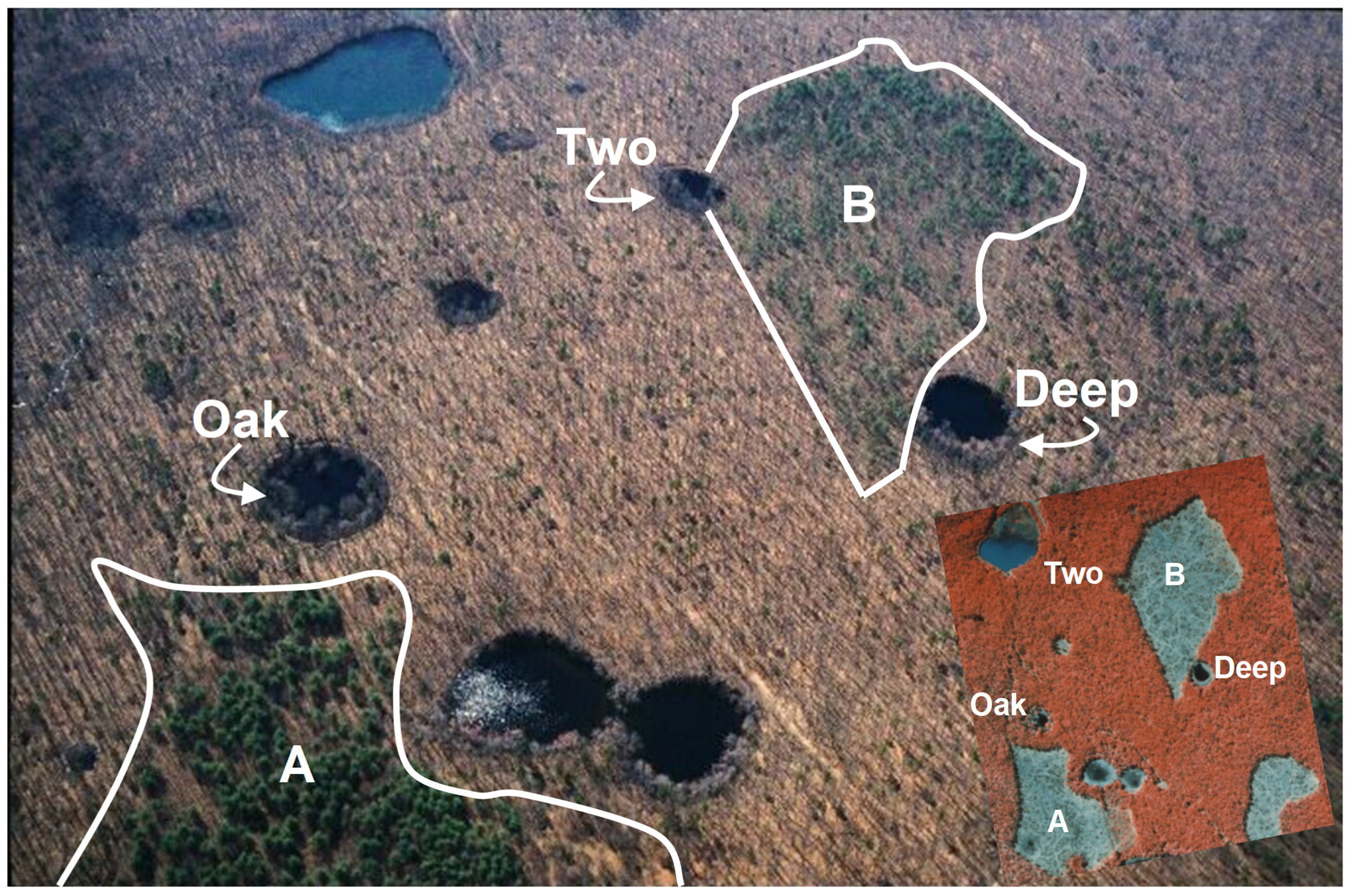
2.1. Study System and Field Methods

Our study focuses on Ambystoma opacum populations associated with three geographically isolated breeding ponds (Pond Two, Oak Pond, and Deep Pond) in the Maple Flats Sinkhole Pond Complex [22] at the base of the Blue Ridge Mountains in the Shenandoah Valley of Augusta County, VA, USA. Our study ponds are within the Big Levels Wildlife Management Area of the United States Forest Service’s Pedlar District in the George Washington and Jefferson National Forest. Terrestrial stages of Ambystoma opacum are largely subterranean in upland forests; typically, adults breed explosively after heavy rains from late August through September. During a dry fall, breeding migrations at our study site eventually occurred in smaller numbers during rainless nights by October. Mating occurs in and around dry pond basins, and females deposit their clutch under cover before ponds fill. Females often remain with the eggs until the site floods, usually through early November, and may not exit the pond basin until the following spring when ponds fill late in the season (D. R. Church, unpublished data). Little is known about the terrestrial ecology of this species. Juveniles return to breed 1–6 years following metamorphosis [23]; in our system, juveniles began recruiting into breeding populations at age two (Church, Bailey, and Wilbur, unpublished data). In continuous, mature forest habitats, adult breeders exhibit high site fidelity with a maximum dispersal distance of 493 m (>95%; [24]). Surviving males tend to breed each year, but female breeders may skip breeding opportunities [25].
Our focal study ponds are arranged in an approximately equilateral triangle (325–400 m apart). Each pond is associated with a clearcut that was harvested in 1980 (Figure 1) and is otherwise surrounded by a mature forest habitat that was extensively coppiced for fuelwood in the 1800s, but has not been cut since the early 1900s. Church (2008) reports other ponds in the Maple Flats complex that support A. opacum, but only Twin Ponds are within 200 m of the focal study ponds [26]. The mature forest stands are dominated by hardwoods including oak (Quercus rubra, Q. prinus, Q. alba, and Q. concinnea), hickory (primarily Carya glabra and C. tomentosa), black gum (Nyssa sylvatica), and yellow-poplar (Liriodendron tulipifera) interspersed with an occasional pitch or shortleaf pine (Pinus rigida and Pinus echinata, respectively). The clearcuts were partially replanted with white pine (Pinus strobus) at higher densities than pines occur in the surrounding forest. At the onset of our study in 1999, 19 years post-clearcutting, stem size and abundance of trees were still different between regenerating clearcut and mature forest habitats surrounding each of our study ponds (H. M. Wilbur and D. R. Church, unpublished data).
Each pond was completely encircled by a drift fence buried 10 cm below the surface and pitfall traps 19 L in size buried flush with the ground surface at 10 m intervals on both sides of the fence in the summer of 1999, prior to the onset of the Ambystoma opacum breeding season. Pitfalls were checked daily and throughout the night during peak amphibian migrations. Pitfalls were only closed during freezing weather or on some days during drought conditions outside of the seasons for amphibian breeding and metamorphosis, when no animal movements were occurring. Oak and Deep Ponds had 290 m drift fence perimeters, with 70 m and 140 m, respectively, associated with regenerating clearcuts (Figure 1). An approximately 30 m forest buffer was left between the clearcut and Oak Pond to protect its wetland plant community. Pond Two, with a 210 m total drift fence perimeter, had 70 m of the perimeter associated with regenerating clearcut (Figure 1).

2.2. Reconstructing Individual Capture Histories

Using the drift fences and pitfall traps, Ambystoma opacum were captured entering and exiting the study ponds in four consecutive years, including the 1999–2000 breeding season through the 2002–2003 breeding season. Captured animals were photographed to identify individuals via natural dorsal markings (Figure 2). Our dataset includes 32,843 captures representing 11,718 individuals. A pattern matching software designed specifically for Ambystoma opacum by one of the authors (LH, see https://conservationresearch.org.uk/Home/ExtractCompare/salamander.html accessed on 18 April 2022) was used to aid in the construction of capture histories. To reduce the risk of misidentification, four body sections from each image were extracted separately and compared to the complete library of images. The four body sections included: the head pattern only, a section of body from the front limb insertions to the animal’s midpoint; a section from the midpoint to the hind limb insertions, and the animal’s entire dorsal pattern from the head to the hind limb insertions (i.e., excluding only the tail pattern). For each section extraction, the program ranked the images in the library according to their likelihood of being a match. One person (JHG) visually examined the top 10 ranked images for each of the four section extractions and made a determination as to whether or not the animal in the photograph had been previously captured. To test the matching process, we introduced a set of photos for 500 known individuals using two different body postures (i.e., 1000 test photos representing 500 individuals) to test the accuracy of the matching software. We recorded the proportion of images where the true match appeared in the top 10 ranked images.
Metamorphs and post-metamorphic juveniles were also captured and recorded but were not included in the multistate mark-recapture analysis until they returned to breed for the first time as adults because their patterns do not fully develop until they reach maturity. Captures of post-metamorphic juveniles were extremely rare (<5 total captures) because they remain in the upland forest habitat until they mature at age 2 years or older (Church, Bailey, and Wilbur, unpublished data).

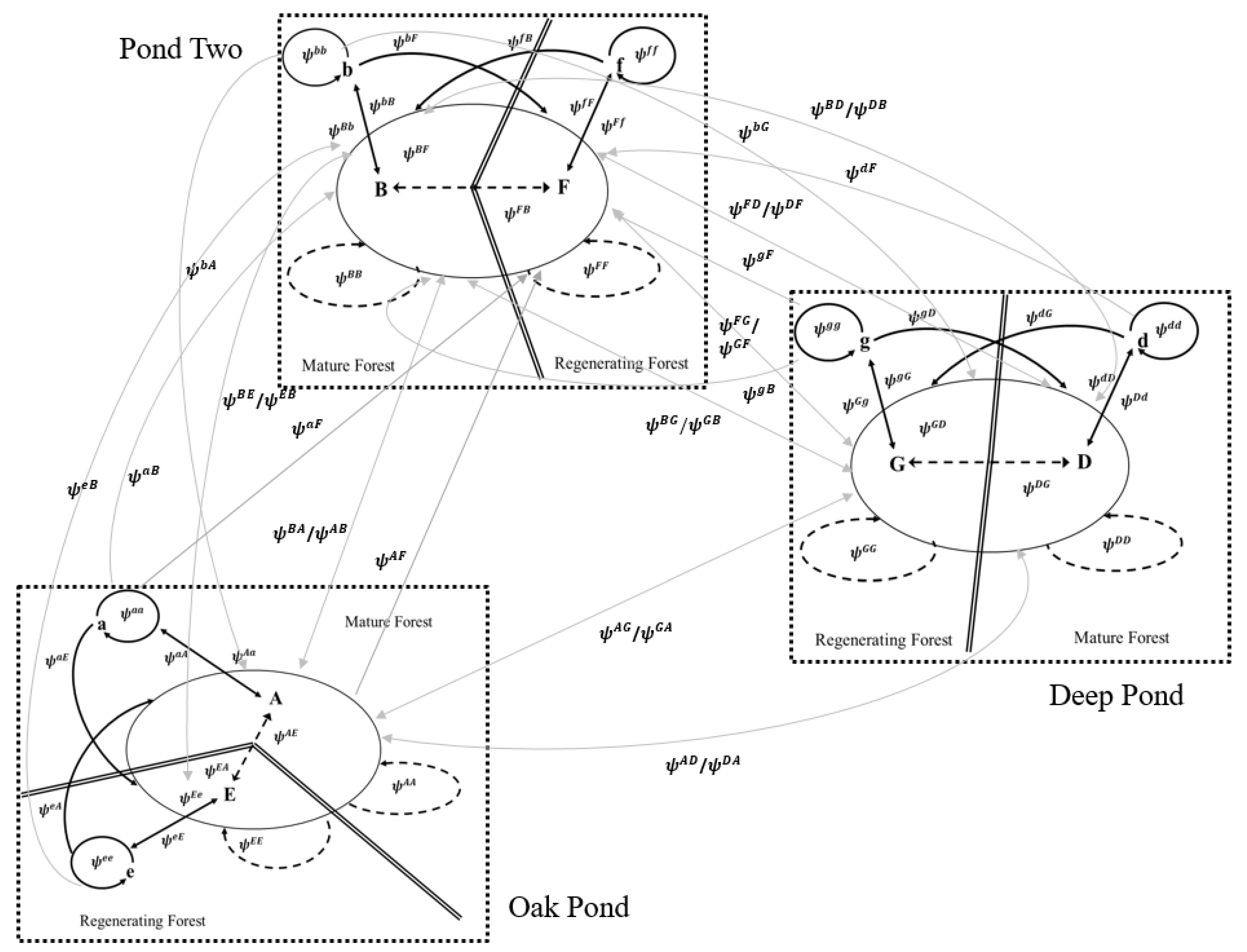
2.3. Multistate Mark-Recapture Analysis and Multimodel Inference

We used multistate mark-recapture models (MSMR) to estimate survival, movement, and breeding probabilities for salamanders associated with regenerating clearcut or mature forests at each geographically isolated breeding ponds [27,28,29]. Specifically, each pond (population) included four states, denoting whether individuals were breeders or non-breeders in a given habitat type (regenerating or mature forests; Figure 3). The entire study system was represented by 12 states and transitions include switching between breeding and nonbreeding states at a given pond (breeding probability) and movements between regenerating and mature forests at a given pond (local movement) or between ponds (landscape movement). This modified robust design model [27,28,30] permits breeders to move between habitats during the breeding season (i.e., within a primary period) by entering the pond basin from one habitat (e.g., regenerating forest) and leaving into another habitat (e.g., mature forest). Movements among all observable (breeders) states and transitions between breeding and nonbreeding states (i.e., skipped breeding) are estimated between breeding seasons (primary periods; Figure 3). Transitions between two nonbreeding states are not estimable and are assumed to be zero [28,29].
Survival probabilities estimated for breeding (observable) individuals are assumed to be equal to those for non-breeding (unobservable) individuals; this is a common assumption for MSMR systems with unobservable states (i.e., that unobservable nonbreeders, U, and observable breeders, O, have equivalent survival probabilities: S t U = S t O , see [30] and citations within). Another fundamental assumption of all MSMR models is that the state-specific survival probability from occasion t to t + 1, S t s t , is a function of the individual state at time t. For example, a breeder that exits the pond into the regenerating forest is assumed to survive in the regenerating forest during the subsequent non-breeding season. This state-specific survival assumption is common in MSMR studies [29,30]. We verified that all parameters in the models described below were identifiable using two numeric methods (see [28,29] for method details).

2.4. Candidate Model Set and Model Selection

We fit a series of models to test our a priori hypotheses about potential differences in salamander survival and breeding probabilities between regenerating and mature forests and movements among multiple geographically isolated wetlands surrounded by heterogeneous forest types. We analyzed data for males and females separately because the relative lengths of primary periods differed between the sexes, as the time spent within the pond basin was usually longer for female breeders (Appendix B). Our global model, denoted S(t×hab×pond) ψ (br_hab×pond, loc_hab×pond, land_hab×pond) p(ct), allows survival probabilities (S) to differ among the breeding and non-breeding seasons of all four years (t), between regenerating and mature forest habitats (hab), and among all three ponds (pond). Transition probabilities (ψ) include both breeding (br) and movement probabilities and varied among habitats and ponds. Local movements (loc) occur between habitats associated with a single population (e.g., ψOak,RF-Oak,MF or ψOak,MF-Oak,RF), where RF and MF denote regenerating and mature forest habitats, respectively. Landscape movements (land) occur between ponds and can involve switching habitats (e.g., ψDeep,RF-Oak,MF) or remaining in the same type of habitat (e.g., ψOak,MF-Two,MF). Finally, we used our knowledge of sampling effort to model capture probability, p, across time (occasions). On two occasions, not all captured animals were photographed. During the first occasion in September 1999, we released animals exiting the ponds because we were not yet prepared to safely process the large number of captured animals. The second event occurred on a single night in November 2000, when approximately 70% of the animals exiting the ponds were released without photographs because a forecasted cold front would have reduced the ability of animals to seek cover in the upland habitats. We developed a capture probability structure, denoted p(ct), that assumed capture probability was unique for each pond and habitat, but constant among all occasions, except the two mentioned above.
Starting with this global model, we developed a series of reduced model structures for each parameter type designed to directly test our two hypotheses (see Appendix B for complete list of candidate models). Specifically, we considered four survival structures where survival probabilities: (1) only differed among the breeding and non-breeding seasons of all four years (S(t)), (2) differed by all seasons and ponds (S(t×pond)), (3) differed by all seasons between regenerating and mature forest habitats (S(t×hab)), and (4) difference by seasons, ponds, and habitats (S(t×hab×pond). We considered seven transition probability structures, including three where breeding and local movements varied between habitats and ponds (br_hab×pond, loc_hab×pond) and landscape movements either varied by habitat only (land_hab), by habitat and pond (land_hab×pond), or was constant (denoted by no land label). We also considered transition probability structures where all breeding and movement probabilities varied among habitats (br_hab, loc_hab, land_hab) or were constant (.), and structures where breeding and local movement probabilities varied with either habitat or pond and landscape movements were constant (Appendix B). Finally, we constructed models using the aforementioned capture probability structure, p(ct), and a full time-varying structure where capture probabilities varied among sampling occasions, ponds, and habitats, denoted p(t*) for simplicity. We constrained only the last capture probabilities p(t) = p(t − 1) for each pond and habitat combination, to avoid confounding among parameters at the end of the time series [27,29,30].
We fit all combinations of our four survival, seven transition probability, and two capture probability structures (56 models) to capture–recapture data for males and females separately using the MSMR model in program MARK [31]. A universal goodness-of-fit test for complex MSMR models with unobservable states does not currently exist. We used the most general available procedure, the median ĉ approach implemented in Program MARK, to estimate overdispersion and adjust model selection criteria. Specifically, we used Akaike’s Information Criterion corrected for overdispersion (QAIC) and associated model weights (wi) to evaluate our competing hypotheses.

3. Results

Over our 4-year study, we captured over 15,000 salamanders entering the pond basin; counts were approximately 3.5 times higher at pitfall traps along the perimeter of mature forests habitat (Appendix A, Table S1). Count ratios (mature:regenerating forest) exceeded expectations based on relative perimeter lengths for each forest type at two of the three ponds for both male and female salamanders (Appendix A).

3.1. Matching Individual Capture Histories

Using photos from two body postures on the subset of 500 known individuals, there was a 0.96 probability that the true, known matching photo of the same individual occurred in the top ten library ranking and was selected for at least one of the image extractions. On average, the probability of making successful matches was higher than 0.96 in our study given that a captured individual could be represented by more than one image in the library (i.e., could have been captured multiple times).

3.2. Overall Inference and Model Selection Results

We found little evidence for our first hypothesis that survival and breeding probabilities were reduced in the regenerating forest habitat. We found no evidence that apparent survival probabilities differed between regenerating and mature forest habitats for either sex. Additionally, our expectation that breeding probabilities would be higher for individuals in the mature forests was only supported at one pond (Oak Pond). We did find that former clearcuts influenced local movement probabilities within the basin, as breeders favored mature forest habitats at two ponds (Oak Pond and Pond Two). However, we found no differences in movement probabilities between forest types that occurred in the upland habitat, except for Pond Two; i.e., no differences in local and landscape movements during the nonbreeding season.
Model selection results suggested that all demographic parameters varied among geographically isolated wetlands (ponds). For males, a single model S(t×pond) ψ (br_hab×pond, loc_hab×pond, land_hab×pond) p(t*) represented the data better than any other in the candidate set (w = 1.0; Table 1, Appendix B). For females, three models garnered the majority of the weight of evidence (over 99%, Table 1, Appendix B): these models differed primarily in their survival structure. Survival probabilities varied among years for both sexes, declining dramatically during drought conditions in 2001–2002. We found some evidence of overdispersion and used estimated ĉ = 1.49 for males and ĉ = 1.58 for females to adjust Akaike’s Information Criterion (QAIC) and measures of precision. Detailed results for each demographic parameter are given in the following subsections.

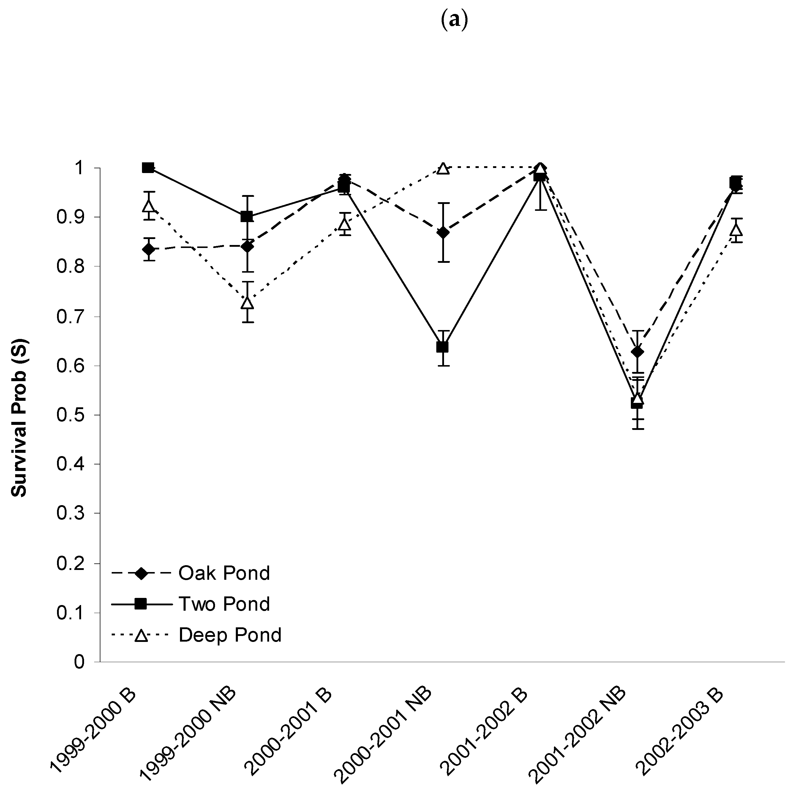
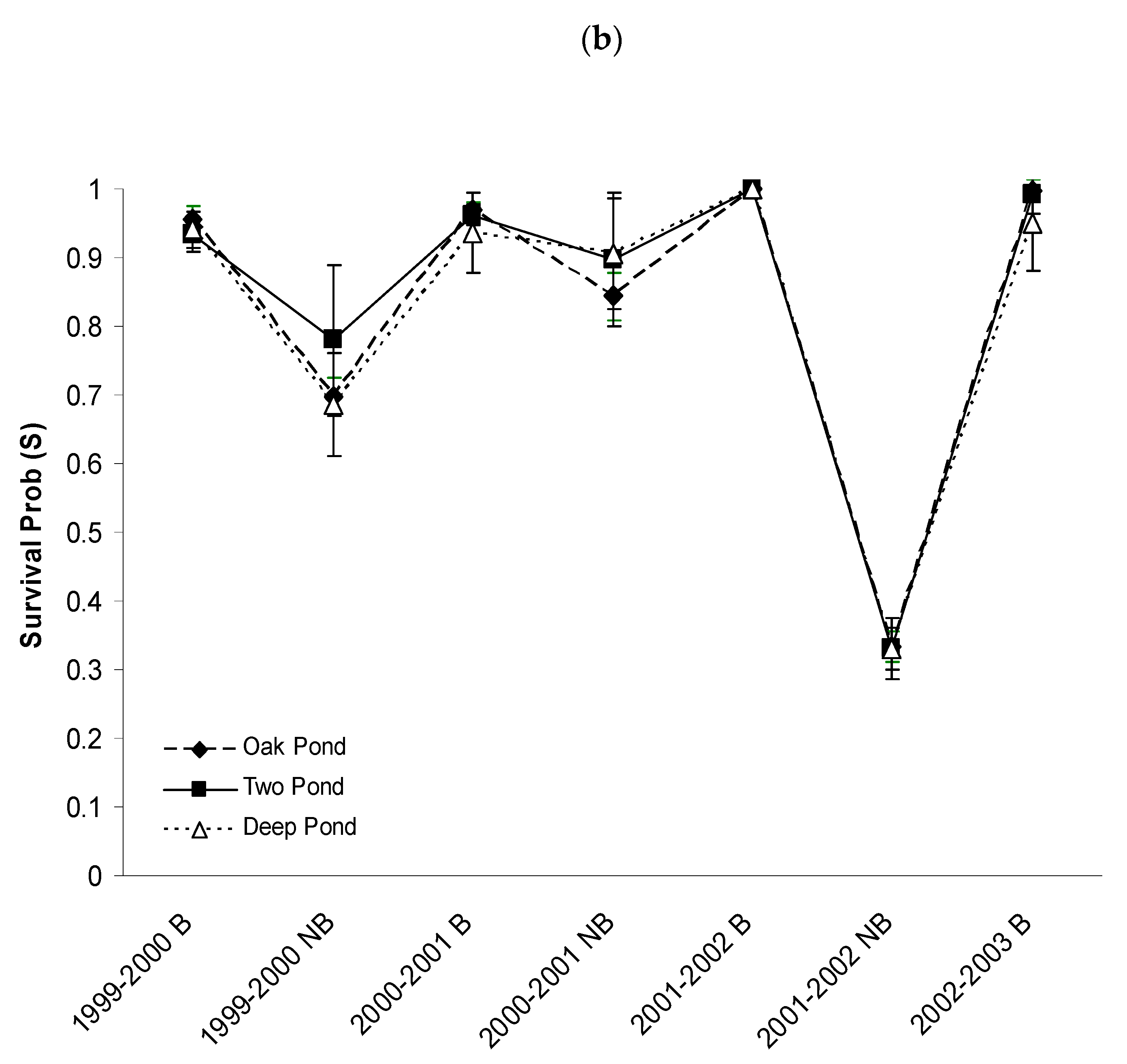
3.3. Apparent Survival Probabilities

While there was little evidence that survival probabilities varied among habitats, there was strong evidence that survival probabilities varied among the three ponds for males, and to a lesser degree for the females. We present realized survival probabilities that reflect survival probabilities over time periods that correspond to breeding and non-breeding seasons in each year. It is important to note that these time intervals differed among years, ponds (populations), and between females and males. For example, males typically spent an average of 20–35 days within the pond basins during the breeding season, whereas females typically spent 45–65 days in the pond basin (Appendix A).
Male survival probabilities during the 3–4 week breeding season were fairly high and stable across years and ponds, ranging from 0.87–1.0 (Figure 4a, Appendix C). Male survival during the longer (~11 month) nonbreeding season varied among ponds and years, ranging from 0.52 and 1.0 (Figure 4a, Appendix C). Survival results were similar for females, with slightly more consistency among ponds (Figure 4b, Appendix C). Model-averaged survival probabilities for females ranged between 0.92 and 1.00 during the ~2 months females were in the pond basin (breeding season) and from 0.33 to 0.91 during the non-breeding season (Figure 4b, Appendix C). All populations were affected by the extremely dry 2001–2002 year, where the lowest survival probability estimates for both sexes occurred in the non-breeding season during that year (Figure 4). Although we did not formally test for sex-specific differences, female survival probabilities dropped to 0.33 (SE ≤ 0.04) in all populations, but male survival probabilities remained above 0.52 (SE = 0.05, Pond Two, Figure 4).

3.4. Breeding Probabilities

Model selection revealed that breeding probabilities varied between habitats and ponds for both females and males (Table 1, Figure 5, Appendix B). Estimates of breeding probabilities revealed: (1) sex-specific differences in breeding frequency and (2) a range of findings across ponds with respect to effects of habitat type. Males are more likely to breed in successive years than females, while females that skipped breeding (NB) had a much higher probability of breeding the following year than successive female breeders (Figure 5). For example, the probability of breeding for females at Oak Pond is lower for individuals that breed the previous year (0.37 (SE = 0.06) and 0.52 (SE = 0.02), for regenerating and mature forest habitats, respectively) compared to individuals that ‘skipped’ breeding opportunities for one or more years (0.71 (SE = 0.15) and 0.86 (SE = 0.05), for regenerating and mature forest habitats, respectively: see Figure 5b). Breeding probabilities were slightly higher for both sexes for individuals exiting into the mature forest at Oak Pond, similar among habitats at Pond Two, and slightly higher for individuals exiting into the regenerating forest at Deep Pond (Figure 5).

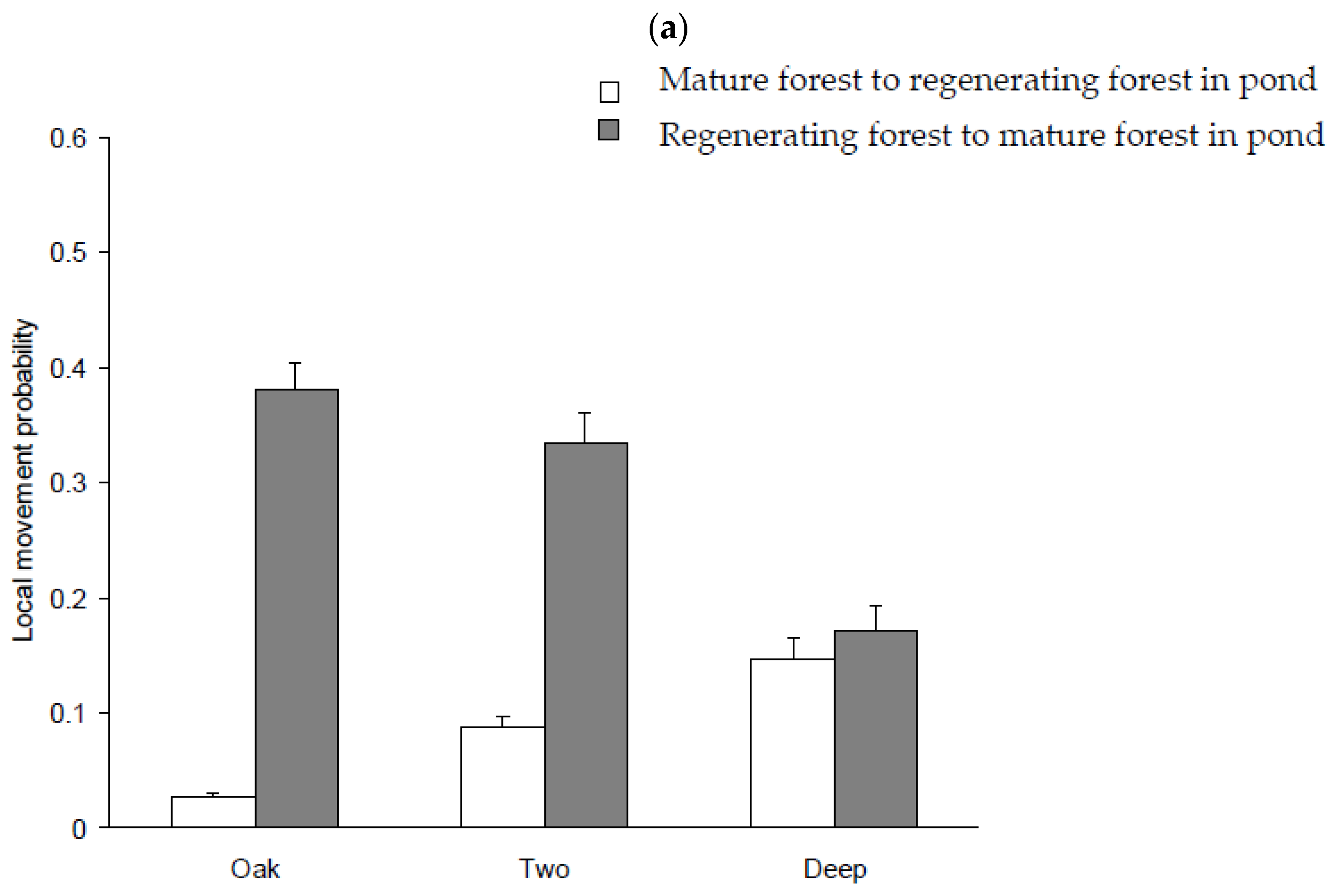
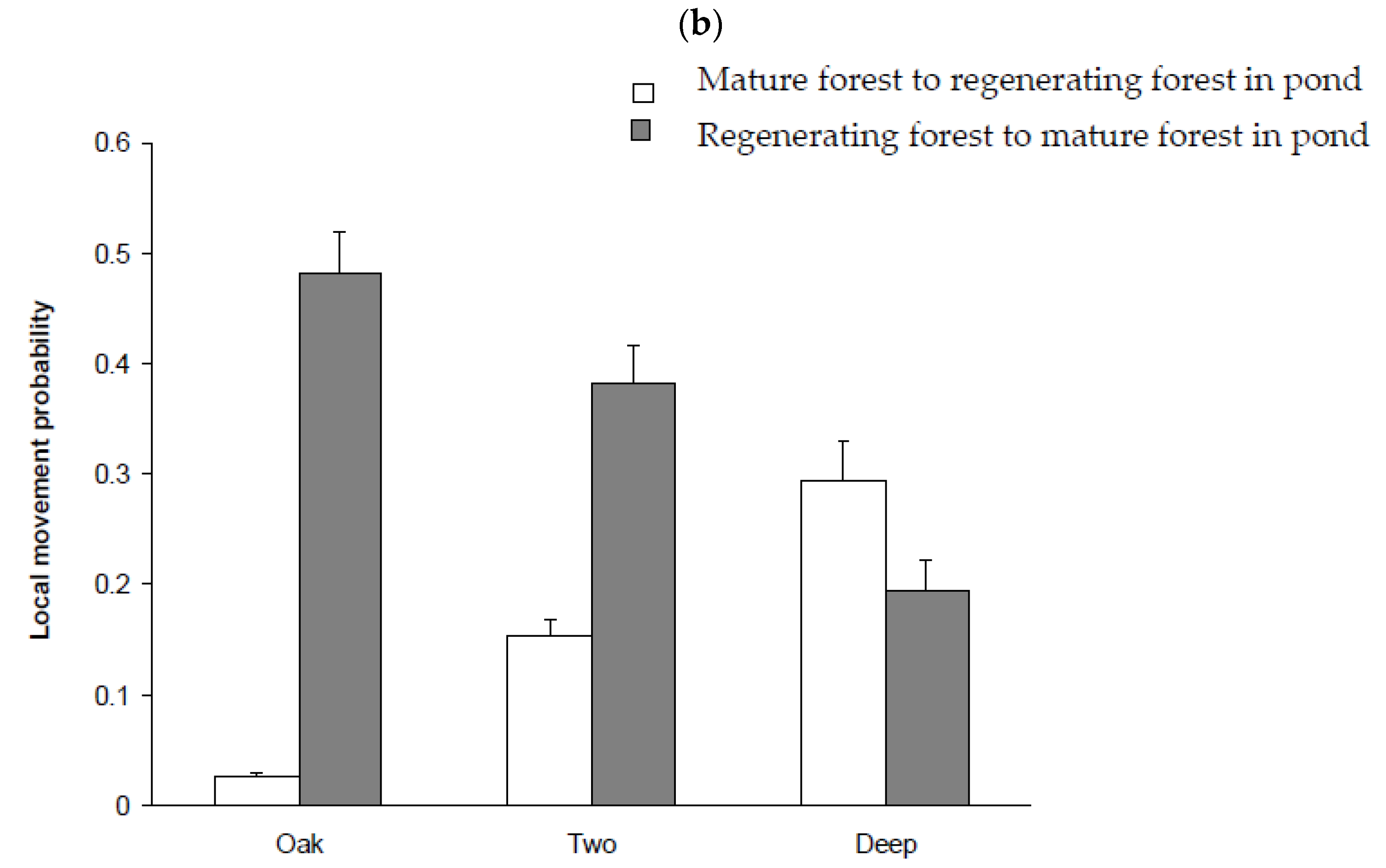
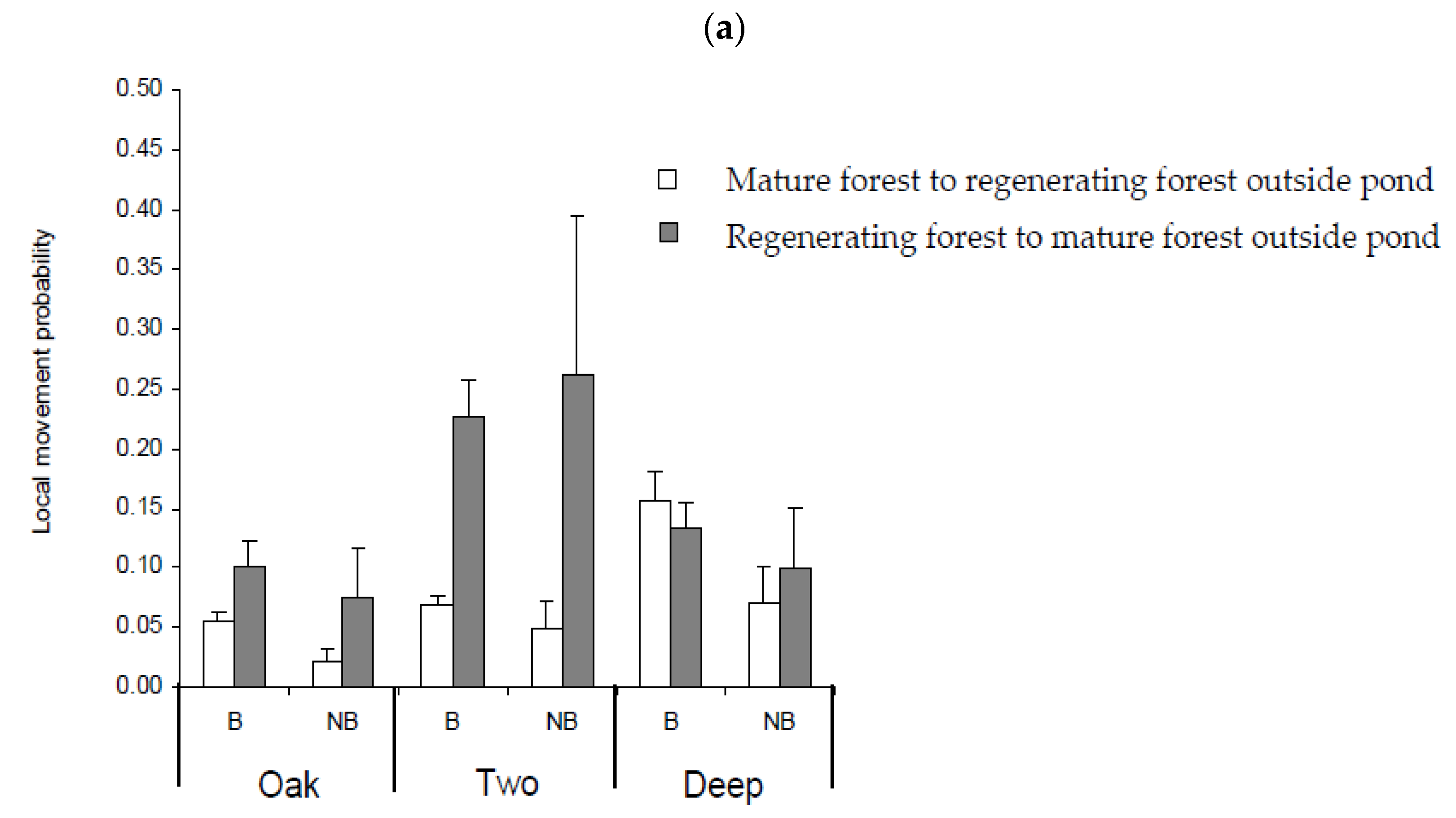
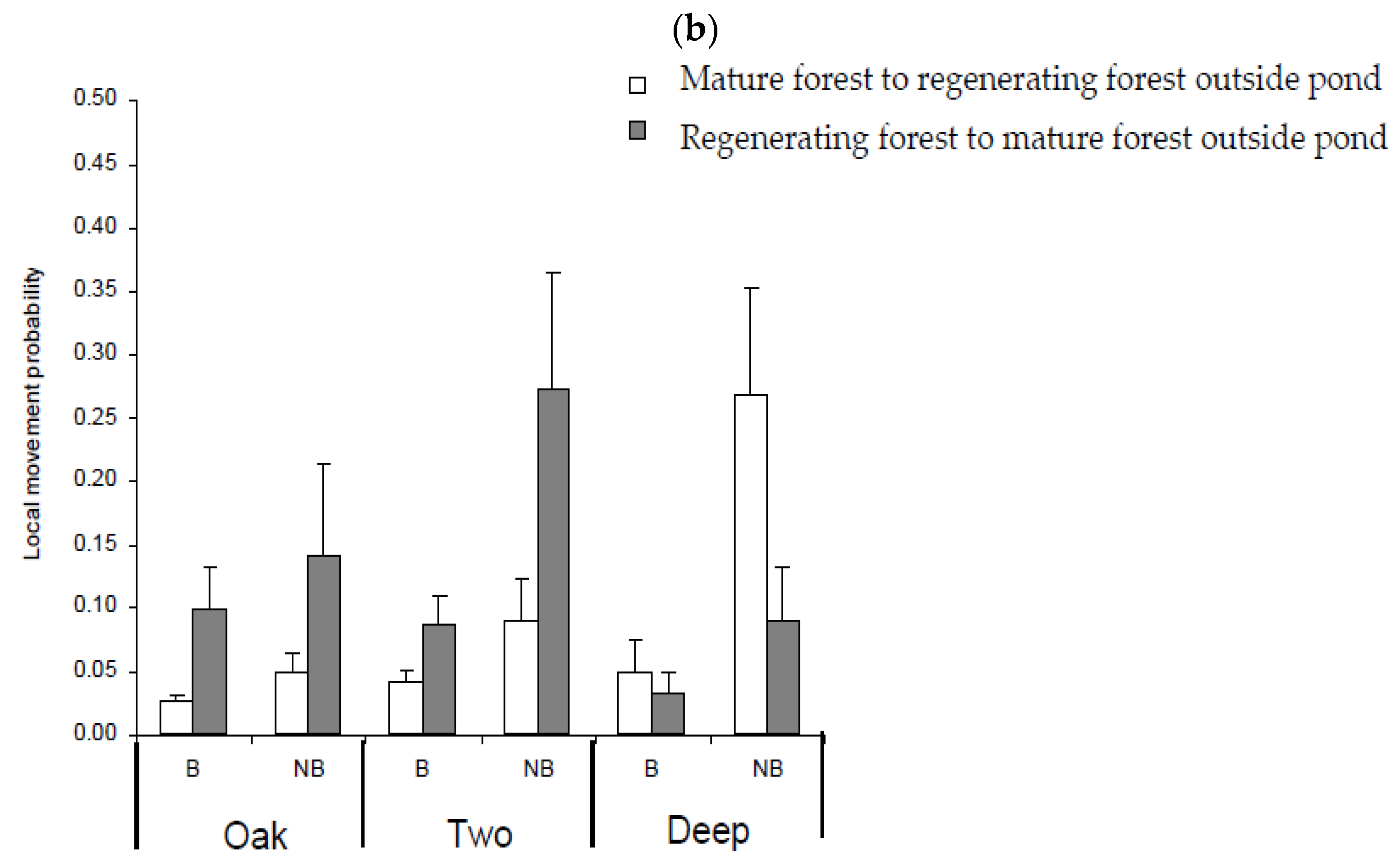
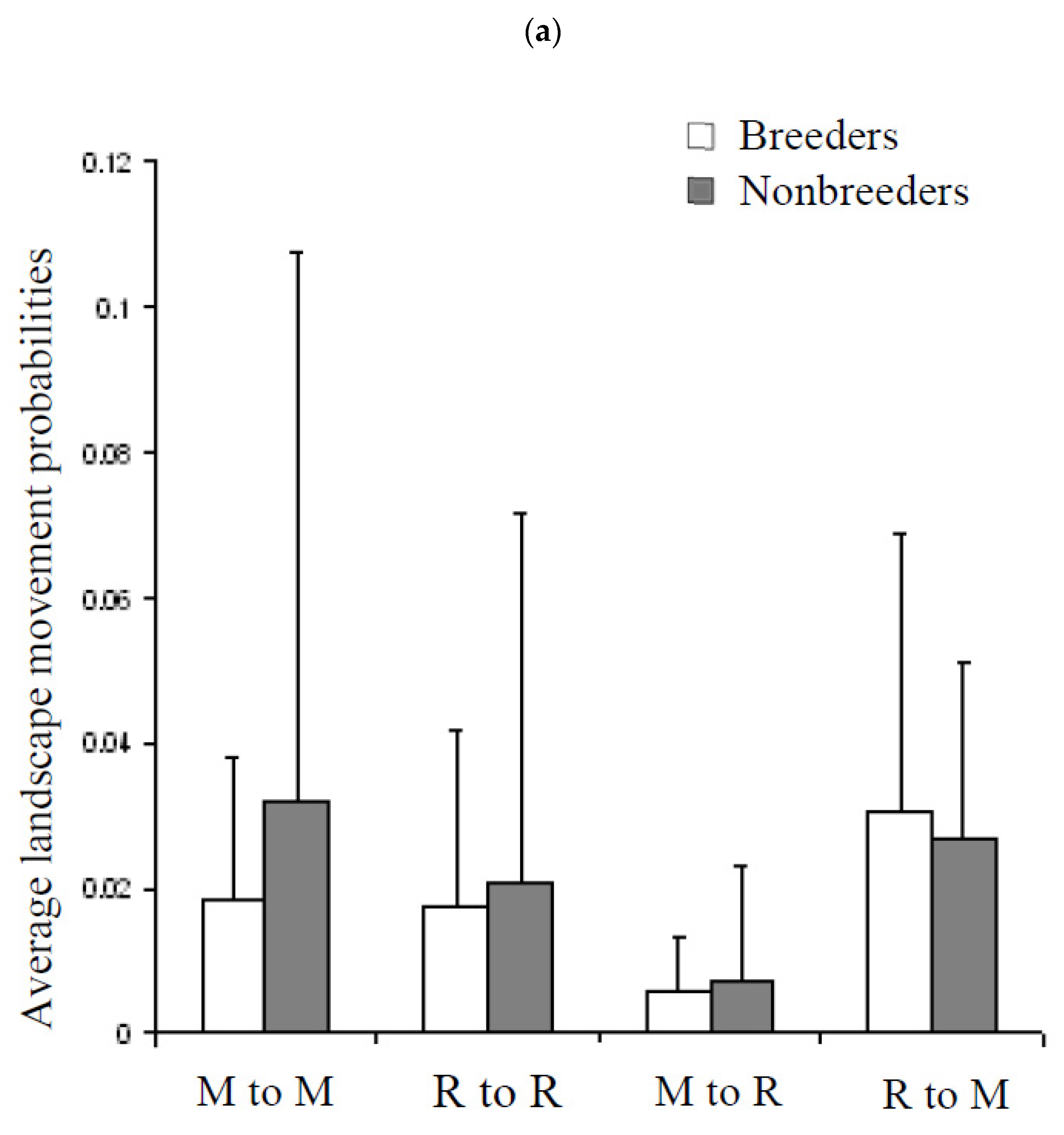
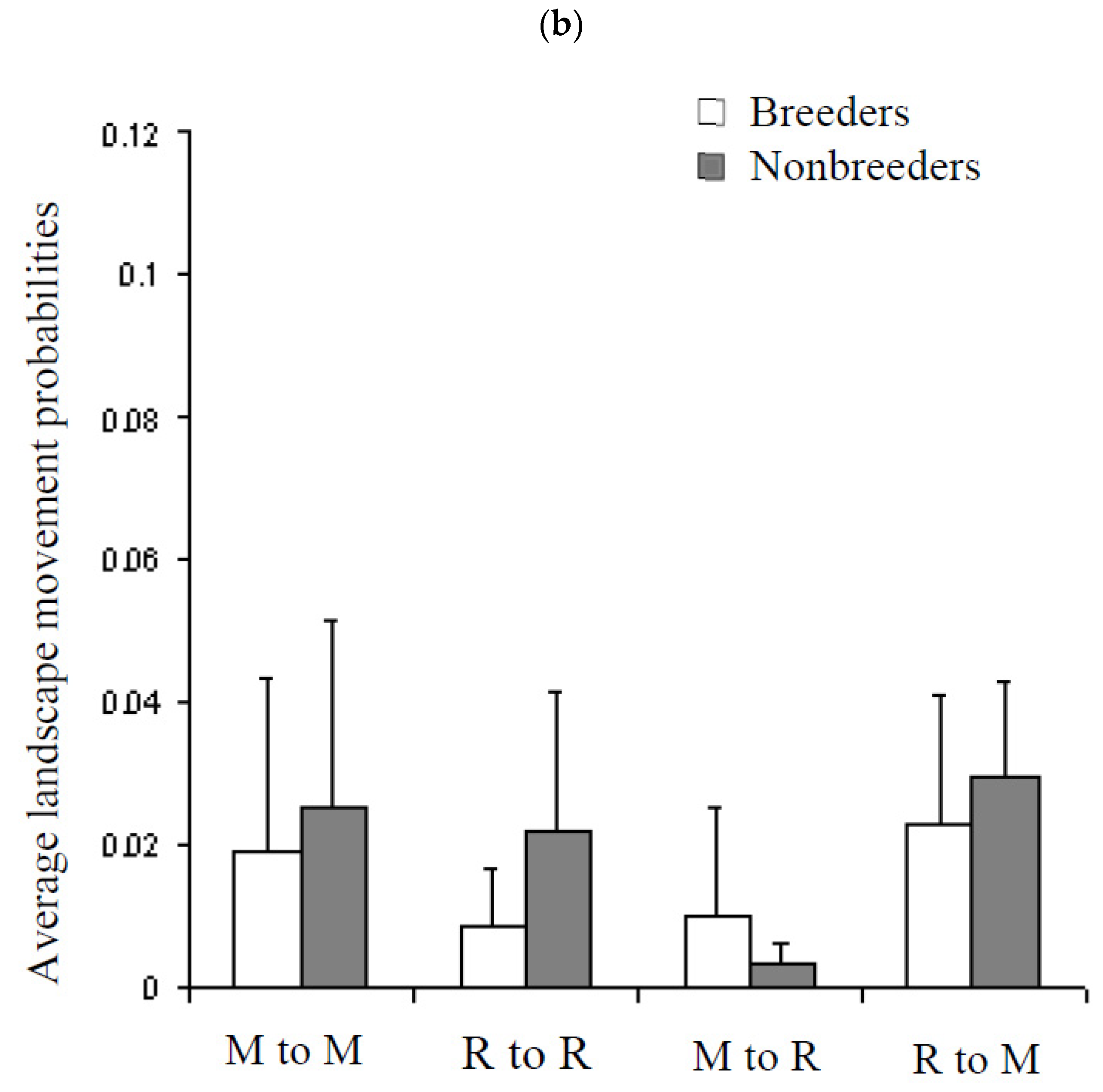
3.5. Movement Probabilities: Local and Landscape

We found support for the hypothesis that salamanders selected mature forest locally, especially breeders exiting the pond basin. Local movement probabilities within the pond basin during the breeding season were relatively high and varied among ponds (Figure 6) but indicated that both sexes preferentially moved from regenerating to mature forest habitats at two ponds (Oak Pond and Pond Two; Figure 6). This trend was not apparent within Deep Pond where it appears that the exchange between local habitats was approximately equal (males) or actually favored the regenerating forest habitat (females). Local movements between upland habitats during the non-breeding season were generally lower but exhibited similar trends (Figure 7, Appendix D). Again, movement probabilities associated with populations at Oak Pond and Pond Two were consistent with our a priori expectations for movement probabilities, but movement probabilities at Deep Pond were not.
Inferring that salamanders actively avoid formerly clearcut habitat in favor of more mature forest requires that local movement probabilities differ from simple random movements. Conservatively, if animals enter and exit the pond basin at random, we would expect their movement probabilities to be proportional to the available habitat. Thus, we might expect there to be higher movement probabilities from regenerating to mature forest habitats at Oak Pond and Pond Two simply based on the proportion of available habitat (mature: regenerating forest ratios around pond perimeters were 3:1 at Oak Pond, 2:1 at Pond Two, and 1:1 at Deep Pond; Appendix A). However, ratios of male movement probabilities from regenerating to mature forest habitats within the pond basins were approximately 13:1 for Oak Pond, 3.5:1 for Pond Two and 1:1 for Deep Pond (Figure 6a). Similarly, ratios of female movement probabilities from regenerating to mature forest habitats within the pond basins were approximately 16:1 for Oak Pond and 2.5:1 for Pond Two but were higher from mature to regenerating forests at Deep Pond (Figure 6b). Local movement probabilities within the pond basis suggest that salamanders favor mature forested habitats in 2 of the 3 study ponds.
Landscape movement probabilities involving movements between ponds were generally lower than local movements: most were ≤0.05 (Appendix D). Means of landscape movement probabilities between ponds tended to be remarkably similar regardless of habitat types, but landscape movements involving transitions from mature to regenerating forests were exceedingly rare (Figure 8, Appendix D).

3.6. Capture Probabilities

Capture probabilities were usually high, except for the occasions when not all trapped individuals could be photographed (Appendix E). Probabilities for males ranged from 0.20 to 0.99 and between 0.28 and 1.00 for females (Appendix E). Our large sample sizes and high capture probabilities resulted in precise survival estimates.

4. Discussion

Numerous studies have investigated how amphibians respond to immediate alterations of forest habitat (e.g., [11,16,17,32]), but few have explored the lasting effects of clearcuts on amphibian demography [18]. Our study explored hypotheses as to why fewer individuals of Ambystoma opacum were observed migrating to breeding ponds from 20-year-old regenerating forest than from mature forest stands (Appendix A). We used MSMR models with unobservable states to specifically test two hypotheses: (1) that animals have lower survival and breeding probability within 20-year-old regenerating forests, and (2) that movements of animals at local and landscape scales preferentially favor mature forest stands (i.e., that salamanders exhibited informed movements toward more favorable habitat). Overall, we found some support that local movements within pond basins by both sexes favor mature forest habitats; however, the variation in demographic parameters among habitats and ponds indicates that salamander demography and forest structure remain dynamic after 20 years of forest reestablishment and may well be influenced by other environmental factors that were not studied.

4.1. Factors Influencing Survival Probabilities

Although we predicted that survival probabilities would be lower in regenerating forests, our results revealed that survival probabilities did not differ between regenerating and mature forests but did differ among years and ponds (especially for males). It should be noted that survival during the breeding season represents ‘true’ survival, as movement to other populations does not occur while an individual is within a pond basin. Survival probabilities during the non-breeding season should be considered ‘apparent’ survival probabilities reflecting the probability that an individual survives and remains within the 3-pond study system. Still, we believe that permanent emigration to other breeding ponds is low. There was only one set of ponds within 200 m of our focal ponds and previous studies [24] and our results suggest that surviving adults have high site fidelity (typically ≥90%). Studies examining the early effects of clearcuts on amphibians have found that survival can be depressed initially due to microhabitat conditions and desiccation risk [11,33,34], but that this may not always be the case [35]. Rothermel and Luhring (2005) found that the availability of burrows could mediate mortality risks in Ambystoma talpoideum due to dehydration in recent clearcuts [19]. Our anecdotal observations of high small mammal abundance in pitfall traps within the clearcuts we studied suggest that burrow availability is probably substantial after 20 years of forest reestablishment.
Our study overlapped with one of the driest years on record (2001–2002), thereby providing an opportunity to test how regenerating clearcuts may affect salamanders under especially harsh environmental conditions. Our results suggest that drought conditions severely reduce salamander survival probabilities at all three ponds, but we found little evidence that the effect differed between regenerating and mature forest habitats. Relative to breeding seasons in other years, neither sex suffered especially high mortality within ponds during the drought year; however, during the subsequent non-breeding season, survival probabilities at all three ponds fell to their lowest point and were especially low for females, hovering around 0.30 for all populations. We conclude that drought conditions have a major impact on Ambystoma opacum survival even when these animals have an opportunity to seek shelter in the upland habitats. Increasing frequency of dry years has been linked to amphibian population declines in other amphibian species in the southeastern USA [36]. However, Daszak et al., (2005) discussed declines in the context of recruitment failure and not the effect of dry conditions on adult survival [36]. Our findings together with Church et al.’s (2007) estimates of high mortality in a syntopic congener, Ambystoma tigrinum, suggest that the impact of dry conditions on adult survival may also contribute significantly to population dynamics [37]. Indeed, population modeling of amphibian life cycles reveal that population growth tends to be more sensitive to perturbations in survival of terrestrial life stages than to fluctuations in breeding success [14,38,39,40,41]. Climate-related variation in adult survival probabilities has rarely been explored in amphibian populations (but see [13,42] for a review), but its effects and contribution to population declines in some species should be more rigorously investigated [43]. Our findings of simultaneous survival declines among all populations suggests that drought, or climate, are likely primary drivers of both local and spatially-structured population dynamics.

4.2. Factors Influencing Breeding Probabilities

Among potential lasting impacts of clearcutting on demographic parameters, the effects on female breeding probabilities are expected to influence local population dynamics more than the local or landscape movements discussed below. Whereas the local movements may contribute substantially to the differences in abundances of animals residing within the respective upland habitats, these behaviors do not reduce the size of the local or spatially-structured populations of organisms within the broader landscape.
We found that breeding probabilities varied between male and female salamanders and that the influence of habitat on breeding probability differed among ponds. Similar to other studies, we found support that females are less likely to breed in successive years than males. Previous work in the same study system overwhelmingly supported Markovian breeding probabilities for females of two other species, Ambystoma tigrinum [37] and Ambystoma maculatum (D. R. Church, H. M. Wilbur, and L. L. Bailey, unpublished data) and this same breeding pattern has been documented in other A. opacum studies [25] and other pond-breeding amphibians (e.g., [44]).
Breeding probabilities were lower for female breeders exiting the pond into regenerating forest habitat at two of the three ponds (Oak Pond and Pond Two; Figure 4b). However, the habitat effect was only apparent at one of these ponds (Oak Pond) if females skipped one or more breeding opportunities (i.e., for nonbreeders). We do not know why females that exit the pond into regenerating forests near Oak Pond and Pond Two are less likely to breed in consecutive years, but we infer that females in these populations can assimilate resources for breeding more efficiently within mature forest habitats (but see [35]). For example, the planted pines in the regenerating forest may change leaf litter composition and the terrestrial invertebrate prey abundance [45]. Furthermore, because there was a minimal effect of habitat type on the breeding probability of nonbreeding females near Pond Two, we suggest that the resources for reproduction may be assimilated at different rates among different regenerating forests.
Contrary to expectations, breeding probabilities for all salamanders associated with Deep Pond had slightly higher breeding probabilities for individuals exiting into the regenerating forest (Figure 4). One possible explanation is that other important environmental factors vary between the regenerating and mature forests at Deep Pond, emphasizing that lasting impacts of clearcuts may vary among geographically isolated wetlands within the same landscape.

4.3. Factors Influencing Local and Landscape Movements

Local movements of adult breeding salamanders at Oak Pond and Pond Two indicate a propensity to leave regenerating forest and remain in mature forest habitats. Similar movement preferences were seen outside the pond basin, during the nonbreeding season, for individuals at Pond Two (Figure 6). These movement preferences for mature forest habitat exceed random expectation based on relative amounts of regenerating and mature forest surrounding each of the ponds. Previous studies of ambystomatid salamanders show that emigration paths from ponds are typically straight and perpendicular to the pond’s edge [21,46,47,48]. Other studies have shown that amphibians tend to navigate based on immediate cues and have limited abilities to perceive, orient, and navigate based on distant cues [49,50,51]. Collectively, these studies would suggest that in unmanipulated habitats individuals are likely to exhibit a high degree of fidelity to entry and exit points, but individuals near the edge/intersection of habitats are more likely to perceive and orient based on habitat differences. In recent timber harvests, salamanders exhibited the highest movement out of clearcut habitats [17] and the greatest affinity for remaining forested habitats of all amphibians [52]. Individual salamanders in our study populations had a high degree of fidelity to their entry and exit locations within and across years, exiting ponds within 20° of their entry point (as measured from the ponds’ hydrological centroid) and returning within 25° of their exit point (D. R. Church and H. M. Wilbur, unpublished data). These findings indicate that movements between habitats are made primarily by animals living along the edge of the two habitats, where presumably habitat preference represents a departure from even odds. This alternative expectation for random movement would suggest movement probabilities between habitats should be approximately equal if individuals show no habitat preference. Under this second interpretation, local movement probabilities at Oak Pond and Pond Two (both within and outside the pond basin) certainly appear to favor mature forest habitats, consistent with our a priori predictions. Salamanders at Deep Pond did not differ from our random expectations.
At the landscape scale, movement probabilities between spatially-structured populations (i.e., breeding dispersal) were overall low but highly variable and greater than those for syntopic Ambystoma tigrinum populations [37]. Landscape movements requiring individuals to move from mature forest to or through regenerating forests were rare; these movements had the lowest mean and variance of all landscape movements. Similar informed dispersal has been seen in other spatially-structured populations where individuals favor higher quality habitats [4,53,54]. Moreover, Rittenhouse and Semlitsch (2006) found that adult Ambystoma maculatum avoid crossing grassland habitat and our findings suggest that regenerating clearcuts may have similar negative effects on the probability of colonization if situated between a source and destination pond for dispersing animals [55]. Clearcuts that completely encircle a geographically isolated wetland may increase local extinction risk by reducing a ‘rescue effect’ [56]. However, timber management that maintains a system of corridors among wetlands could permit exchange among populations (i.e., breeding ponds).

4.4. Caveats

Our findings provide new information and methods valuable to the management of pond-breeding salamanders in temperate deciduous forests. However, care should be taken in extrapolating our results to other systems, as parameter estimates are likely to vary among species and populations, as exemplified within our study system. Furthermore, we have not fully answered the question as to why smaller numbers of animals are captured in regenerating forests habitats for two of our focal ponds (Appendix A). It is possible that populations may still be rebounding from mortality incurred during clearcutting activities. Our results indicate that some differences between mature and regenerating habitats persist 20-years post-harvest (e.g., some breeding and movement probabilities), but this does not rule out that initial declines may contribute to reduced animal abundances observed within regenerating forests at two of our study sites (Appendix A). This question is best addressed via a longitudinal study of populations at multiple geographically isolated wetlands, beginning before clearcuts are created and continuing multiple decades post-harvest. The Land-use Effects on Amphibians Project (LEAP), initiated in 2004, is an intensive experimental study of the initial effects of different clearcutting practices on amphibian abundance and demography [17,57]. This project explored initial impacts of clearcutting on resident amphibian populations and has the potential to track how those impacts change over time as the forest regenerates and recovers.
Our study was not a planned experiment, but we capitalized on previous forest management to address our biological questions of interest, despite unequal amounts of previously clearcut habitat around and between each geographically isolated wetland. As with most MSMR analysis we assume state-specific survival, i.e., that survival probability from time t to t + 1 is a function of the individual’s state at time t. We found no evidence that survival probabilities differed between regenerating and mature forest habitats for either sex, but if individuals exited the pond into regenerating forest and simply moved through that habitat and spent the majority of the non-breeding season in mature habitat, we would not detect survival differences relative to individuals that resided entirely within the regenerating habitat. Without a mechanism to track salamanders in the upland habitat, we cannot be certain that an individual’s habitat state at time t reflect the habitat experienced during the interval from t to t + 1. Still, previous studies of ambystomatid salamanders show that emigration paths from ponds are typically straight, relatively short, and perpendicular to the pond’s edge [21,46,48,51] and salamanders tend to have small activity centers in the upland habitat [46,51]. Additionally, we found low movement probabilities between habitat types outside the pond basin, expect for Pond Two, or among geographically isolated wetlands (Figure 6 and Figure 7). Salamanders were much more likely to remain in the same habitat type, suggesting that our state-specific assumption is likely met for most individuals.

5. Conclusions

Our study is one of the few to explore how environmental and habitat factors influence survival, breeding, local movement, and dispersal probabilities for species dependent on geographically isolated wetlands [4,58]. We found that some demographic parameters may rebound following clearcutting (e.g., survival probabilities) but differences exist between mature and regenerating forests two decades post-harvest (e.g., local movements). We suggest that Ambystoma opacum populations can recover from the impacts of clearcutting but that the rate of recovery is probably highly dependent on magnitude and configuration of clearcuts and surrounding mature
We expect that both immediate and lasting effects of clearcutting on demographic parameters may be greater for populations at geographically isolated wetlands that do not have mature habitats in close proximity. In our study system, animals have opportunities to move from regenerating to mature forests and, indeed, appear to do so preferentially, exhibiting informed movement or dispersal, even after 20 years of forest reestablishment. Such local movements may thereby moderate survival of salamanders within landscapes that include regenerating forests. Careful attention should be paid to setting aside tracts of mature forest habitats prior to timber harvest to allow amphibians opportunities to move between habitats to reduce or mitigate for direct losses due to timber harvest. Our findings do indicate that local movements and possibly breeding probabilities are sufficiently different after 20 years to contribute to differences in the numbers of animals in the two habitats.

Supplementary Materials

The following supporting information can be downloaded at: https://www.mdpi.com/article/10.3390/d14050309/s1, Table S1.

Author Contributions

Conceptualization, D.R.C. and H.M.W.; Methodology, D.R.C., H.M.W. and J.H.G.; Software, L.H.; Validation, D.R.C. and J.H.G.; Formal analysis, D.R.C., H.M.W. and L.L.B.; Investigation D.R.C., H.M.W. and L.L.B.; Resources D.R.C. and H.M.W.; Data Curation D.R.C. and J.H.G.; Writing—Original Draft Preparation, D.R.C., H.M.W., L.L.B. and L.H.; Writing—Review & Editing, D.R.C., H.M.W. and L.L.B.; Visualization, D.R.C., H.M.W. and L.L.B.; Supervision, H.M.W.; Project Administration, D.R.C. and H.M.W.; Funding Acquisition, H.M.W. All authors have read and agreed to the published version of the manuscript.

Funding

Funding for this study was provided by the National Science Foundation (DEB 0211985 and DEB 041418 to HMW), U. S. Forest Service, National Fish and Wildlife Foundation, Conservation International, and Sigma Xi Scientific Society to DRC. LLB was also supported in part by USGS Amphibian Research and Monitoring Initiative.

Institutional Review Board Statement

Field methods were approved by the University of Virginia Animal Care and Use Committee and under permit from the Virginia Division of Game and Inland Fisheries and permission of the District Ranger, Pedlar/Glenwood District, George Washington National Forest.

Data Availability Statement

The data presented in this study are available in Supplementary Materials.

Acknowledgments

We thank Fred Huber, Amy Alsfeld, Kurt Buhlmann, Jon W. Church, Sheri A. Church, Mike Donahue, Doug Gant, Dawn Kirk, Joseph Mitchell, Jonathan Richardson, and Greg Ruthig for assistance in the field. We also thank James Nichols, William Kendall, and James Hines for assisting our analysis. We are also grateful to Joseph Van Buskirk, Jr. and two anonymous reviewers for comments on an earlier version of this manuscript.

Conflicts of Interest

The authors declare no conflict of interest.

Appendix A

Raw counts, ratio of counts between mature and regenerating forest, and average (± SD) pond residence times (days) of animals captured entering and exiting each breeding pond basin. Oak Pond had 290 m total drift fence perimeter with 70 m associated with regenerating forest (Figure 1), or approximately 3:1 ratio of mature forest to regenerating forest habitat. Pond Two had 210 m total drift fence perimeter with 70 m associated with regenerating forest (Figure 1), or a 2:1 ratio of mature forest to regenerating forest habitat. Deep Pond had 290 m total drift fence perimeter with 140 m associated with regenerating forest (Figure 1), or approximately 1:1 ratio of mature forest to regenerating forest habitat.
Pond
(Habitat Ratio)
SexYearCount
Mature Forest
Count
Regen. Forest
Count Ratio
Mature: Regen
Residence Time
Oak Pond (3.1:1)Females1999–20006781136.0:161.6 ± 6.0
2000–20017041315.4:163.2 ± 8.1
2001–20029941417.0:156.9 ± 5.5
2002–2003528638.4:145.5 ± 2.6
Males1999–20004361133.9:123.3 ± 7.2
2000–200111602874.0:132.3 ± 8.3
2001–200212732435.2:135.7 ± 1.2
2002–200314531957.5:125.3 ± 4.6
Pond Two (2.0:1)Females1999–20003591053.4:136.3 ± 3.3 *
2000–20015521813.1:154.5 ± 1.7
2001–20024261313.3:156.0 ± 1.5
2002–2003129482.7:150.9 ± 4.7
Males1999–2000143781.8:116.1 ± 4.0
2000–200111232883.9:127.0 ± 1.6
2001–20025921903.1:134.6 ± 1.8
2002–2003307863.6:127.1 ± 2.6
Deep Pond (1.1:1)Females1999–20001231330.9:128.4 ± 3.7 *
2000–200141401.0:163.2 ± 17.0
2001–20021301211.1:168.8 ± 7.9
2002–20031561161.3:145.3 ± 2.7
Males1999–2000107711.5:120.9 ± 3.8
2000–20012151371.6:128.3 ± 3.3
2001–20022832281.2:151.9 ± 6.2
2002–20033122951.1:125.1 ± 3.6
* Note: A hurricane filled the ponds overnight during the 1999–2000 breeding season forcing early evacuation of females in Two and Deep Ponds.

Appendix B

Model selection results from the complete candidate set of 56 models. Reported metrics include quasi-likelihood Akaike Information Criteria (QAIC; estimated ĉ = 1.49 for males and ĉ = 1.58 for females), relative QAICc (ΔQAICc), Akaike weight (w), number of parameters (K), and model deviance (QDev). Models include structures for survival (S), breeding, movement probabilities (ψ), and capture probability (p). Structures include variation among sampling occasions (time, t), between regenerating and mature forest habitats (hab), or among geographically isolated wetlands (pond). ψ (full) is used to denote our fully generalized transition probability structure ψ (br_hab×pond, loc_hab×pond, land_hab×pond), where breeding probability, local, and landscape movements vary among both habitats and ponds. Capture probability may vary among all sample occasions except p(t) = p(t − 1), denoted p(t*), or capture probability only varies among sampling occasions where not all captured individuals were photographed, p(ct). DNC designates models that did not converge. SING suggests the model converged, but some of the parameters may not be uniquely identifiable given the data.
Females
ModelQDev.KQAICΔQAICw
S(t) ψ (full) p(t*)1863.8812113,456.360.000.53
S(t×pond) ψ (br_hab×pond, loc_hab×pond, land_hab) p(t*)1901.3510313,457.010.650.38
S(t×hab) ψ (br_hab×pond, loc_hab×pond, land_hab) p(t*)1918.819613,460.183.830.08
S(t×pond) ψ (full) p(t*)1843.0213513,464.227.860.01
S(t×hab) ψ (full) p(t*)1859.8112813,466.6410.280.00
S(t×pond) ψ (br_hab×pond, loc_hab×pond, land_hab) p(ct)1958.018513,476.9820.630.00
S(t) ψ (br_hab×pond, loc_hab×pond, land_hab) p(ct)1986.567113,477.0920.730.00
S(t) ψ (full) p(ct)1927.2910313,482.9426.590.00
S(t×pond) ψ (full) p(ct)1899.0411713,483.3226.960.00
S(t×hab) ψ (br_hab×pond, loc_hab×pond, land_hab) p(ct)1983.307813,488.0431.690.00
S(t×hab) ψ (full) p(ct)1923.8911013,493.8537.50.00
S(t×hab×pond) ψ (br_hab×pond, loc_hab×pond, land_hab) p(ct)1932.7510613,494.5438.180.00
S(t×hab×pond) ψ (full) p(ct)1881.7813813,509.1552.790.00
S(t) ψ (br_hab×pond, loc_hab×pond) p(t*)2022.908113,533.7377.380.00
S(t×pond) ψ (br_hab×pond, loc_hab×pond) p(t*)2002.009513,541.3384.970.00
S(t×hab) ψ (br_hab×pond, loc_hab×pond) p(t*)2018.348813,543.4287.060.00
S(t×hab×pond) ψ (br_hab×pond, loc_hab×pond) p(t*)1970.8311613,553.0696.70.00
S(t) ψ(br_hab×pond, loc_hab×pond) p(ct)2087.726313,562.03105.680.00
S(t×pond) ψ (br_hab×pond, loc_hab×pond) p(ct)2060.207713,562.91106.550.00
S(t×hab) ψ (br_hab×pond, loc_hab×pond) p(ct)2083.857013,572.35115.990.00
S(t×hab×pond) ψ (br_hab×pond, loc_hab×pond) p(ct)2029.399813,574.84118.480.00
S(t×pond)ψ (br_hab, loc_hab, land_hab) p(t*)2186.688313,701.58245.220.00
S(t) ψ (br_hab, loc_hab, land_hab) p(t*)2223.176913,709.64253.290.00
S(t×hab) ψ (br_hab, loc_hab, land_hab) p(t*)2217.707613,718.37262.020.00
S(t×pond) ψ (br_hab, loc_hab, land_hab) p(ct)2249.036513,727.39271.030.00
S(t×hab×pond) ψ (br_hab, loc_hab, land_hab) p(ct)2219.118613,740.12283.760.00
S(t) ψ (br_hab, loc_hab, land_hab) p(ct)2297.695113,747.73291.370.00
S(t×hab) ψ (br_hab, loc_hab, land_hab) p(ct)2294.545813,758.73302.370.00
S(t×pond) ψ (br_hab, loc_hab) p(t*)2272.597513,771.24314.880.00
S(t) ψ (br_hab, loc_hab) p(t*)2308.116113,778.37322.010.00
S(t×hab×pond) ψ (br_hab, loc_hab) p(t*)2245.649613,787.01330.660.00
S(t×hab) ψ (br_hab, loc_hab) p(t*)2302.806813,787.25330.890.00
S(t×pond) ψ (br_hab, loc_hab) p(ct)2339.465713,801.62345.270.00
S(t×hab×pond) ψ (br_hab, loc_hab) p(ct)2309.377813,814.11357.750.00
S(t) ψ (br_hab, loc_hab) p(ct)2388.094313,821.97365.620.00
S(t×hab) ψ (br_hab, loc_hab) p(ct)2385.505013,833.52377.160.00
S(t) ψ (br_pond, loc_pond) p(t*)2472.326013,940.55484.200.00
S(t×pond) ψ (br_pond, loc_pond) p(t*)2447.437413,944.04487.680.00
S(t×hab) ψ (br_pond, loc_pond) p(t*)2461.896713,944.31487.950.00
S(t×hab×pond) ψ (br_pond, loc_pond) p(t*)2415.679513,955.00498.640.00
S(t×pond) ψ (br_pond, loc_pond) p(ct)2526.725613,986.86530.500.00
S(t×hab×pond) ψ (br_pond, loc_pond) p(ct)2489.207713,991.91535.560.00
S(t×hab) ψ (br_pond, loc_pond) p(ct)2596.434614,036.36580.010.00
S(t) ψ (br_pond, loc_pond) p(ct)2607.314414,043.21586.860.00
S(t×pond) ψ (.) p(t*)2579.466414,055.79599.440.00
S(t×pond) ψ (.) p(ct)2659.694614,099.63643.270.00
S(t×hab) ψ (.) p(t*)2634.556214,106.83650.480.00
S(t) ψ (.) p(t*)2655.095514,113.21656.850.00
S(t×hab×pond) ψ (.) p(ct)2632.846714,115.26658.900.00
S(t×hab) ψ (.) p(ct)2731.664414,167.56711.200.00
S(t) ψ (.) p(ct)2752.043714,173.83717.470.00
S(t×hab×pond) ψ (br_hab×pond, loc_hab×pond, land_hab) p(t*)DNC132
S(t×hab×pond) ψ (br_hab, loc_hab, land_hab) p(t*)DNC104
S(t×hab) ψ (br_pond, loc_pond) p(ct)SING52
S(t×hab×pond) ψ (.) p(t*)SING85
Males
ModelQDev.KQAICΔQAICw
S(t×pond) ψ (full) p(t*)3496.2713522,670.490.001.00
S(t×pond) ψ (full) p(ct)3561.1011722,698.7128.230.00
S(t×hab×pond) ψ (full) p(ct)3525.8513822,706.1735.690.00
S(t×hab×pond) ψ (br_hab×pond, loc_hab×pond, land_hab) p(t*)3577.6813222,745.7975.300.00
S(t) ψ (full) p(t*)3636.1812122,781.92111.430.00
S(t×pond) ψ (br_hab×pond, loc_hab×pond, land_hab) p(t*)3675.8710322,785.07114.590.00
S(t×hab) ψ (full) p(t*)3626.0312822,786.00115.510.00
S(t×pond) ψ (br_hab×pond, loc_hab×pond, land_hab) p(ct)3740.908522,813.65143.170.00
S(t×hab×pond) ψ (br_hab×pond, loc_hab×pond, land_hab) p(ct)3709.2810622,824.56154.080.00
S(t) ψ (full) p(ct)3719.7610322,828.96158.470.00
S(t×hab) ψ (full) p(ct)3710.5111022,833.91163.430.00
S(t×hab) ψ (br_hab×pond, loc_hab×pond, land_hab) p(t*)3809.469622,904.48234.000.00
S(t×pond) ψ (br_hab×pond, loc_hab×pond) p(t*)3833.599522,926.58256.100.00
S(t×hab×pond) ψ (br_hab×pond, loc_hab×pond) p(t*)3792.4111622,927.99257.500.00
S(t) ψ (br_hab×pond, loc_hab×pond, land_hab) p(ct)3902.357122,946.82276.330.00
S(t×hab) ψ (br_hab×pond, loc_hab×pond, land_hab) p(ct)3893.567822,952.16281.680.00
S(t×pond) ψ (br_hab×pond, loc_hab×pond) p(ct)3899.587722,956.16285.680.00
S(t×hab×pond) ψ (br_hab×pond, loc_hab×pond) p(ct)3863.209822,962.27291.780.00
S(t×hab×pond)ψ (br_hab, loc_hab, land_hab) p(t*)3887.8610422,999.09328.610.00
S(t×pond) ψ (br_hab, loc_hab, land_hab) p(t*)3944.378323,013.08342.590.00
S(t) ψ (br_hab×pond, loc_hab×pond) p(t*)3975.318123,039.97369.490.00
S(t×hab×pond) ψ (br_hab, loc_hab, land_hab) p(ct)3969.938623,044.71374.220.00
S(t×hab) ψ (br_hab×pond, loc_hab×pond) p(t*)3966.558823,045.37374.890.00
S(t×pond) ψ (br_hab, loc_hab, land_hab) p(ct)4017.386523,049.74379.250.00
S(t) ψ (br_hab×pond, loc_hab×pond) p(ct)4059.686323,088.00417.520.00
S(t×hab) ψ (br_hab×pond, loc_hab×pond) p(ct)4051.537023,093.98423.490.00
S(t×hab×pond) ψ (br_hab, loc_hab) p(t*)4036.869623,131.88461.390.00
S(t) ψ (br_hab, loc_hab, land_hab) p(t*)4091.766923,132.19461.700.00
S(t×hab) ψ (br_hab, loc_hab, land_hab) p(t*)4081.847623,136.41465.920.00
S(t×pond) ψ (br_hab, loc_hab) p(t*)4096.887523,149.43478.940.00
S(t×hab×pond) ψ (br_hab, loc_hab) p(ct)4120.717823,179.32508.830.00
S(t) ψ (br_hab, loc_hab, land_hab) p(ct)4177.045123,181.18510.690.00
S(t×hab) ψ (br_hab, loc_hab, land_hab) p(ct)4167.595823,185.83515.350.00
S(t×pond) ψ (br_hab, loc_hab) p(ct)4171.425723,187.65517.170.00
S(t) ψ (br_hab, loc_hab) p(t*)4244.416123,268.70598.210.00
S(t×hab) ψ (br_hab, loc_hab) p(t*)4235.056823,273.46602.980.00
S(t) ψ (br_hab, loc_hab) p(ct)4330.294323,318.33647.850.00
S(t×hab) ψ (br_hab, loc_hab) p(ct)4321.365023,323.49653.000.00
S(t×hab×pond) ψ (br_pond, loc_pond) p(t*)4445.269523,538.26867.770.00
S(t×pond) ψ (br_pond, loc_pond) p(t*)4516.387423,566.90896.420.00
S(t×hab×pond) ψ (br_pond, loc_pond) p(ct)4527.477723,584.06913.570.00
S(t×pond) ψ (br_pond, loc_pond) p(ct)4593.595623,607.81937.320.00
S(t×hab×pond) ψ (.) p(t*)4575.758523,648.50978.020.00
S(t×pond) ψ (.) p(t*)4642.406423,672.741002.260.00
S(t×hab) ψ (br_pond, loc_pond) p(t*)4639.296723,675.681005.200.00
S(t) ψ (br_pond, loc_pond) p(t*)4660.216023,682.491012.000.00
S(t×hab×pond) ψ (.) p(ct)4669.046723,705.431034.950.00
S(t×pond)ψ (.) p(ct)4743.104623,737.181066.700.00
S(t×hab) ψ (br_pond, loc_pond) p(ct)4785.405223,791.561121.070.00
S(t) ψ (br_pond, loc_pond) p(ct)4800.414423,792.481121.990.00
S(t×hab) ψ (.) p(t*)4824.656223,850.961180.470.00
S(t) ψ (.) p(t*)4841.005523,853.201182.720.00
S(t×hab) ψ (.) p(ct)4926.954423,917.001246.520.00
S(t) ψ (.) p(ct)4942.013723,917.991247.500.00
S(t×hab) ψ (br_pond, loc_pond) p(ct)DNC46

Appendix C

Tables of survival probability estimates for male and female adult salamanders during the breeding and non-breeding seasons of four years. Male estimates are from the top model only (w =1.0, Appendix B). Female estimates are model-averaged among all models with w > 0.01 (Appendix B). Because there is little support for survival differences among regenerating and mature forest habitats for either sex, we report estimates for individuals entering from and exiting into mature forest habitat of each pond.
Table A1. Realized survival probabilities for the breeding and non-breeding seasons.
Males
Oak PondPond TwoDeep Pond
Breeding SeasonNon-breeding SeasonBreeding SeasonNon-breeding SeasonBreeding SeasonNon-breeding Season
Year S ^ S E ( S ^ ) S ^ SE S ^ S ^ S E ( S ^ ) S ^ S E ( S ^ ) S ^ S E ( S ^ ) S ^ SE S ^
1999–20000.880.020.840.051.00-0.900.040.920.030.730.04
2000–20010.980.010.870.060.960.010.640.040.890.021.00-
2001–20021.00-0.630.040.980.070.520.051.00-0.540.04
2002–20030.960.01 0.970.01 0.870.02
Females
Oak PondPond TwoDeep Pond
Seasons:Breeding SeasonNon-breeding SeasonBreeding SeasonNon-breeding SeasonBreeding SeasonNon-breeding Season
Year S ^ S E ( S ^ ) S ^ SE ( S ^ ) S ^ S E ( S ^ ) S ^ SE S ^ S ^ S E ( S ^ ) S ^ SE S ^
1999–20000.960.020.700.030.930.020.780.110.940.030.690.08
2000–20010.970.010.840.040.960.020.900.100.940.060.910.08
2001–20021.00-0.330.021.00-0.330.031.00-0.330.04
2002–20030.990.02 0.990.03 0.950.07
Table A2. Monthly survival probabilities derived using average residency time for each breeding season for males and females (Appendix A). The corresponding standard errors were calculated via the delta method (Seber 1982).
Males: Monthly Survival
Oak PondPond TwoDeep Pond
Breeding SeasonNon-breeding SeasonBreeding SeasonNon-breeding SeasonBreeding SeasonNon-breeding Season
Year S ^ SE ( S ^ ) S ^ SE ( S ^ ) S ^ S E ( S ^ ) S ^ SE ( S ^ ) S ^ S E ( S ^ ) S ^ SE ( S ^ )
1999–20000.850.0270.980.0041.00-0.990.0030.890.0570.970.003
2000–20010.980.0090.990.0050.960.0110.960.0020.880.0211.00-
2001–20021.00-0.960.0020.980.0600.940.0031.00-0.940.004
2002–20030.950.012 0.970.011 0.850.025
Females: Monthly Survival
Oak PondPond TwoDeep Pond
Breeding SeasonNon-breeding SeasonBreeding SeasonNon-breeding SeasonBreeding SeasonNon-breeding Season
Year S ^ SE ( S ^ ) S ^ SE ( S ^ ) S ^ S E ( S ^ ) S ^ SE ( S ^ ) S ^ S E ( S ^ ) S ^ SE ( S ^ )
1999–20000.980.0090.970.0020.940.0160.980.0080.940.0320.970.005
2000–20010.990.0050.980.0030.980.0110.990.0090.970.06280.990.007
2001–20021.00-0.900.0011.00-0.900.0011.00-0.890.001
2002–20030.990.013 0.990.018 0.970.046

Appendix D

Estimates of movement probabilities and the associated standard errors (in parentheses) for male and female adult salamanders. These movements occur outside the pond basin and represent the probability an individual moves to another habitat or pond. The right column represents the state of the individual at time t and the table entries represents the probability of moving to any other possible state at time t + 1. Movements within the pond basin can be found in Figure 6 and breeding probabilities are reported in Figure 5. Male estimates are from the top model only (w = 1.0, Appendix B). Female estimates are model-averaged among all models with w > 0.01 (Appendix B).
Male: LocalLandscape Movement Probabilities, ψ ^ (SE( ψ ^ ))
Breeders
Oak MatureOak Reg.Two MatureTwo Reg.Deep MatureDeep Reg.
Oak Mature 0.055 (0.007)0.015 (0.003)0.000 (-)0.002 (0.001)0.006 (0.002)
Oak Reg.0.101 (0.021) 0.003 (0.003)0.000 (-)0.000 (-)0.000 (-)
Two Mature0.054 (0.008)0.004 (0.002) 0.067 (0.009)0.004 (0.002)0.020 (0.005)
Two Reg.0.006 (0.006)0.000 (-)0.226 (0.031) 0.018 (0.009)0.057 (0.016)
Deep Mature0.006 (0.004)0.000 (-)0.028 (0.009)0.005 (0.004) 0.156 (0.024)
Deep Reg.0.064 (0.014)0.008 (0.005)0.092 (0.017)0.038 (0.011)0.133 (0.020)
Non-Breeders
Oak MatureOak Reg.Two MatureTwo Reg.Deep MatureDeep Reg.
Oak Mature 0.021 (0.011)0.001 (0.003)0.000 (-)0.000 (-)0.000 (-)
Oak Reg.0.075 (0.040) 0.000 (-)0.000 (-)0.000 (-)0.000 (-)
Two Mature0.186 (0.053)0.004 (0.007) 0.048 (0.023)0.000 (-)0.039 (0.020)
Two Reg.0.026 (0.033)0.000 (-)0.262 (0.132) 0.048 (0.046)0.125 (0.079)
Deep Mature0.006 (0.010)0.000 (-)0.000 (-)0.000 (-) 0.069 (0.031)
Deep Reg.0.059 (0.037)0.000 (-)0.029 (0.026)0.000 (-)0.099 (0.050)
Female: Local and Landscape Movement Probabilities, ψ ^ (SE( ψ ^ ))
Breeders
Oak MatureOak Reg.Two MatureTwo Reg.Deep MatureDeep Reg.
Oak Mature 0.026 (0.005)0.036 (0.009)0.002 (0.002)0.003 (0.002)0.004 (0.002)
Oak Reg.0.099 (0.033) 0.002 (0.004)0.000 (-)0.022 (0.014)0.010 (0.008)
Two Mature0.061 (0.019)0.005 (0.003) 0.041 (0.010)0.002 (0.002)0.006 (0.004)
Two Reg.0.007 (0.006)0.000 (-)0.086 (0.024) 0.019 (0.014)0.016 (0.009)
Deep Mature0.010 (0.011)0.005 (0.006)0.005 (0.006)0.002 (0.002) 0.048 (0.025)
Deep Reg.0.039 (0.017)0.006 (0.008)0.048 (0.023)0.020 (0.012)0.032 (0.016)
Non-Breeders
Oak MatureOak Reg.Two MatureTwo Reg.Deep MatureDeep Reg.
Oak Mature 0.049 (0.015)0.031 (0.016)0.000 (-)0.010 (0.006)0.003 (0.003)
Oak Reg.0.142 (0.071) 0.017 (0.023)0.000 (-)0.017 (0.021)0.015 (0.019)
Two Mature0.076 (0.039)0.000 (-) 0.089 (0.035)0.010 (0.008)0.004 (0.005)
Two Reg.0.021 (0.019)0.000 (-)0.272 (0.094) 0.031 (0.021)0.044 (0.028)
Deep Mature0.019 (0.023)0.002 (0.003)0.004 (0.006)0.009 (0.014) 0.268 (0.084)
Deep Reg.0.048 (0.032)0.030 (0.020)0.043 (0.026)0.042 (0.027)0.089 (0.043)

Appendix E

Occasion-specific capture probabilities with associated standard errors for each geographically isolated wetland (pond), habitat, and sex. Mature forest habitat is represented by “Mature” and regenerating forest habitat is represented by “Reg”.
Males
Oak MatureOak Reg.Two MatureTwo Reg.Deep MatureDeep Reg.
Occasion ( p ^ ) S E ( p ^ ) p ^ S E ( p ^ ) p ^ S E ( p ^ ) p ^ S E ( p ^ ) p ^ S E ( p ^ ) p ^ S E ( p ^ )
t = 20.830.030.720.070.890.030.800.070.970.030.930.05
t = 30.980.010.980.020.980.010.990.020.980.020.930.06
t = 40.910.010.960.030.870.020.920.030.940.030.950.04
t = 40.940.020.960.030.960.020.940.040.970.030.960.04
t = 60.270.020.470.050.340.040.590.060.280.030.200.03
t = 7&80.950.010.950.030.990.010.970.020.940.030.950.02
Females
Oak MatureOak Reg.Two MatureTwo Reg.Deep MatureDeep Reg.
Occasion ( p ^ ) S E ( p ^ ) p ^ S E ( p ^ ) p ^ S E ( p ^ ) p ^ S E ( p ^ ) p ^ S E ( p ^ ) p ^ S E ( p ^ )
t = 20.890.020.710.090.910.030.880.080.900.070.880.06
t = 30.980.011.00-0.940.030.890.080.420.280.330.23
t = 40.960.011.00-0.910.020.920.050.980.090.830.10
t = 40.980.011.00-0.980.030.940.101.00-0.960.04
t = 60.280.020.340.070.290.030.330.060.680.070.780.06
t = 7&80.870.020.880.070.970.030.930.060.900.080.800.08

References

  1. Barnes, B.V.; Zak, D.R.; Denton, S.R.; Spurr, S.H. Forest Ecology; Wiley Publishing: Indianapolis, IN, USA, 1998. [Google Scholar]
  2. Matlack, G. Plant Demography, Land-Use History, and the Commercial Use of Forests. Conserv. Biol. 1994, 8, 298–299. [Google Scholar] [CrossRef]
  3. Skelly, D.K.; Werner, E.E.; Cortwright, S.A. Long-term distributional dynamics of a Michigan amphibian assemblage. Ecology 1999, 80, 2326–2337. [Google Scholar] [CrossRef]
  4. Cayuela, H.; Valenzuela-Sánchez, A.; Teulier, L.; Martínez-Solano, Í.; Léna, J.P.; Merilä, J.; Muths, E.; Shine, R.; Quay, L.; Denoël, M.; et al. Determinants and consequences of dispersal in vertebrates with complex life cycles: A review of pond-breeding amphibians. Q. Rev. Biol. 2020, 95, 1–36. [Google Scholar] [CrossRef] [Green Version]
  5. Stuart, S.N.; Chanson, J.S.; Cox, N.A.; Young, B.E.; Rodrigues, A.S.L.; Fischman, D.L.; Waller, R.W. Status and trends of amphibian declines and extinctions worldwide. Science 2004, 306, 1783–1786. [Google Scholar] [CrossRef] [PubMed] [Green Version]
  6. Adams, M.J.; Miller, D.A.W.; Muths, E.; Corn, P.S.; Grant, E.H.C.; Bailey, L.L.; Fellers, G.M.; Fisher, R.N.; Sadinski, W.J.; Waddle, H.; et al. Trends in Amphibian Occupancy in the United States. PLoS ONE 2013, 8, e64347. [Google Scholar] [CrossRef]
  7. Grant, E.H.C.; Miller, D.A.; Muths, E. A Synthesis of Evidence of Drivers of Amphibian Declines. Herpetologica 2020, 76, 101–107. [Google Scholar] [CrossRef]
  8. Hoffmann, M.; Hilton-Taylor, C.; Angulo, A.; Böhm, M.; Brooks, T.M.; Butchart, S.H.M.; Carpenter, K.E.; Chanson, J.; Collen, B.; Cox, N.A.; et al. The Impact of Conservation on the Status of the World’s Vertebrates. Science 2010, 330, 1503–1509. [Google Scholar] [CrossRef] [Green Version]
  9. Petrovan, S.O.; Schmidt, B.R. Volunteer conservation action data reveals large-scale and long-term negative population trends of a widespread amphibian, the common toad (Bufo bufo). PLoS ONE 2016, 11, e0161943. [Google Scholar] [CrossRef] [Green Version]
  10. Lawler, J.J.; Aukema, J.E.; Grant, J.B.; Halpern, B.S.; Kareiva, P.; Nelson, C.R.; Ohleth, K.; Olden, J.D.; Schlaepfer, M.A.; Silliman, B.R.; et al. Conservation science: A 20-year report card. Front. Ecol. Environ. 2006, 4, 473–480. [Google Scholar] [CrossRef] [Green Version]
  11. Todd, B.D.; Rothermel, B.B. Assessing quality of clearcut habitats for amphibians: Effects on abundances versus vital rates in the southern toad (Bufo terrestris). Biol. Conserv. 2006, 133, 178–185. [Google Scholar] [CrossRef]
  12. Cayuela, H.; Besnard, A.; Quay, L.; Helder, R.; Léna, J.P.; Joly, P.; Pichenot, J. Demographic response to patch destruction in a spatially structured amphibian population. J. Appl. Ecol. 2018, 55, 2204–2215. [Google Scholar] [CrossRef]
  13. Muths, E.; Chambert, T.; Schmidt, B.R.; Miller, D.A.W.; Hossack, B.R.; Joly, P.; Grolet, O.; Green, D.M.; Pilliod, D.S.; Cheylan, M.; et al. Heterogeneous responses of temperate-zone amphibian populations to climate change complicates conservation planning. Sci. Rep. 2017, 7, 17102. [Google Scholar] [CrossRef] [PubMed] [Green Version]
  14. Biek, R.; Funk, W.C.; Maxell, B.A.; Mills, L.S. What is missing inamphibian decline research: Insights from ecological sensitivity analysis. Conserv. Biol. 2002, 16, 728–734. [Google Scholar] [CrossRef]
  15. Baldwin, R.; Calhoun, A.; Demaynadier, P. The significance of hydroperiod and stand maturity for pool-breeding amphibians in forested landscapes. Can. J. Zool. 2006, 84, 1604–1615. [Google Scholar] [CrossRef] [Green Version]
  16. Patrick, D.A.; Hunter, M.L., Jr.; Calhoun, A.J.K. Effects of experimental forestry treatments on a Maine amphibian community. For. Ecol. Manag. 2006, 234, 323–332. [Google Scholar] [CrossRef]
  17. Semlitsch, R.D.; Conner, C.A.; Hocking, D.J.; Rittenhouse, T.A.G.; Harper, E.B. Effects of timber harvesting on pond-breeding amphibian persistence: Testing the evacuation hypothesis. Ecol. Appl. 2008, 18, 283–289. [Google Scholar] [CrossRef]
  18. Morris, K.M.; Maret, T.J. Effects of Timber Management on Pond-Breeding Salamanders. J. Wildl. Manag. 2007, 71, 1034–1041. [Google Scholar] [CrossRef]
  19. Rothermel, B.; Luhring, T. Burrow Availability and Desiccation Risk of Mole Salamanders (Ambystoma talpoideum) in Harvested versus Unharvested Forest Stands. S. Am. J. Herpetol. 2005, 39, 619–626. [Google Scholar] [CrossRef]
  20. Clobert, J.; Le Galliard, J.-F.; Cote, J.; Meylan, S.; Massot, M. Informed dispersal, heterogeneity in animal dispersal syndromes and the dynamics of spatially structured populations. Ecol. Lett. 2009, 12, 197–209. [Google Scholar] [CrossRef]
  21. Semlitsch, R.D. Differentiating Migration and Dispersal Processes for Pond-Breeding Amphibians. J. Wildl. Manag. 2008, 72, 260–267. [Google Scholar] [CrossRef]
  22. Buhlmann, K.A.; Mitchell, J.C.; Smith, L.R. Descriptive ecology of the Shenandoah Valley sinkhole pond system in Virginia. Banisteria 1999, 13, 23–51. [Google Scholar]
  23. Scott, D. The Effect of Larval Density on Adult Demographic Traits in Ambystoma opacum. Ecology 1994, 75, 1383–1396. [Google Scholar] [CrossRef]
  24. Gamble, L.R.; McGarigal, K.; Compton, B.W. Fidelity and dispersal in the pond-breeding amphibian, Ambystoma opacum: Implications for spatio-temporal population dynamics and conservation. Biol. Conserv. 2007, 139, 247–257. [Google Scholar] [CrossRef]
  25. Gamble, L.R.; McGarigal, K.; Sigourney, D.B.; Timm, B.C. Survival and Breeding Frequency in Marbled Salamanders (Ambystoma opacum): Implications for Spatio-temporal Population Dynamics. Copeia 2009, 2009, 394–407. [Google Scholar] [CrossRef]
  26. Church, D.R. Role of current versus historical hydrology in amphibian species turnover within local pond communities. Copeia 2008, 2008, 115–125. [Google Scholar] [CrossRef]
  27. Bailey, L.L.; Kendall, W.L.; Church, D.R.; Wilbur, H.M. Estimating survival and breeding probabilities for pond-breeding amphibians: A modified robust design. Ecology 2004, 85, 2456–2466. [Google Scholar] [CrossRef]
  28. Bailey, L.L.; Kendall, W.L.; Church, D.R. Exploring extensions to multi-state models with multiple unobservable states. In Modeling Demographic Processes in Marked Populations; Environmental and Ecological Statistics Series; Thomson, D.L., Cooch, E.G., Conroy, M.J., Eds.; Springer Science & Business Media: New York, NY, USA, 2009; Volume 3, pp. 693–710. [Google Scholar]
  29. Bailey, L.L.; Converse, S.J.; Kendall, W.L. Bias, precision, and parameter redundancy in complex multi-state mod-els with unobservable states. Ecology 2010, 91, 1598–1604. [Google Scholar] [CrossRef]
  30. Kendall, W.L. Coping with unobservable and mis-classified states in capture-recapture studies. Anim. Biodivers. Conserv. 2004, 27, 97–101. [Google Scholar]
  31. White, G.C.; Burnham, K.P. Program MARK: Survival estimation from populations of marked animals. Bird Study 1999, 46, S120–S139. [Google Scholar] [CrossRef]
  32. Todd, B.; Blomquist, S.M.; Harper, E.B.; Osbourn, M.S. Effects of timber harvesting on terrestrial survival of pond-breeding amphibians. For. Ecol. Manag. 2014, 313, 123–131. [Google Scholar] [CrossRef] [Green Version]
  33. Rittenhouse, T.A.; Harper, E.B.; Rehard, L.R.; Semlitsch, R.D. The role of microhabitats in the desiccation and survival of anurans in recently harvested oak–hickory forest. Copeia 2008, 2008, 807–814. [Google Scholar] [CrossRef]
  34. Connette, G.M.; Semlitsch, R.D. A multistate mark–recapture approach to estimating survival of PIT-tagged salamanders following timber harvest. J. Appl. Ecol. 2015, 52, 1316–1324. [Google Scholar] [CrossRef]
  35. Chazal, A.C.; Niewiarowski, P.H. Responses of mole salamanders to clearcutting: Using field experiments in forest management. Ecol. Appl. 1998, 8, 1133–1143. [Google Scholar] [CrossRef]
  36. Daszak, P.; Scott, D.; Kilpatrick, A.M.; Faggioni, C.; Gibbons, J.W.; Porter, D. Amphibian population declines at Savannah River Site are linked to climate, not chytridiomycosis. Ecology 2005, 86, 3232–3237. [Google Scholar] [CrossRef]
  37. Church, D.R.; Bailey, L.L.; Wilbur, H.M.; Kendall, W.L.; Hines, J.E. Iteroparity in the variable environment of the salamander Ambystoma tigrinum. Ecology 2007, 88, 891–903. [Google Scholar] [CrossRef]
  38. Vonesh, J.R.; De la Cruz, O. Complex life cycles and density dependence: Assessing the contribution of egg mortality to amphibian declines. Oecologia 2002, 133, 325–333. [Google Scholar] [CrossRef]
  39. Church, D.R. Population Ecology of Ambystoma tigrinum (Caudata, Ambystomatidae) and Occupancy Dynamics in an Appalachian Pond-Breeding Amphibian Assemblage. Ph.D. Thesis, University of Virginia, Charlottesville, VA, USA, 2004. [Google Scholar]
  40. Taylor, B.E.; Scott, D.E.; Gibbons, J.W. Catastrophic reproductive failure, terrestrial survival, and persistence of the marbled salamander. Conserv. Biol. 2006, 20, 792–801. [Google Scholar] [CrossRef]
  41. Petrovan, S.O.; Schmidt, B.R. Neglected juveniles; a call for integrating all amphibian life stages in assessments of mitigation success (and how to do it). Biol. Conserv. 2019, 236, 252–260. [Google Scholar] [CrossRef]
  42. Cayuela, H.; Arsovski, D.; Thirion, J.M.; Bonnaire, E.; Pichenot, J.; Boitaud, S.; Miaud, C.; Joly, P.; Besnard, A. Demographic responses to weather fluctuations are context dependent in a long-lived amphibian. Glob. Change. Biol. 2016, 22, 2676–2687. [Google Scholar] [CrossRef]
  43. Schmidt, B.R.; Feldmann, R.; Schaub, M. Demographic Processes Underlying Population Growth and Decline in Salamandra salamandra. Conserv. Biol. 2005, 19, 1149–1156. [Google Scholar] [CrossRef]
  44. Muths, E.; Scherer, R.D.; Lambert, B.A. Unbiased survival estimates and evidence for skipped breeding opportunities in females. Methods Ecol. Evol. 2010, 1, 123–130. [Google Scholar] [CrossRef]
  45. Cifuentes-Croquevielle, C.; Stanton, D.E.; Armesto, J.J. Soil invertebrate diversity loss and functional changes in temperate forest soils replaced by exotic pine plantations. Sci. Rep. 2020, 10, 7762. [Google Scholar] [CrossRef] [PubMed]
  46. Semlitsch, R.D. Terrestrial activity and summer home range of the mole salamander (Ambystoma talpoideum). Can. J. Zool. 1981, 59, 315–322. [Google Scholar] [CrossRef]
  47. Madison, D.M. The Emigration of Radio-Implanted Spotted Salamanders, Ambystoma maculatum. S. Am. J. Herpetol. 1997, 31, 542. [Google Scholar] [CrossRef]
  48. Rittenhouse, T.A.G.; Semlitsch, R.D. Distribution of amphibians in terrestrial habitat surrounding wetlands. Wetlands 2007, 27, 153–161. [Google Scholar] [CrossRef]
  49. Rothermel, B.B. Migratory success of juveniles: A potential constraint on connectivity for pond-breeding amphibians. Ecol. Appl. 2004, 14, 1535–1546. [Google Scholar] [CrossRef] [Green Version]
  50. Mazerolle, M.; Vos, C.C. Choosing the Safest Route: Frog Orientation in an Agricultural Landscape. S. Am. J. Herpetol. 2006, 40, 435–441. [Google Scholar] [CrossRef]
  51. Graeter, G.J.; Rothermel, B.B.; Gibbons, J.W. Habitat selection and movement of pond-breeding amphibians in experimentally fragmented pine forests. J. Wildl. Manag. 2008, 72, 473–482. [Google Scholar] [CrossRef]
  52. Todd, B.D.; Luhring, T.M.; Rothermel, B.; Gibbons, J.W. Effects of forest removal on amphibian migrations: Implications for habitat and landscape connectivity. J. Appl. Ecol. 2009, 46, 554–561. [Google Scholar] [CrossRef]
  53. Cayuela, H.; Grolet, O.; Joly, P. Context-dependent dispersal, public information, and heterospecific attraction in newts. Oecologia 2018, 188, 1069–1080. [Google Scholar] [CrossRef]
  54. Unglaub, B.; Cayuela, H.; Schmidt, B.R.; Preißler, K.; Glos, J.; Steinfartz, S. Context-dependent dispersal determines relatedness and genetic structure in a patchy amphibian population. Mol. Ecol. 2021, 30, 5009–5028. [Google Scholar] [CrossRef] [PubMed]
  55. Rittenhouse, T.A.; Semlitsch, R.D. Grasslands as movement barriers for a forest-associated salamander: Migration behavior of adult and juvenile salamanders at a distinct habitat edge. Biol. Conserv. 2006, 131, 14–22. [Google Scholar] [CrossRef]
  56. Brown, J.H.; Kodric-Brown, A. Turnover rates in insular biogeography: Effect of immigration on extinction. Ecology 1977, 58, 445–449. [Google Scholar] [CrossRef] [Green Version]
  57. Semlitsch, R.D.; Todd, B.D.; Blomquist, S.M.; Calhoun, A.J.; Gibbons, J.W.; Gibbs, J.P.; Graeter, G.J.; Harper, E.B.; Hocking, D.L.; Hunter, M.L., Jr.; et al. Effects of timber harvest on amphibian populations: Understanding mechanisms from forest experiments. BioScience 2009, 59, 853–862. [Google Scholar] [CrossRef] [Green Version]
  58. Bailey, L.L.; Muths, E. Integrating amphibian movement studies across scales better informs conservation deci-sions. Biol. Conserv. 2019, 236, 261–268. [Google Scholar] [CrossRef]
Figure 1. Aerial photo of the study system taken in April 2003. Areas outlined in white indicate the regenerating clearcuts (A and B) in relation to the study ponds (Oak Pond, Pond Two, Deep Pond). The inset in the lower right is a false infrared photo of the study system taken in 1980 shortly after the clearcuts were completed. Distances between the hydrological centroids of the ponds are 390 m between Pond Two and Oak Pond, 310 m between Pond Two and Deep Pond, and 440 m between Oak Pond and Deep Pond.
Diversity 14 00309 g001
Figure 2. Scanned dorsal image of Ambystoma opacum fit using a three-dimensional surface model to identify captured individuals.
Diversity 14 00309 g002
Figure 3. Schematic representing the twelve states associated with our study system. Transitions enclosed in boxes represent breeding and local movements associated with a given pond. Landscape movements (dispersal) > 0.00 are shown in grey. Capitalized letters represent observable breeding states (breeders) and lower-case letters represent unobservable, nonbreeding states. Transitions denoted with dashed lines occur between any sampling occasions, while transitions denoted with solid lines only occur between breeding seasons.
Diversity 14 00309 g003
Figure 4. Survival probabilities (±SE) for male (a) and female (b) salamanders during the breeding (B) and non-breeding (NB) seasons. Male survival estimates obtained from the top model S(t×pond) ψ (full) p(t*) (w = 1.0) where survival probabilities were time and pond specific. Female survival probabilities were model-averaged with associated unconditional standard errors.
Diversity 14 00309 g004aDiversity 14 00309 g004b
Figure 5. Breeding probabilities for individuals that breed the previous year (B) and those that skipped one or more breeding opportunities (nonbreeders, NB) in regenerating and mature forest habitats associated with three geographically isolated wetlands (ponds) for males (a) and females (b). Model averaged probabilities and unconditional standard errors are reported for females: male estimates are based on the top model (w = 1.0). Breeding probabilities are reported separately for successive breeders (B) and skipped breeders (previous nonbreeders, NB) for each pond: Oak Pond, Two Pond, and Deep Pond. Clear bars denote individuals that exited into the regenerating forests and dark bars represent those that exited into mature forest habitat.
Diversity 14 00309 g005
Figure 6. Local movement probabilities of breeding individuals between regenerating and mature forest habitats within three pond basins (Oak Pond, Two Pond, and Deep Pond). Male estimates (a) are based on the top model (w = 1.0). Model averaged probabilities and unconditional standard errors are reported for females (b). Clear bars denote movement probabilities from mature to regenerating forests; dark bars represent movement probabilities from regenerating to mature forests.
Diversity 14 00309 g006aDiversity 14 00309 g006b
Figure 7. Local movement probabilities of breeders (B) and nonbreeders (NB) that occur outside the pond basins during the nonbreeding season. Male estimates (a) are based on the top model (w = 1.0). Model averaged probabilities and unconditional standard errors are reported for females (b). Clear bars denote movement probabilities from mature to regenerating forest habitat; dark bars represent movement probabilities from regenerating to mature forest habitat.
Diversity 14 00309 g007aDiversity 14 00309 g007b
Figure 8. Average of point estimates (± SD) of landscape movement probabilities between regenerating (R) and mature (M) forest habitats between ponds for males (a) and females (b). Estimates were obtained from the top models for each sex. Movement probabilities involving successive breeders are denoted as “Breeders”, whereas the movement probabilities involving animals that skipped breeding one or more breeding opportunities are called “Nonbreeders”.
Diversity 14 00309 g008aDiversity 14 00309 g008b
Table 1. Model selection statistics for supported models fit to female and male Ambystoma opacum capture–recapture data based on quasi-likelihood Akaike Information Criteria (w > 0.01). Results include relative QAIC (ΔQAIC), Akaike weight (w), number of parameters (K), and model deviance (QDev); estimated ĉ = 1.49 for males and ĉ = 1.58 for females. Models include structures for survival (S), breeding and movement probabilities (ψ) and capture probability (p) that vary among sampling occasions (time, t), between regenerating and mature forest habitats (hab) or among geographically isolated wetlands (pond). Capture probability vary among all sample occasions except p(t)= p(t − 1), denoted p(t*). See Appendix B for complete candidate model set.
Females
ModelQDev.KQAICΔQAICw
S(t) ψ (br_hab×pond, loc_hab×pond, land_hab×pond) p(t*)1863.912113456.40.00.53
S(t×pond) ψ (br_hab×pond, loc_hab×pond, land_hab) p(t*)1901.410313457.00.70.38
S(t×hab) ψ (br_hab×pond, loc_hab×pond, land_hab) p(t*)1918.89613460.23.80.08
Males
ModelQDev.KQAICΔQAICw
S(t×pond) ψ (br_hab×pond, loc_hab×pond, land_hab×pond) p(t*)3496.313522670.50.01.00
Publisher’s Note: MDPI stays neutral with regard to jurisdictional claims in published maps and institutional affiliations.

