Applicability of Common Algorithms in Species–Area Relationship Model Fitting

Abstract

The species–area relationship (SAR) describes a law of species richness changes as the sampling area varies. SAR has been studied for more than 100 years and is of great significance in the fields of biogeography, population ecology, and conservation biology. Accordingly, there are many algorithms available for fitting the SARs, but their applicability is not numerically evaluated yet. Here, we have selected three widely used algorithms, and discuss three aspects of their applicability: the number of iterations, the time consumption, and the sensitivity to the initial parameter setting. Our results showed that, the Gauss–Newton method and the Levenberg–Marquardt method require relatively few iterative steps and take less time. In contrast, the Nelder–Mead method requires relatively more iteration steps and consumes the most time. Regarding the sensitivity of the algorithm to the initial parameters, the Gauss–Newton and the Nelder–Mead methods are more sensitive to the choice of initial parameters, while the Levenberg–Marquardt method is relatively insensitive to the choice of initial parameters. Considering that the Gauss–Newton method and the Levenberg–Marquardt method can only be used to fit smooth SAR models, we concluded that the Levenberg–Marquardt model is the best choice to fit the smooth SARs, while the Nelder–Mead method is the best choice to fit the non-smooth SARs.

1. Introduction

The species–area relationship (SAR) is one of the most general ecological patterns, depicting the changing process of species richness as the sampling area increases. Notably, the SAR is a fundamental pattern in ecology, containing complex ecological processes closely related to the formation, migration, spread, and extinction of species [1,2]. Increasing attention is given to exploration of ways in which to use the SAR for conservation purposes, including selection of biodiversity hotspots, determination of the optimal size and shape of natural areas, and the prediction of species extinction [3,4].

Since the concept of SAR was first proposed, ecologists have developed a significant amount of fundamental theoretical research and practical application of SAR [5,6,7]. Note that the first SAR model put forward by Arrhenius was depicted by a power function [8], but many mathematical variants of SAR have been continuously proposed to account for diverse shapes of SAR in practical applications [9,10]. Over 30 models have been applied to SARs [11]. Although the mathematical and biological mechanisms behind the SAR have been preliminarily studied, the applicability of the SAR model is controversial. There is currently no consensus about the exact form of the species–area relationship, and its shape has remained largely unexplained [12]. The best known and most commonly applied curves are the exponential curve and the power curve. However, there is no clear biological foundation to give preference to these particular models [13] and the best-fitting model for a particular species–area curve can only be determined empirically [7].

We can use linear regressions to fit SARs with a linear model, or a linearized version of the curvilinear model, but not when fitting a non-linear SAR model in the arithmetic space. The use of free and open-source R software is currently prevalent in the analysis of ecological data, with the possibility of performing non-linear fits. There is a wide assortment of R packages for non-linear fits with effective methods to generate reliable initial parameters that provide the individual or multiple SAR model fitting functions, such as ‘mmsar’ and the ‘sars’ [14,15]. However, these packages only use one algorithm for SAR model fitting. The difference in applicability of different algorithms is unknown. Due to the lack of a procedure for effective initial parameters estimation, it is impractical to use these packages to fit SAR models. The packages are problematic because the algorithm may converge, but the resulting model fit can be far from optimal. In this study, we numerically evaluated the applicability of the three classic algorithms in SAR model fitting and provide insight for the choice of algorithms when fitting new SAR models.

2. Methods

The SAR model fitting can be recognized as a nonlinear least squares (NLS) problem. We take the classic SAR model $Power\left(x,a\right)=c{a}^Z$ as an example, where $a$ stands for the area size and $x={\left[c,z\right]}^T$ is the key parameter. Assume that the observed data points are denoted by $(a_1,s_1)\dots (a_m,s_m)$, if we assign a value to $x$ then we can obtain $s_i=Power\left(x,a_i\right)$ + ${\epsilon }_i$, where $s_i$ stands for the observed number of species in the sampling area size of $a_i$, $i=1,2,\dots ,m$. ${\epsilon }_i$ is the deviations between the theoretical number of species and the true number of species. As a result, we can simply use the NLS method to fit the SAR model and find the $x_T$, that minimizes the sum of ${\epsilon }_i$. Mathematically speaking, the NLS method minimizes the function defined as $F\left(x\right)=\frac{1}{2}\sum _{i=1}^{i=m}{\left(f_i\left(x\right)\right)}^2$ with respect to the parameter $x$, where $f_i\left(x\right)$ = $s_i-Power\left(x,a_i\right)=s_i-c{a}_i{}^Z$. The factor $\frac{1}{2}$ in the definition of $F\left(x\right)$ has no effect on $x$ and it is introduced only for convenience of calculation.

All nonlinear optimization algorithms are an iterative process when fitting a model. The initial parameters, $x_0$, are first established and then the algorithm produces a series of $x_0, x_1, x_2\dots$ converging to optimal $x_T$. Although there are many nonlinear optimization algorithms that can fit non-linear functions, this study focuses primarily on three effective classic methods: The Gauss–Newton method, the Levenberg–Marquardt method, and the Nelder–Mead method. These algorithms were selected because they have strong stability and have a wide variety of applications. Furthermore, many modified versions have been derived [16].

2.1. The Gauss–Newton Method

According to Taylor’s expansion we can obtain $F\left(x+h\right)\approx F\left(x\right)+h^T{F}^{\prime }\left(x\right)$, where $h$ is similar to $x$ is a vector. If we find $h$ satisfies

$$h^T{F}^{\prime }\left(x\right)<0,$$

(1)

then we can obtain $F\left(x+h\right)<F\left(x\right)$, in this case we can say that $h$ is a descent direction for $F$. However, the Gauss–Newton method is based on the first derivatives of the vector function $f\left(x\right)$, according to Taylor’s expansion: For small $\left|\left|h\right|\right|$, $f\left(x+h\right)\approx l\left(h\right)=f\left(x\right)+J\left(x\right)h$, $J\left(x\right)\in R^{m\times n}$ is the Jacobian, which contains the first partial derivatives of the function components, ${\left(J\left(x\right)\right)}_{ij}=\frac{\partial f_i}{\partial x_j}\left(x\right)$. ($\left||\cdot |\right| \mathrm{denotes} \mathrm{the} 2-\mathrm{norm}, \mathrm{i}.\mathrm{e}., \left|\left|h\right|\right|=\sqrt{h_1^2+\dots +h_n^2}$).

According to $F\left(x\right)=\frac{1}{2}\sum _{i=1}^{i=m}{\left(f_i\left(x\right)\right)}^2$, we can obtain $F\left(x+h\right)\approx L\left(h\right)=\frac{1}{2}l\left(h\right)l{\left(h\right)}^T=\frac{1}{2}f{\left(x\right)}^{t}f\left(x\right)+h^{t}J{\left(x\right)}^{t}f\left(x\right)+\frac{1}{2}{h}^{t}J{\left(x\right)}^{t}J\left(x\right)h$, the following equations are derived: $L^{\prime }\left(h\right)=J{\left(x\right)}^{t}f\left(x\right)+J{\left(x\right)}^{t}J\left(x\right)h,$ and $L^{″}\left(h\right)=J{\left(x\right)}^{t}J\left(x\right)$. We can see that $L^{″}\left(h\right)$ is independent of $h$, and it is symmetric and if $J\left(x\right)$ has full rank, then $L^{″}\left(h\right)$ is also positively defined. In such a case, $L\left(h\right)$ has a unique minimizer, which can be found by

$$J{\left(x\right)}^{t}J\left(x\right)h=-J{\left(x\right)}^{t}f\left(x\right)$$

(2)

According to $\mathrm{Equation} \left(1\right)$, $h$ is a descent direction for $F$, because $h^T{F}^{\prime }\left(x\right)=h^T\left(J{\left(x\right)}^{T}f\left(x\right)\right)=-h^T\left(J\left(x\right)J{\left(x\right)}^T\right)h<0$, where $J\left(x\right)J{\left(x\right)}^T$ is positively defined.

The algorithm iteration process is as follows:

(1)

Set the initial parameter $x_0$ manually.

(2)

Find the descent direction $h$ by solving $J{\left(x\right)}^{t}J\left(x\right)h=-J{\left(x\right)}^{t}f\left(x\right)$, then update $x_0$ by $x_1=x_0+h$.

(3)

Update $x$ continuously until $x$ is close to $x_T$.

2.2. The Levenberg–Marquardt Method

The Levenberg–Marquardt algorithm, originally suggested by Levenberg and later by Marquardt [17,18], is the most widely used optimization algorithm. It outperforms the gradient descent and other conjugate gradient algorithms in a wide variety of problems [19]. This method is also based on the first derivative of each component of the vector function $f\left(x\right)$. Same as the Gauss–Newton method, for small $\left|\left|h\right|\right|$, $F\left(x+h\right)\approx L\left(h\right)=\frac{1}{2}l\left(h\right)l{\left(h\right)}^T=\frac{1}{2}f{\left(x\right)}^{t}f\left(x\right)+h^{t}J{\left(x\right)}^{t}f\left(x\right)+\frac{1}{2}{h}^{t}J{\left(x\right)}^{t}J\left(x\right)h$. However, unlike the Gauss–Newton method, this method adds a damping term $\frac{1}{2}\mu h^{T}h$, where $\mu$ is a number that is different for each iteration. We can obtain $F\left(x+h_{lm}\right)\approx L\left(h_{lm}\right)$ = $\frac{1}{2}l\left(h_{lm}\right)l{\left(h_{lm}\right)}^t$ = $\frac{1}{2}f{\left(x\right)}^{t}f\left(x\right)+h_{lm}{}^{t}J{\left(x\right)}^{t}f\left(x\right)+\frac{1}{2}{h}_{lm}{}^{t}J{\left(x\right)}^{t}J\left(x\right)h_{lm}+\frac{1}{2}\mu h_{lm}{}^t{h}_{lm}$. It is easy to obtain $L^{\prime }\left(h_{lm}\right)=J{\left(x\right)}^{t}f\left(x\right)+h_{lm}{}^{t}J{\left(x\right)}^{t}J\left(x\right)+\mu h_{lm}{}^t$, if $L^{\prime }\left(h_{lm}\right)=0$, then $J{\left(x\right)}^{t}f\left(x\right)+h_{lm}{}^{t}J{\left(x\right)}^{t}J\left(x\right)+\mu h_{lm}{}^t=0$. So, we can obtain

$$(J{\left(x\right)}^{T}J\left(x\right)+\mu I)h_{lm}=-J{\left(x\right)}^{T}f\left(x\right)$$

(3)

($I$ stands for the identity matrix).

Since $L\left(h\right)$ is approximately equal to $F\left(x+h\right)$ when $\left|\left|h\right|\right|$ is sufficiently small, algorithm fails to converge when $\left|\left|h\right|\right|$ is too large. If the iteration is succeeded, perhaps the step size of this iteration can be expanded, thereby reducing the number of steps needed before $x$ approximates $x_T$. The Levenberg–Marquardt method evaluates the quality of the iteration by $\phi =\frac{F\left(x\right)-F\left(x+h_{lm}\right)}{L\left(0\right)-L\left(h_{lm}\right)}$ (the ratio between the actual and predicted decrease in function $F(x)$). If $\phi <0$, it means that $\left|\left|h\right|\right|$ is too large, $L$ is not approximately equal to $F$, $\left|\left|h\right|\right|$ should be reduced. If $\phi \approx 1$ it means that $L\left(h\right)$ is approximately equal to $F\left(x+h\right)$. So $\mu$ is very important and the choice of the initial $\mu$-value should be related to the size of the elements in $J^{T}J$, for example by letting $\mu =\tau \times ma{x}_i\{a_{ii}^{\left(0\right)}\}$, where $\tau$ is chosen by the user. During the iteration, the size of $\mu$ is controlled by $\phi$, and if $\phi >0$, accept the $h_{lm}$ and update $x$ by $x=x+h_{lm}$. Otherwise, adjust $\mu$ and recalculate $h_{lm}$, until $x$ is close to $x_T$.

The algorithm iteration process is as follows:

(1)

Set the initial parameter $x_0$.

(2)

Find the descent direction $h_{lm}$ by solving $(J{\left(x\right)}^{T}J\left(x\right)+\mu I)h_{lm}=-J{\left(x\right)}^{T}f\left(x\right)$.

(3)

Decide whether to accept $h_{lm}$ according to φ.

(4)

Iterate until $x$ is close to $x_T$.

2.3. The Nelder–Mead Method

Since its publication in 1965 (Nelder and Mead, 1965), the Nelder–Mead “simplex” algorithm has become one of the most widely used methods for nonlinear unconstrained optimization, which is especially popular in the fields of chemistry, chemical engineering, and medicine [20]. Unlike the Gauss-Newton and the Levenberg–Marquardt methods, this algorithm can iterate directly without derivative information. Taking the $Power\left(x,a\right)=c{a}^Z$ as an example, the algorithm iteration process is as follows:

(1) Take the initial parameter as a vertex of the simplex and generate 2 additional parameters around the initial parameters, since the power model has two parameters.

(2) Construct the initial simplex $S$ with these parameters and determine the parameters $x_3$, $x_2$, $x_1$ of the worst, second worst, and the best vertex, respectively, in the simplex $S$ by $F\left(x_3\right)=argmaxF\left(x\right)$, $F\left(x_1\right)=argminF\left(x\right)$.

(3) Find the centroid $m$ of the best side, which is opposite to the worst vertex $x_3$, $m=\frac{1}{2}\sum _{i=1}^2{x}_i$.

(4) Construct the new simplex by replacing the worst vertex $x_3$ though reflection, expansion, or contraction with respect to the best side. If the new simplex is constructed successfully, repeat the above steps to continue the iteration. If this fails, shrink the simplex towards the best vertex $x_1$, in this case and replacing all parameters except $x_1$.

Reflection: Find the reflection vertex $r$ where $x_3$ is reflected by $m$, $r=m+\alpha \left(m-x_3\right)$. If $F\left(x_1\right)<F\left(r\right)<F\left(x_2\right)$, then $x_3=r$.

Expansion: If $F\left(r\right)<F\left(x_1\right)$, find the expansion point by $s=m+\gamma \left(m-x_3\right)$. If $F\left(s\right)<F\left(r\right)$, then $x_3=s$, otherwise $x_3=r$.

Contraction: If $F\left(x_2\right)<F\left(r\right)$, find the contraction point $c$ through the following calculation:

If $F\left(x_2\right)<F\left(r\right)<F\left(x_3\right)$, $c_1=m+\beta \left(r-m\right)$, if $F\left(c_1\right)<F\left(r\right)$ then $x_3=c_1$.

If $F\left(x_2\right)<F\left(x_3\right)\le F\left(r\right)$, $c_2=m+\beta \left(x_3-m\right)$, if $F\left(c_2\right)<F\left(x_3\right)$ then $x_3=c_2$.

Shrink: Find two new vertices by $x_i=x_1+\delta \left(x_i-x_1\right)\left(i=2,3\right)$ in case any of the above conditions are not met.

In most cases, $\alpha =1$, $\beta =\frac{1}{2},\gamma =2, \delta =\frac{1}{2}$. The algorithm terminates, when the simplex $S$ is sufficiently small (some or all vertices $x$ are close enough), or if the number of iterations or the number of function evaluations exceeds some specified maximum allowable number [21,22].

2.4. Data Simulation

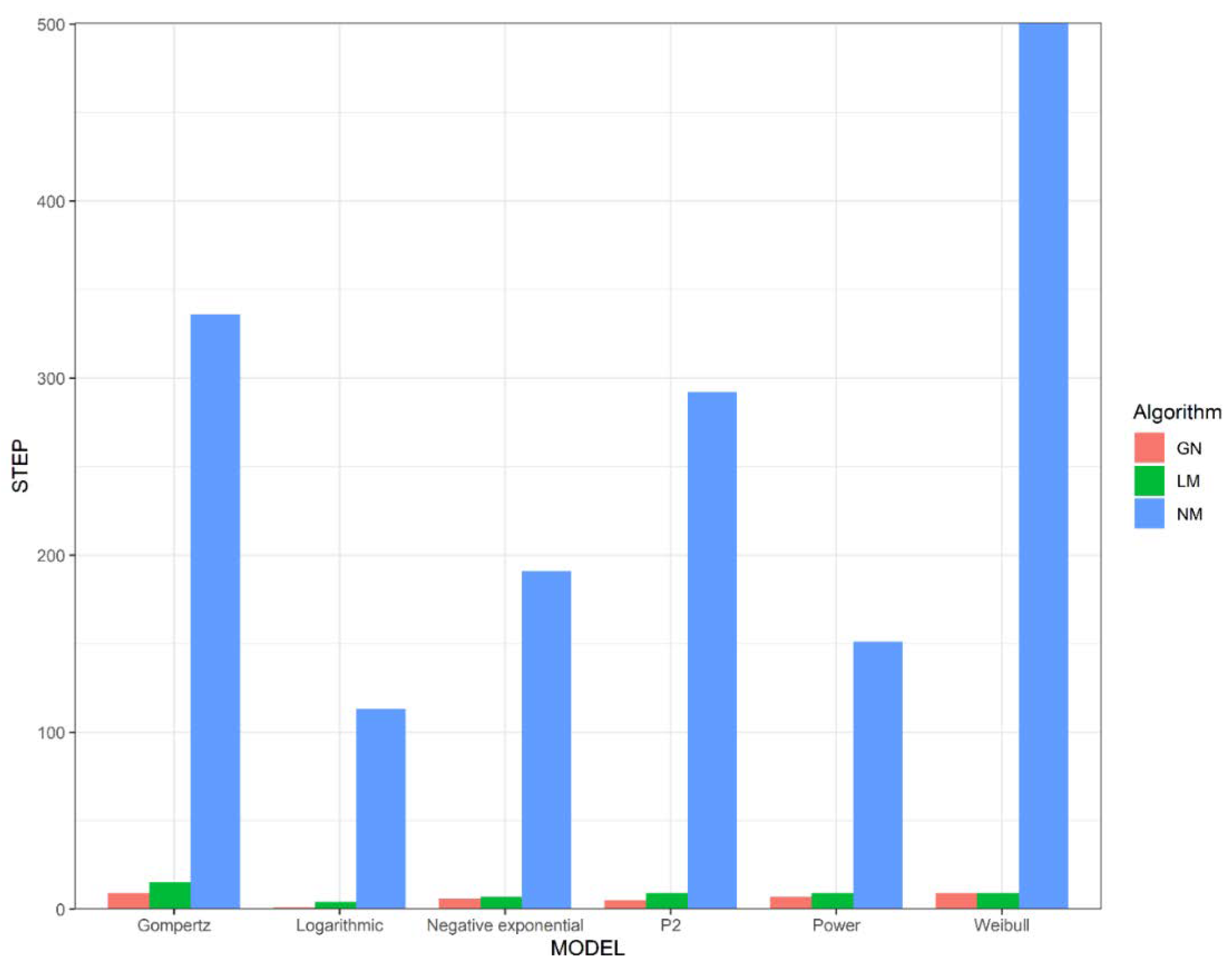
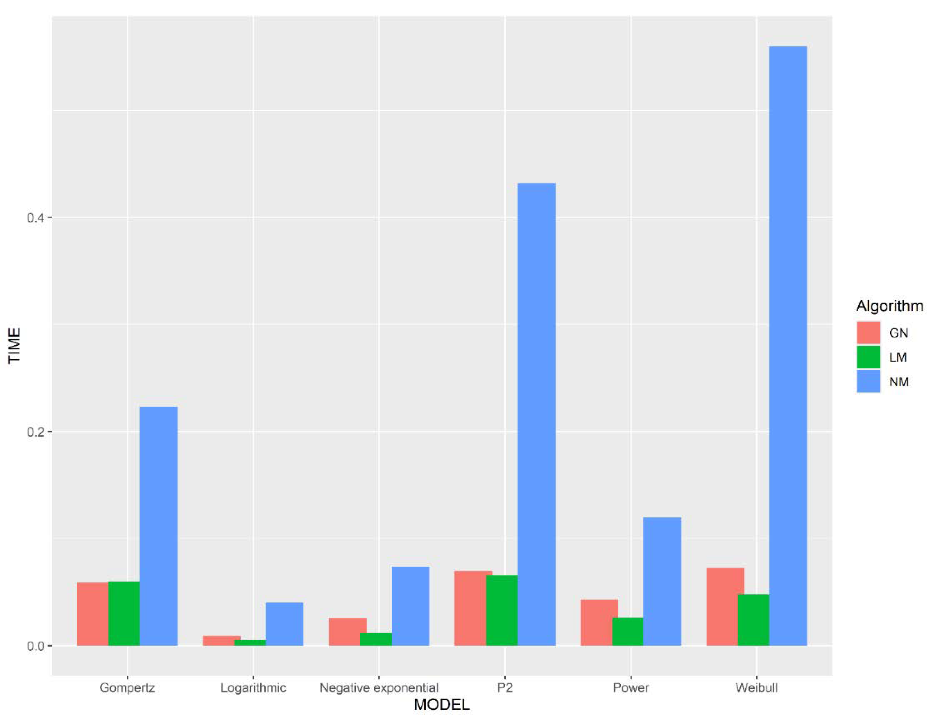
Presently numerous functions have been proposed for modelling SARs, varying in complexity from two to four parameters, in the general form they produce, theoretical background, origin, and justification [23]. We chose six representative models: Power, Gompertz, Negative exponential, Logarithmic models, Weibull, and Persistence function 2. We used the nls function, the optim function, and the nls.Lm function of the minpack.lm package of R software to implement the above algorithms to fit the SAR model. Their applicability is evaluated from three aspects: the number of iterations, the time consumption, and the sensitivity to the initial parameter setting.

In order to investigate the difference in the number of iteration steps and time consumption of different algorithms when fitting the same nonlinear SAR model, we gave the Gauss–Newton method, the Levenberg–Marquardt method, and the Nelder–Mead method the same initial parameters $x_0$ and then processed the same data. To highlight the differences in time consumption and the number of iterations between these algorithms, we simulated species area data for each model by manually setting the model parameters $x_M$ and adding “white noise” items (

Table 1. SAR models used to evaluate the applicability of the different algorithms, and the function with white noise. In this case, the independent variable $\left(A\right)$ is area and the dependent variable $f\left(x\right)$ is the number of species, $b_0$, $b_1$ and $b_2$ are the parameters.

No.	Curve Name	Model	Parameters	Date Simulation	Shape Type
1	Power	$b_0{A}^{b_1}$	2	$b_0{A}^{b_1}+noise$	Convex
2	Gompertz	$b_0\exp \left(-\exp \left(-b_{1}A+b_2\right)\right)$	3	$b_0\exp \left(-\exp \left(-b_{1}A+b_2\right)\right)+noise$	Sigmod
3	Logarithmic	$b_0+b_1\log A$	2	$b_0+b_1\log A+noise$	Convex
4	Negative exponential	$b_0-b_0\exp \left(-b_{1}A\right)$	2	$b_0-b_0\exp \left(-b_{1}A\right)+noise$	Convex
5	Weibull	$b_0\left(1-\exp \left(-b_1{A}^{b_2}\right)\right)$	3	$b_0\left(1-\exp \left(-b_1{A}^{b_2}\right)\right)+noise$	Sigmod
6	Persistence function 2 (P2)	$b_0{A}^{b_1}\exp \left(-b_2/A\right)$	3	$b_0{A}^{b_1}\exp \left(-b_2/A\right)+noise$	Sigmod

). The noise is a random number constructed by R within a certain range. In this way, we generated a dataset in which each data point is distributed around the curve, and we can approximate that $x_M\approx x_T$. We ran forty thousand simulations for each model and then counted the number of iterations and time that were required for different algorithms to iterate from $x_0$ to $x_T$ when processing the simulated data.

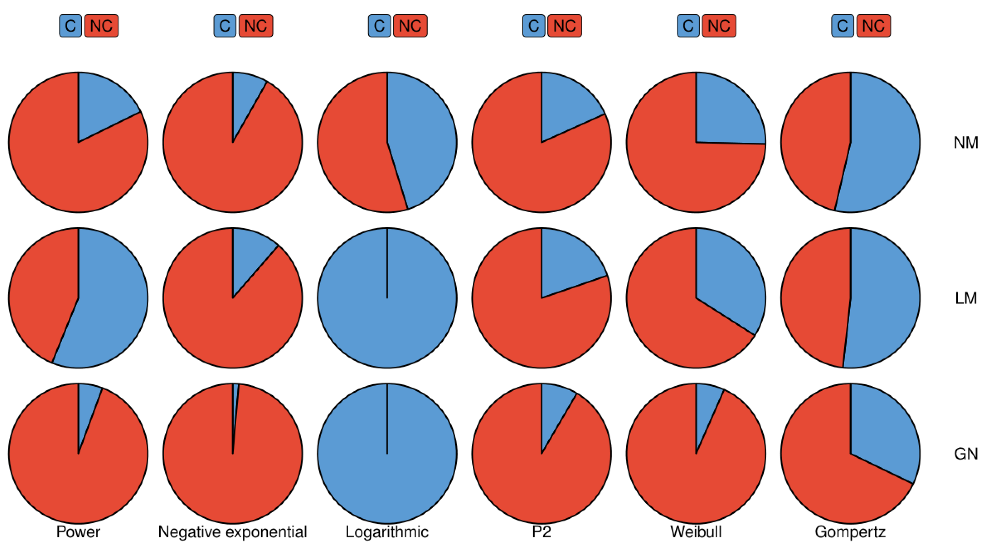
When we study the sensitivity of different algorithms to initial parameter setting, we only need to process general data to show their differences. We used six real species regional data sets from published papers [24,25], including mammal, bird, plant, and insect data. We set a range for each parameter, taking the initial parameters in this range can ensure the algorithm will converge in most cases and will also reflect the difference in sensitivity of different algorithms to the initial parameters. The more times the algorithm converges the less sensitive the algorithm is to initial parameters. We tested all real data sets with all models in Table 1.

3. Results

We studied sensitivity to initial parameters using simulated data (Figure 1 and Figure 2), and the number of iterations and time consumption using real data (Figure 3). As we can see from Figure 1 and Figure 2, the Gauss–Newton and the Levenberg–Marquardt methods require relatively few iteration steps and the Nelder–Mead method requires more iteration steps. Interestingly, even though the Nelder–Mead method needs more iterations to converge, we can see from Figure 1 and Figure 2 that this method consumes less time per iteration than the other algorithms.

The differences in the sensitivity of different algorithms to the initial parameters when fitting the various models to real data are shown in Figure 3: the Levenberg–Marquardt method is least dependent on the initial parameters, followed by the Nelder–Mead method, and the Gauss–Newton method has the strongest dependence. Unexpectedly, when fitting the logarithmic model, the Gauss–Newton method is not sensitive to the initial parameters, and only needs one iteration to converge.

4. Discussion

Many ecologists have applied these algorithms to SAR study [26,27,28]. These algorithms are based on different principles and therefore vary considerably in SAR model fitting. Both the Gauss–Newton’s method and the Levenberg–Marquardt method use the Taylor’s series expansion $L\left(h\right)$ to approximate the nonlinear regression model $F\left(x+h\right)$, and then the regression coefficients $x_0$ are approximated to the optimal coefficient $x_T$ through several iterations to minimize the sum of the squares of $F\left(x\right)$. The Levenberg–Marquardt method adds a damping term and evaluates whether $L\left(h\right)$ is a good approximation of $F\left(x+h\right)$ before each iteration. The Levenberg–Marquardt method can be seen as a combination of the gradient descent method and the Gauss–Newton method [29]. The introduction of the damping factor $\mu$ makes the Levenberg–Marquardt method more flexible. If $\mu$ is close to one, Equation (3) can be approximated as $h_{lm}\approx -\frac{1}{\mu } J\left(x\right)f\left(x\right)$. In such cases, the Levenberg–Marquardt is converted to the gradient descent method. If $\mu$ is close to 0, Equation (3) can be approximately transformed into Equation (3), and the Levenberg–Marquardt method is converted to the Gauss–Newton method. The gradient descent method reduces the sum of the squares of the residuals of $f\left(x\right)$ by updating the parameters in the steepest descent direction. At the beginning of the iteration, the Levenberg–Marquardt method is converted to the gradient descent method and, at the final stage of the iteration process, the Levenberg–Marquardt method is converted to the Gauss–Newton method [29]. Such a strategy can quickly reduce the $F\left(x+h\right)$ in the early stage of the iteration, while still maintaining a fast convergence rate in the final stage. Therefore, even though the Levenberg–Marquardt method requires the evaluation of the similarity of $L\left(h\right)$ and $F\left(x+h\right)$ in each iteration, there is not much difference in the number of iterations and running time between the Levenberg–Marquardt and the Gauss–Newton method.

Unlike the Gauss–Newton method and the Levenberg–Marquardt method, the Nelder–Mead method can take an enormous number of iterations with almost no reduction in $F\left(x\right)$, despite being nowhere near $x_T$, so this method requires more iterative steps to obtain to the $x_T$. Although the Nelder–Mead method requires more iteration steps, this method consumes less time per iteration than the other algorithms. This is because both the Gauss–Newton method and the Levenberg–Marquardt method require the derivation of each parameter of the model to be fitted. Assuming that the model to be fitted has $n$ parameters, both algorithms require $n$ function evaluations per iteration, which undoubtedly requires a lot of time. In contrast, the Nelder–Mead method only requires one or two function evaluations per iteration, which is very important in applications for which each function evaluation is time consuming.

Finally, the sensitivity of these algorithms to the initial parameters is very different, especially between the Gauss–Newton method and the Levenberg–Marquardt method. This difference in sensitivity is driven by the replacement of the Hessian $H$ with $J^{T}J$ in the Gauss–Newton method. Although this change omits a lot of calculations, it also adds instability to the algorithm, because the matrix $J^{T}J$ is only positive semi-definite, which may be singular matrices and ill-conditioned. Poor stability of $h$ will result in non-convergence of the algorithm, but the Levenberg–Marquardt method introduces the damping parameter $\mu >0$, ensuring that the matrix J has full rank. The matrix ($J^{T}J+\mu I)$ is positive define, which means $h_l$ is a descent direction. After each iteration, the Levenberg–Marquardt method evaluates whether the Taylor expansion $L$ approximates the residual function $F$ and prevents the algorithm from converging due to a large $\left|\left|h\right|\right|$. The damping parameter $\mu$ is adjusted according to the quantized result until it reaches the threshold. In contrast, the Nelder–Mead method relies on the initial parameters to generate the initial simplex according to an adjustable strategy, and then converges to the optimal parameters through the deformation of the simplex, so the selection of initial parameters and the strategy of generating simplex will affect the convergence of the algorithm. If the initial simplex is too small, it leads to local search, so the Nelder–Mead method is likely to get stuck. Rigorous analysis of the Nelder–Mead method is a very difficult mathematical problem. A detailed study carried out by Lagarias [20] contains several convergence results in one and two dimensions for strictly convex functions with bounded level sets.

5. Conclusions

After analyzing the number of iterations, time consumption, and sensitivity to the initial parameters, the Levenberg–Marquardt method appears to be the best choice for SAR fitting. It is not the fastest algorithm, but when processing normal data, the difference in time required by different algorithms is negligible. The most important thing is that the Levenberg–Marquardt method has minimal dependence on the initial parameters. In summary, we recommend the Levenberg–Marquardt algorithm for regular SAR model fitting. However, this algorithm requires derivative information similar to the Gauss–Newton method, whereas the Nelder–Mead method iterates by continuously constructing simplexes and does not require any derivative information of the model. Consequently, the Nelder–Mead method is the best choice when the SAR model is a non-smooth function, i.e., when performing a breakpoint species–area regression analysis (as the derivative does not exist, at this point) [30].

References

1. Chave, J.; Muller-Landau, H.C.; Levin, S.A. Comparing Classical Community Models: Theoretical Consequences for Patterns of Diversity. Am. Nat. 2002, 159, 1–23. [Google Scholar] [CrossRef] [PubMed]
2. Ricklefs, R.E.; Bermingham, E. History and the Species-Area Relationship in Lesser Antillean Birds. Am. Nat. 2004, 163, 227–239. [Google Scholar] [CrossRef] [Green Version]
3. Fattorini, S. Beetle Species-Area Relationships and Extinction Rates in Protected Areas. Insects 2020, 11, 646. [Google Scholar] [CrossRef] [PubMed]
4. Willig, M.R.; Kaufman, D.M.; Stevens, R.D. Latitudinal Gradients of Biodiversity: Pattern, Process, Scale, and Synthesis. Annu. Rev. Ecol. Evol. Syst. 2003, 34, 273–309. [Google Scholar] [CrossRef]
5. Preston, F.W. Time and Space and the Variation of Species. Ecology 1960, 41, 611–627. [Google Scholar] [CrossRef]
6. Macarthur, R.H.; Wilson, E.O. An Equilibrium Theory of Insular Zoogeography. Evolution 1963, 17, 373–387. [Google Scholar] [CrossRef]
7. Connor, E.F.; McCoy, E.D. The Statistics and Biology of the Species-Area Relationship. Am. Nat. 1979, 113, 791–833. [Google Scholar] [CrossRef]
8. Arrhenius, O. Species and Area. J. Ecol. 1921, 9, 95–99. [Google Scholar] [CrossRef] [Green Version]
9. Tjørve, E. Shapes and Functions of Species-Area Curves (II): A Review of New Models and Parameterizations. J. Biogeogr. 2009, 36, 1435–1445. [Google Scholar] [CrossRef]
10. Williams, M.R.; Lamont, B.B.; Henstridge, J.D. Species–Area Functions Revisited. J. Biogeogr. 2009, 36, 1994–2004. [Google Scholar] [CrossRef]
11. Matthews, T.J.; Triantis, K.A.; Whittaker, R.J. The Species–Area Relationship: Theory and Application; Cambridge University Press: Cambridge, UK, 2020. [Google Scholar]
12. Fattorini, S. Detecting Biodiversity Hotspots by Species-Area Relationships: A Case Study of Mediterranean Beetles. Conserv. Biol. 2006, 20, 1169–1180. [Google Scholar] [CrossRef] [PubMed]
13. Tjørve, E. Shapes and functions of species–area curves: A review of possible models. J. Biogeogr. 2003, 30, 827–835. [Google Scholar] [CrossRef]
14. Guilhaumon, F.; Mouillot, D.; Gimenez, O. mmSAR: An R-Package for Multimodel Species-Area Relationship Inference. Ecography 2010, 33, 420–424. [Google Scholar] [CrossRef]
15. Matthews, T.J.; Triantis, K.A.; Whittaker, R.J.; Guilhaumon, F. SARS: An R Package for Fitting, Evaluating and Comparing Species–Area Relationship Models. Ecography 2019, 42, 1446–1455. [Google Scholar] [CrossRef] [Green Version]
16. Price, C.J.; Coope, I.D.; Byatt, D. A Convergent Variant of the Nelder–Mead Algorithm. J. Optim. Theory Appl. 2002, 113, 5–19. [Google Scholar] [CrossRef] [Green Version]
17. Levenberg, K. A Method for the Solution of Certain Nonlinear Problems in Least Squares. Q. Appl. Math. 1944, 2, 164–168. [Google Scholar] [CrossRef] [Green Version]
18. Marquardt, D.W. An Algorithm for Least-Squares Estimation of Nonlinear Parameters. J. Soc. Ind. Appl. Math. 1963, 11, 431–441. [Google Scholar] [CrossRef]
19. Ranganathan, A. The Levenberg-Marquardt Algorithm. Tutoral LM Algorithm 2004, 11, 101–110. [Google Scholar]
20. Lagarias, J.C.; Reeds, J.A.; Wright, M.H.; Wright, P.E. Convergence Properties of the Nelder—Mead Simplex Method in Low Dimensions. SIAM J. Optim. 1998, 9, 112–147. [Google Scholar] [CrossRef] [Green Version]
21. Singer, S.; Singer, S. Complexity analysis of Nelder-Mead search iterations. In Proceedings of the 1. Conference on Applied Mathematics and Computation, Dubrovnik, Croatia, 13–18 September 1999; pp. 185–196. [Google Scholar]
22. Singer, S.; Singer, S. Efficient Implementation of the Nelder–Mead Search Algorithm. Appl. Numer. Anal. Comput. Math. 2004, 1, 524–534. [Google Scholar] [CrossRef]
23. Triantis, K.A.; Guilhaumon, F.; Whittaker, R.J. The Island Species-Area Relationship: Biology and Statistics. J. Biogeogr. 2012, 39, 215–231. [Google Scholar] [CrossRef]
24. Newmark, W.D. Species-Area Relationship and Its Determinants for Mammals in Western North American National Parks. Biol. J. Linn. Soc. 2008, 28, 83–98. [Google Scholar] [CrossRef]
25. Chown, S.L.; Gremmen, N.J.M.; Gaston, K.J. Ecological Biogeography of Southern Ocean Islands: Species-Area Relationships, Human Impacts, and Conservation. Am. Nat. 1998, 152, 562–575. [Google Scholar] [CrossRef]
26. Xiang, W.; Lu, S.; Wen, S.; Ding, T.; Wang, B.; Zhou, A.; Huang, F.; Li, X. Sample Effects on Species-Area Relationships of Typical Forests in Karst and Non-karst Mixing Distribution Areas. Guihaia 2015, 35, 309. [Google Scholar]
27. Nikolic, T.; Antonic, O.; Alegro, A.L.; Dobrovic, I.; Bogdanovic, S.; Liber, Z.; Resetnik, I. Plant Species Diversity of Adriatic Islands: An Introductory Survey. Plant Biosyst. 2008, 142, 435–445. [Google Scholar] [CrossRef]
28. Guilhaumon, F.; Gimenez, O.; Gaston, K.J.; Mouillot, D. Taxonomic and Regional Uncertainty in Species-Area Relationships and the Identification of Richness Hotspots. Proc. Natl. Acad. Sci. USA 2008, 105, 15458–15463. [Google Scholar] [CrossRef] [Green Version]
29. Lourakis, M.I.A.; Argyros, A.A. SBA: A Software Package for Generic Sparse Bundle Adjustment. ACM Trans. Math. Softw. 2009, 36, 2. [Google Scholar] [CrossRef]
30. Lomolino, M.V.; Weiser, M. Towards A More General Species-Area Relationship: Diversity on All Islands, Great and Small. J. Biogeogr. 2001, 28, 431–445. [Google Scholar] [CrossRef]
Figure 1. The number of steps required for the algorithms to iterate from the initial parameters x 0 to x T . GN represents the Gauss–Newton method, LM represents the Levenberg–Marquardt method, and NM represents the Nelder–Mead method.
Diversity 14 00212 g001
Figure 2. The time consumption in seconds for the algorithms to iterate from the initial parameters x 0 to x T . GN represents the Gauss–Newton method, LM represents the Levenberg–Marquardt method, and NM represents the Nelder–Mead method.
Diversity 14 00212 g002
Figure 3. The differences in the sensitivity of different algorithms to the initial parameters when fitting the various models. GN represents the Gauss–Newton method, LM represents the Levenberg–Marquardt method, and NM represents the Nelder–Mead method. C indicates that the algorithm converges; NC indicates that the algorithm does not converge.
Diversity 14 00212 g003