
Global Patterns of Earwig Species Richness


Department of Life, Health and Environmental Sciences, University of L’Aquila, Via Vetoio, 67100 L’Aquila, Italy
Diversity 2022, 14(10), 890; https://doi.org/10.3390/d14100890
Submission received: 11 September 2022
/
Revised: 28 September 2022
/
Accepted: 18 October 2022
/
Published: 21 October 2022
Abstract
:One of the most investigated patterns in species diversity is the so-called latitudinal gradient, that is, a decrease in species richness from the equator to the poles. However, few studies investigated this pattern in insects at a global scale because of insufficient taxonomic and biogeographical information. Using estimates of earwig species richness at country level, their latitudinal diversity gradient was modelled globally and for the two hemispheres separately after correcting for differences in country areas. Separate analyses were also conducted for mainland and island countries. All analyses clearly indicated the existence of latitudinal gradients. The most plausible explanation for the observed pattern is the so-called tropical conservatism hypothesis, which postulates (1) a tropical origin of many extant clades, (2) a longer time for cladogenesis in tropical environments thanks to their environmental stability, and (3) a limited ability of historically tropical lineages to adapt to temperate climates. Earwigs probably evolved on Gondwana and secondarily colonized the Northern Hemisphere. This colonization was hampered by both geographical and climatic factors. The Himalayan orogenesis obstructed earwig dispersal into the Palearctic region. Additionally, earwig preferences for warm/hot and humid climates hampered the colonization of temperate regions. Pleistocene glaciation further contributed to reducing diversity at northern latitudes.
1. Introduction
The latitudinal diversity gradient, in which species richness decreases from the equator to the poles, is the most pervasive and notable macroecological pattern on Earth [1,2,3,4,5,6,7,8,9,10,11,12,13]. Although the pattern has been investigated on the most disparate organisms, including, for example, bacteria [14], algae [15], protozoans [16,17,18], molluscs [19,20,21,22], parasite worms [23], polychaetes [24], meiofauna [25], spiders [26] and crustaceans [27,28,29], most research has been focused on plants [30,31,32,33,34,35,36,37,38] and vertebrates [12,31,39,40,41,42,43,44,45,46,47,48,49,50,51,52], whereas comparatively few works have been dedicated to insects, which—with possibly 5.5 million species [53]—are “the most taxonomically intractable of animal classes” [54].
Most of the available research on the latitudinal gradient in insects (including collembolans, currently considered as a separate class of hexapods) deals with patterns observed at a continental [55,56,57,58,59,60,61,62,63,64,65,66,67,68] or even smaller geographical scale [66,69,70,71,72,73,74,75,76,77], whereas only very few studies have been conducted on a global scale [78,79,80,81,82]. Additionally, most studies consider insect families or subfamilies [55,56,59,61,62,63,65,67,68,70,72,74,75,76,80,81], because, for most insect groups, there is insufficient taxonomic and biogeographical information (the so-called Linnean and Wallacean shortfalls, respectively [83]) for large-scale analyses involving higher systematic ranks (see, for example, studies on European collembolans [64], world termites [78], West Palearctic sawflies [84], West Palearctic butterflies [60], North American butterflies [58], Australian butterflies [57], world butterflies [82], and stream-dwelling leaf shredders from various sites around the world [85]).
A notable exception may be represented by earwigs (Dermaptera), an insect order for which there are good estimates of species richness for most of the countries in the world. Dermaptera are a small group of insects including about 2000 known species [86]. Earwigs are mainly hygrophilous and nocturnal insects, finding shelter in crevices of various types, under bark, fallen logs, stones, debris, and dry excrements, as well among mosses, near the base of plants, and in the hallows of trunks [86,87,88]. Most earwigs are omnivorous, feeding on a wide array of living and dead plant and animal matter, as well as spores and parts of fungi [86,87,88]. Some species favour plant material, while others prefer animal food such as small arthropods [86,87]. Few species are anthropophilous, living near or in human settlements [86]. About 40% of earwigs have reduced wings, and even species with well-developed wings rarely fly, which reduces their dispersal ability [86].
Earwigs are known to be mainly associated with warm and humid climates, whereas temperate regions have only a limited number of species [86]. However, no study has attempted to investigate the latitudinal gradient in these insects. The world distribution of earwigs is relatively well known, with reliable estimates of species richness for virtually all the countries in the world [86,89].
The aim of this paper was to use country-level estimates of earwig species richness to test the latitudinal gradient of these insects. In particular, I tested: (1) if the global gradient followed a hump-shaped pattern, with maximum diversity in tropical areas; (2) if diversity decreased poleward in the same way in the two hemispheres; and (3) if mainland and island areas had different patterns.
2. Materials and Methods
Analyses were conducted using values of species richness recorded at the country level (Table S1, Figure S1). These data were taken from Haas [89], who derived his estimates from a detailed scrutiny of literature data, communications, and a personal examination of museum specimens, for a total of about 26,000 records (see Hass [89] for details). This dataset is the best suitable source of information for the global richness of earwigs. Although country borders do not reflect necessarily natural discontinuities, country data are a valuable source of information [82] and are commonly used to detect latitudinal patterns in insects (e.g. [63,64,65,67,76,84]).
Monaco (a city-state with 0 species) was excluded. Country areas were taken from Britannica [90], whereas values of country latitude and longitude (centroids) were extracted from the R package rworldmap [91] (Table S1).
Analyses were developed for the whole data set and for the two hemispheres separately [20]. Because of differences in the size of the countries, country data of species richness could not be directly used to test the latitudinal gradient. Thus, to account for differences in country area, the latitudinal gradient was tested by regressing residuals from species–area relationships against latitude [37,40,42,64,65,92,93].
To model the species–area relationship, I used the linearized (log–log) version of the Arrhenius power function, as this model typically provides the best fit and it is easy to interpret [94,95,96]. The model is:
where S is the species richness recorded in a given country, A is the country area (in km2), and c (the expected number of species per area unit) and z (the slope of the function) are estimated parameters. Because of the presence of zero values, the number of species was log(x + 1)-transformed. Decimal logarithms were used.
log(S) = z log (A) + log(c)
For the whole dataset, a quadratic relationship between diversity and latitude was modelled, as maximum diversity was expected at the centre of the gradient (i.e., around the equator). For the two separate hemispheres, both quadratic and linear functions were tested, with model selection based on values of the corrected Akaike information criterion (AICc). Quadratic models were considered potentially preferable to the linear ones only if ΔAICc < 2. In all cases, ordinary least squares regressions were used. Differences in the slope and in the intercept between the regression lines of the two hemispheres were tested by analysis of covariance; in this case, absolute values of latitude were used (e.g., 10° = 10° N = 10° S). Since species–area relationships may differ between mainland and island systems [97,98,99], analyses were also conducted separately for mainland and island countries. Australia was alternatively considered as mainland or island, but this had virtually no effect on the results.
All calculations were performed with the statistical software R Version 4.0.2 [100]. Regressions were performed using the lm() function. AICc values were calculated using the aictab() function. ANCOVAs were conducted with the aov() function. To take into account multiple testing (the latitudinal diversity pattern was tested nine times), a sequential Bonferroni correction was applied starting with α set at 0.05.
To shed light on potential explanations for the latitudinal gradient, I also explored the role of temperature and precipitation as predictors of area–corrected values of earwig diversity. Both temperature and precipitation may influence species diversity in various ways, because they have close relationships with primary production and biomass, especially in the tropics, and temperature may give rise to species–energy relationships [101,102,103,104,105]. To this end, I used average annual values of temperature and precipitation at the country level (Table S1). As expected, temperature was strongly correlated with latitude (a quadratic function explains about 84% of variance at the global level; Figure S2, Table S2), but was a poor predictor of the area-corrected diversity of earwigs (with less than 1% of explained variance; Figure S3, Table S2). Precipitation was relatively weakly correlated with latitude (a quadratic function explains about 15% of variance at the global level; Figure S2, Table S2), but was a better predictor of the area-corrected diversity of earwigs (with about 25% of explained variance) (Figure S4, Table S2). Given the strong relationship between latitude and temperature, and the poor explanatory power of temperature for earwig diversity, analyses for the two hemispheres and for mainland and island areas separately were conducted only for precipitation.
3. Results
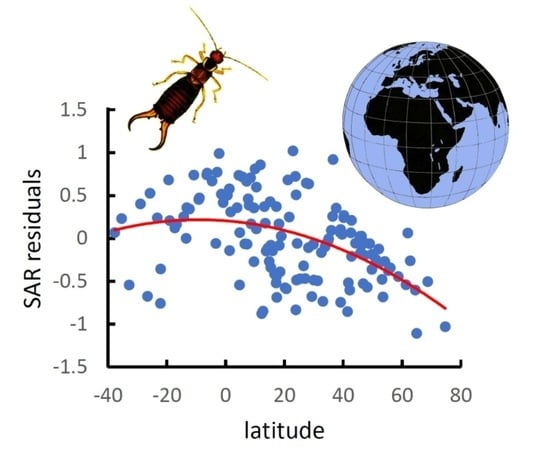
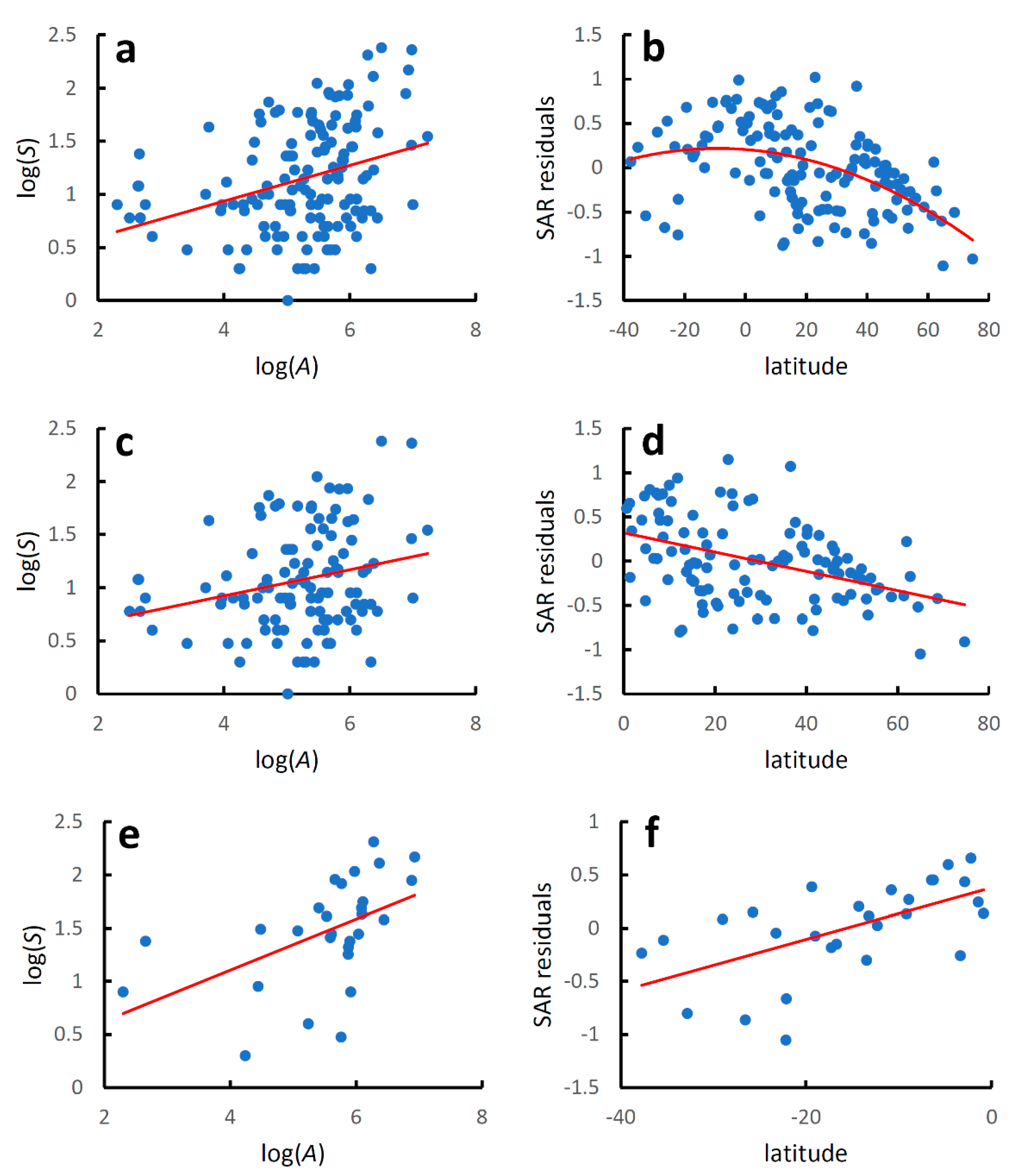
Species richness increased significantly with country area at the global level (Table 1, Figure 1a), although the coefficient of determination was low, which indicates that factors other than area must play an important role in determining the number of species recorded in each country. The latitudinal gradient in species diversity corrected for differences in country areas (residuals from the species–area relationship) followed a hump-shaped pattern, although the coefficient of determination was low (Table 1, Figure 1b).
For the Northern Hemisphere (Table 1, Figure 1c), species richness increased significantly with country area, although the coefficient of determination was even lower than that observed for the whole dataset. Values of species diversity decreased linearly poleward (AICc for a quadratic model: 26.193; AICc for a linear model: 24.092; ΔAICc = 2.101) (Table 1, Figure 1d).
For the Southern Hemisphere (Table 1, Figure 1e), species richness increased significantly with country area, and the coefficient of determination was slightly higher than that observed for the whole dataset. Values of species diversity increased linearly towards the equator (AICc for a quadratic model: 10.226; AICc for a linear model: 7.812; ΔAICc = 2.414) (Table 1, Figure 1f).
Regression lines for the species–area relationship in the two hemispheres did not differ for the slope (F2,137 = 1.510, p = 0.221), but were significantly different for the intercept (F1,138 = 12.600, p = 0.0005). Regression lines for the diversity-latitude relationship in the two hemispheres did not differ neither for the slope (F2,137 = 3.005, p = 0.085) nor for the intercept (F1,138 = 3.187, p = 0.076).
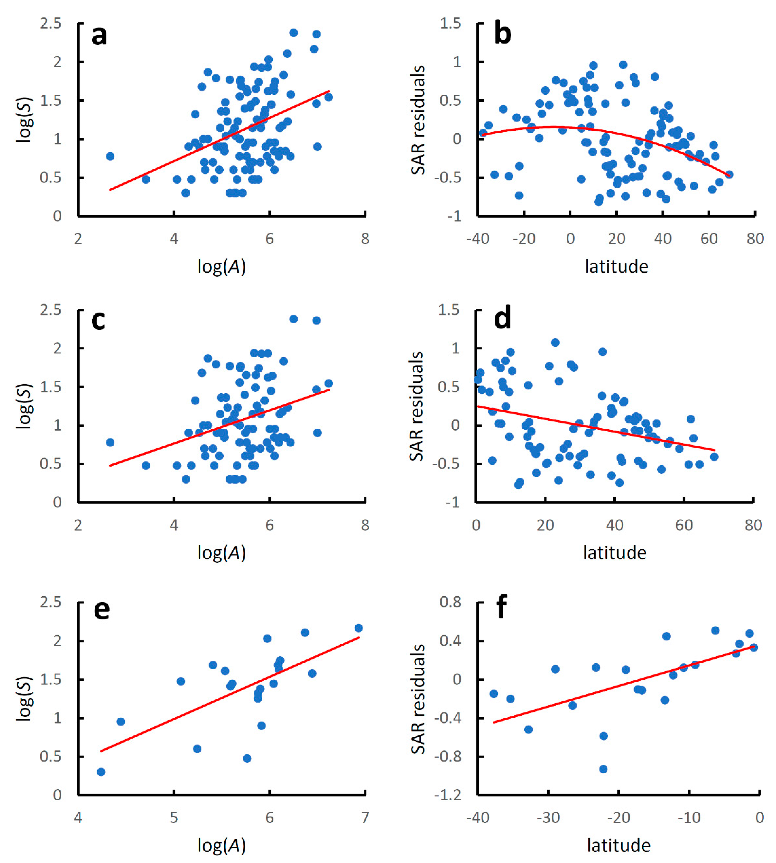
When analysed separately, mainland countries showed a significant increase in species richness with country area at the global level (Table 2, Figure 2a), with a coefficient of determination slightly higher than that found when mainland and island countries were considered together. Regression lines for the species–area relationship in mainland and island countries did not differ for the slope (F2,137 = 1.361, p = 0.085), but were significantly different for the intercepts (F1,138 = 8.871, p = 0.003).
The latitudinal gradient in species diversity followed a hump-shaped pattern, with a coefficient of determination for a quadratic model slightly lower than that obtained for mainland and island countries considered together (Table 2, Figure 2b).
Species richness increased significantly with area in both hemispheres (Table 2, Figure 2c,e), and the coefficients of determinations were higher than those obtained when mainland and island countries were considered together. Regression lines for the species-area relationship in mainland and island countries in the Northern Hemisphere did not differ for the slope (F2,109 = 2.242, p = 0.137) nor for the intercept (F1,110 = 1.587, p = 0.214). Regression lines for the species–area relationship in mainland and island countries in the Southern Hemisphere differed marginally for the slope (F2,24 = 4.184, p = 0.052) and significantly for the intercept (F1,25 = 11.590, p = 0.002).
For both the Northern and Southern Hemispheres, values of species diversity increased linearly towards the equator (Northern Hemisphere: AICc for a quadratic model: 22.732; AICc for a linear model: 20.717; ΔAIC = 2.015; Southern Hemisphere: AICc for a quadratic model: 8.838; AICc for a linear model: 6.298; ΔAICc = 2.539) (Table 2, Figure 2d,f). For the Northern Hemisphere, the coefficient of determination was lower than that observed when mainland and island countries were considered together. In contrast, for the Southern Hemisphere, the fit was superior to that obtained for mainland and island countries taken together. Regression lines for the diversity–latitude relationship in the two hemispheres did not differ neither for the slope (F2,108 = 2.307, p = 0.132) nor for the intercept (F1,109 = 1.430, p = 0.234).
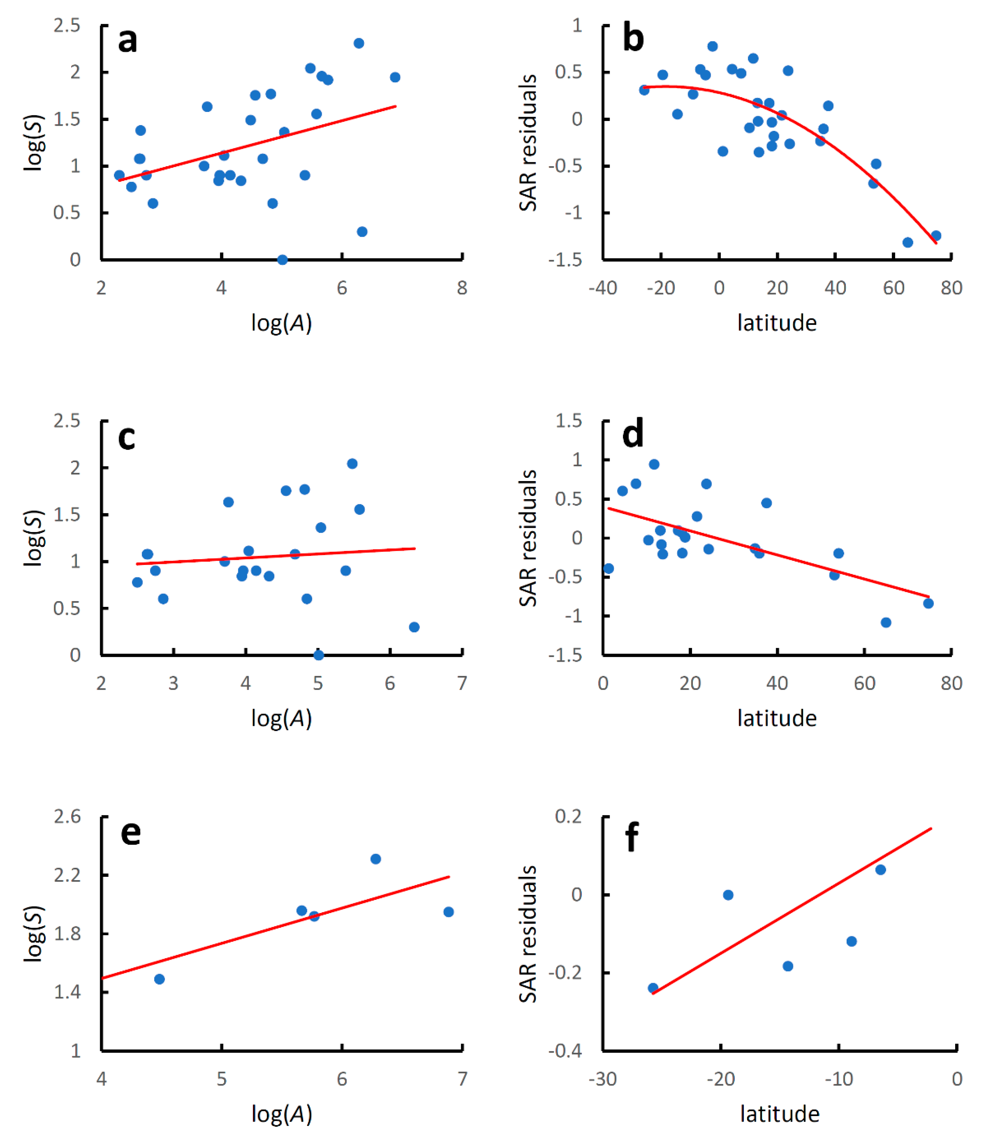
Island countries showed a significant increase in species richness with country area at a global level (Table 3, Figure 3a), with a coefficient of determination slightly higher that that found when mainland and island countries were considered together. The latitudinal gradient of species diversity followed a hump-shaped pattern (Table 3, Figure 3b), with a coefficient of determination substantially higher than that obtained for mainland and island countries considered together.
Species richness increased significantly with area in the Southern Hemisphere, with a relatively high coefficient of determination, whereas the relationship was not significant for the Northern Hemisphere, a possible consequence of the small number of islands included (Table 3, Figure 3c,e).
For the Northern Hemisphere, values of species diversity decreased linearly poleward (AICc for a quadratic model: 8.696; AICc for a linear model: 6.986; ΔAICc = 1.710) (Table 3, Figure 3d). For the Southern Hemisphere diversity increased linearly towards the equator (AICc for a quadratic model: 14.060; AICc for a linear model: 7.084; ΔAICc = 6.977) (Table 3, Figure 3f), but the significance of the relationship did not resist the Bonferroni adjustment. Regression lines for the diversity–latitude relationships in the two hemispheres did not differ, neither for the slope (F2,25 = 0918, p = 0.347) nor for the intercept (F1,26 = 0.086, p = 0.771).
At a global level, temperature was linearly correlated with earwig area–corrected diversity (AICc for a quadratic model: 34.841; AICc for a linear model: 33.503; ΔAICc = 1.338), although the proportion of explained variance was low (r2 for a quadratic model: 0.120; r2 for a linear model: 0.097) (Figure S3, Table S2). Precipitation was a better linear predictor (AICc for a quadratic model: 29.438; AICc for a linear model: 28.813; ΔAICc = 0.625; r2 for a quadratic model: 0.286; r2 for a linear model: 0.241) (Figure S4, Table S2). Precipitation positively influenced values of area-corrected diversity for mainland countries both at a global level and for the two hemispheres taken separately (Figure S4, Table S2). For the island countries, however, positive relationships between precipitation and diversity at a global level and for the Northern Hemisphere did not resist the Bonferroni correction, and no relationship was apparent for the Southern Hemisphere (Figure S4, Table S2).
4. Discussion
Area is typically one of the most important factors explaining variations in species richness, and the species–area relationship is considered one of the most ubiquitous ecological patterns [94,95,96,97,98]. In the present study, at a global level, island and mainland species–area relationships did not differ significantly in their slopes; however, island species richness per unit area (c-values) appeared to be higher than that on the mainlands. This contrasts with expected lower species richness per unit area on islands [5,106,107,108,109,110,111] and suggests that earwigs have either relatively low extinction or high immigration/speciation rates on islands, which counterbalance island isolation. Moreover, as many earwig species are hygrophilous, island faunas may be richer than expected because islands benefit from the presence of a humid (oceanic) climate. In the case of small islands, earwig faunas might have also been largely influenced by recent introduction. However, it is important to note that most of the islands included in this study were in fact very large. Even excluding Australia, the area of the island countries considered in this study varied between 200 km2 and 2,166,086 km2 (median value: 25,724 km2). At this scale, we can expect that isolation promoted within-island radiation. Additionally, most of the islands considered in this study originated through ancient processes of land fragmentation and their fauna might be substantially relictual, and therefore poorly influenced by current immigration/extinction dynamics, as postulated by equilibrium models which assume lower richness on islands [112]. This situation is exacerbated in the Southern Hemisphere, where island species richness per unit area appears to be much higher than that on the mainland; this result, however, should be considered with caution, since the slope is also different (higher in mainland areas), and intercepts can be properly compared only when slopes do not differ. The higher slope of mainland areas may also be unexpected, as the slope of the species–area relationship is usually higher in isolated systems [106,113]. However, this result is in accordance with the highest z-values assumed for interprovincial species–area relationships [113].
When mainland and island countries were considered together, the species–area relationships of the two hemispheres did not differ significantly for the slope, but the Northern Hemisphere had a much higher intercept (i.e., more species per area unit; however, this result should be considered with caution, given the low percentage of variance explained by the model). Both the global species–area relationship, and those for the two hemispheres separately, explained low proportions of variation in species richness (10% of explained variance for the global species–area relationship, 0.6% for the Northern Hemisphere, and 26% for the Southern Hemisphere, respectively). When mainlands and islands were analysed separately, the area explained 17% and 16% of variation in species richness of the mainland and island faunas, respectively.
The species–area relationship in the Southern Hemisphere indicated that area was an important descriptor of species richness here, especially in the island countries (about 83% of explained variance for islands, and 46% for mainlands, respectively). In the Northern Hemisphere, neither the slope nor the intercept differed between mainland and island countries, and in both cases country area was a week predictor of richness (about 1% of explained variance for islands, and 11% for mainlands, respectively). In general, the coefficients of determination of the species–area relationships found in this study show that the explanatory power of area as a predictor of species richness is variable, ranging from less than 1% to more than 83%, with an average of about 24%. This means that the ability of area of predicting richness varies from weak to very strong.
It is not unusual that area alone is a weak or moderate correlate of species richness in macroecological studies. For example, the proportion of variance in species richness explained by area was 0.2–2.5% for liverworts, mosses, and woody plants in Chinese provinces [37]; 41% for collembolans in European mainland countries, 44% in island countries, and 61% for both types merged [64]; 3% for European tenebrionids [67]; 11% for European cerambycids [63]; 23% for butterflies of northern and eastern European countries [114]; and 40% for European clearwing [65].
These results indicate that other factors in addition to area might have more importance in generating large-scale patterns of species diversity. The most obvious geographical variable that may be responsible for global variations in earwig species richness is latitude, as it explains large-scale variation in species richness in the most disparate organisms [1,2,3,4,5,6,7,8,9,10,11,12,13,14,15,16,17,18,19,20,21,22,23,24,25,26,27,28,29,30,31,32,33,34,35,36,37,38,39,40,41,42,43,44,45,46,47,48,49,50,51,52,55,56,57,58,59,60,61,62,63,64,65,66,67,68,69,70,71,72,73,74,75,76,77,78,79,80,81,82].
Values of earwig species richness recorded at country level [86,89] are suggestive of a latitudinal pattern. The analyses presented in this paper clearly support that earwig diversity follows the global latitudinal gradient, peaking in the tropical zone. The amount of variation in area–corrected values of richness explained by latitude ranged from about 11% to 83%. This variability, from relatively low/moderate to high proportions of explained variance, is common in macroecological studies in which latitude is considered as the only correlate of diversity. For example, the proportion of variance in species diversity explained by latitude was 15–18% in marine bacteria [14] and 0.09–30% in diatoms [15] at the global scale; 8% in the non–native species and 30% in the native species of climbing plants of Michigan [36]; 20% in helminth parasites of North America [23]; 4–67% in European collembolans [64]; 56% in New World grasshoppers [56]; 42% in European carabids [62]; 34% in European cerambycids [63]; 30–40% in European clearwing moths [65]; 6% in New World swallowtail butterflies [115]; 1.5–12% in North American butterflies [58]; 3% in Australian butterflies [57]; 48–70% in galling insects [69]; and 16–45% in the New World nonvolant mammals [40] (note that these studies used different statistical approaches, such as ordinary least squares and generalized linear models, and linear or polynomial regressions, with quadratic and even cubic terms). As a measure of geographical position, I have used country centroids. In the case of small countries, centroids provide a rather accurate description of their latitudinal position. However, in the case of countries with a wide latitudinal extent, the use of centroids could produce some bias: most species recorded in a given country are obviously not evenly distributed throughout its entire territory, but might be concentrated in the south. This inaccuracy may contribute to the relatively low values of explained variance.
When the analysis was conducted at the global level and without distinction between mainland and island countries, the highest area-corrected values of earwig diversity were recorded in India and Indonesia. Other countries that ranked high (first 10%) were (in decreasing order of diversity values): the Philippines, Costa Rica, the Democratic Republic of the Congo, Tanzania, Papua New Guinea, Brazil, Brunei, Taiwan, Cameroon, and Panama. Thus, the highest diversity values were concentrated between the tropics, with the exception of China, which appeared as an extra-tropical hotspot of earwig diversity. Separate analyses for the two hemispheres indicated that the latitudinal gradient followed a very similar pattern, with no significant difference in the slopes and intercepts of the regression lines.
When the analysis was restricted to the mainland countries, a hump-shaped pattern was recovered again, with India showing the highest diversity. The other countries included in the first 10% were: Costa Rica, Panama, China, Bhutan, Tanzania, Cameroon, the Democratic Republic of the Congo, Nepal, and Myanmar. Again, diversity appears to be concentrated in inter-tropical latitudes, with the notable exceptions being China, Bhutan, and Nepal. Separate analyses for the two hemispheres indicated that, also in this case, the latitudinal gradient was very similar, with no significant difference in the slopes and intercepts of the regression lines.
A hump-shaped pattern was also found for the island countries, with high values of diversity around the equator. The highest diversity was recorded in Indonesia, followed by the Philippines and Brunei (which constitute the first 10%). Interestingly, with the exception of Japan (which has slightly positive residual and is in the temperate region), all countries with positive residuals are between the tropics.
When analysed separately, both hemispheres showed a clear decrease in diversity from the equator to the poles, but results for the Southern Hemisphere were weaker because of the smaller number of involved countries. However, also in this case, the latitudinal gradients in the two hemispheres were very similar, with no significant difference in the slopes and intercepts of the regression lines.
Overall, these results point to the identification of the following main centres of earwig diversification: (1) tropical South America, with diversity decreasing towards temperate South America and Central and North America; (2) tropical Africa, with decreasing diversity in temperate areas; (3) tropical Asia; and (4) subtropical Asia approximatively below 40° N.
Of course, organisms do not respond to latitude per se, but to different current environmental conditions found at different latitudes, or as a consequence of past events that varied with latitude (such as the incidence of glaciations). Several causal hypotheses have been proposed to explain the latitudinal gradient [1,3,5,6,8,11]. The most general ones include as causal factors:
- (1)
- Time: as tropics were not severely affected by glaciations, they were occupied for longer periods, providing more time for cladogenesis;
- (2)
- Environmental heterogeneity: tropical areas have greater environmental heterogeneity that increases the probability of species coexistence through niche differentiation;
- (3)
- Competition: while temperate populations may be more controlled by abiotic factors (seasonality), tropical populations are more regulated by biotic interactions, such as competition, which increases species diversity through specialization;
- (4)
- Predation: tropics have more predators that maintain prey species at low densities, thus decreasing competition among prey species and hence increasing the coexistence of prey species (this hypothesis suggests a mechanism exactly opposite to that of the competition hypothesis);
- (5)
- Productivity: tropics support more species because more resources are available, allowing for more specialization;
- (6)
- Environmental (climatic) stability: severe and/or unpredictable climates tend to have lower habitat diversity, whereas stable climates tend to present higher habitat diversity, which, in turn, promotes species diversity (as in the environmental heterogeneity hypothesis).
These explanations are not necessarily alternative, but some may act in concert and can be integrated with other plausible mechanisms to formulate even more compressive hypotheses. For example, according to the tropical conservatism hypothesis [116], current high tropical diversity might result from: (i) tropical origin of many lineages, as tropical regions had a greater geographical extent until relatively recently (less than 40 million years ago, when temperate zones increased in size), (ii) longer time for cladogenesis in tropical environments, thanks to their environmental stability, and (iii) the limited ability of organisms from historically tropical lineages to adapt to temperate climates and then to dispersal poleward.
On the basis of earwig biology [86], competition, predation and productivity can be hardly considered major drivers for the latitudinal diversity pattern in these insects. Most earwigs are omnivores or at least generalists (a few species are epizoic commensals), which can occupy very different biotopes, so it is difficult to speculate that competition for food or space may be a major driver promoting speciation. For the same reasons, productivity can be hardly evoked as an important factor for the latitudinal gradient. At the global level, earwig diversity was very weakly correlated with temperature, which suggests that available energy is not a major factor for the latitudinal patterns of diversity of earwigs, despite their preference for warm climates. Consistent with their preference for humid climates, earwig diversity was positively influenced by precipitation. However, precipitation was uncorrelated with latitude, and thus the relationship between diversity and precipitation cannot be evoked as a major explanation for the latitudinal pattern. Earwigs are preyed on by many animals (such as centipedes, beetles, assassin bugs, spiders, toads, lizards, snakes, birds, insectivorous mammals and bats) which, however, do not specialize on them; therefore, it is difficult to speculate that predation may be a strong explanation for earwig diversification in the tropics. Because of their generalism in biotope occupancy, it is difficult to associate the higher diversity of earwigs in the tropics with environmental heterogeneity. Thus, historical reasons seem to offer the most decent explanations to the observed patterns. In particular, the historical biogeography of earwigs, and their ecological preferences for warm/hot and humid climates, support the tropical conservatism hypothesis as the most reasonable explanation for the observed latitudinal patterns.
According to Popham and Manly [117] and Popham [118] earwigs evolved on Gondwana (the supercontinent that grouped most of the land masses in today’s southern hemisphere, including Antarctica, South America, Africa and Madagascar), and secondarily colonized the northern hemisphere. The earwig distribution after Gondwana fragmentation occurred in the Jurassic has been largely affected by climatic conditions, which have largely hampered the colonization of the Northern Hemisphere which was (and is) not very suitable to insects such as earwigs, since these insects are associated with warm/hot and humid climates, with low capability to adapt to temperate/cold climates. The Himalayan orogenesis also created a barrier that largely prevented earwig dispersion into the Palearctic region, which may explain the low diversity values recorded in most countries in this biogeographical realm. The Palearctic region, however, shows two main centres of differentiation: one corresponding to Eastern Asia between the Tropic of Cancer and 40° N, and the other in the Mediterranean Basin, with the Iberian, Italian and Balkan peninsulas showing relatively high diversity. These two areas correspond to the two centres of earwig diversity already recognized almost a century ago by Bey–Bienko [119]: one in an eastern Asian region including the Ussuri basin, Northern China, Japan, Korea, Manchuria and Tibet (and thus corresponding to the “paleoarchearctic” region of Semenov Tian–Shanskij [120]), and the other in the Mediterranean Basin. Actually, the presence of a diversity centre in Eastern Asia, south of the Himalayas, supports the idea that earwig dispersion was blocked northwards by the Himalayan orogenesis, but permitted through the deep river valleys of Southeast Asia, allowing earwigs to invade (and differentiate in) Tibet, China and Japan [118]). The high diversity of earwigs in the Mediterranean, and specifically in South European countries, can be explained by their role as refugial centres during Pleistocene glaciations [121,122,123,124,125,126]. In the future, it would be interesting to test this inferred scenario through phylogeographic analyses based on molecular data, which are, however, still rare for earwigs [127].
5. Conclusions
A global analysis of earwig species richness recorded at the country level clearly indicates the existence of a latitudinal gradient, in which diversity decreases, in both hemispheres, from the equator to the poles. The most plausible explanation for this pattern is the so-called tropical conservatism hypothesis, which postulates a current high tropical diversity as a result of (i) tropical origins of many extant clades, (ii) a longer time for cladogenesis in tropical environments thanks to their environmental stability, and (iii) the limited ability of organisms from historically tropical lineages to adapt to temperate climate. The expansion of temperate/cold habitats in the past 40 million years, as well as mountain uplifts and, more recently, the retreat of high-latitude glaciations, have all contributed to the latitudinal distribution of earwig diversity. Historical reconstructions of earwig biogeography suggest that earwigs evolved on Gondwana and secondarily colonized the Northern Hemisphere. However, this colonization was hampered by both geographical and climatic factors. The Himalayan orogenesis obstructed earwig dispersal into the Palearctic region. Additionally, earwig preferences for warm and humid climates hampered these insects from adapting to temperate and cold climates, which largely prevented the colonization of temperate regions. Pleistocene glaciations further contributed to reducing earwig diversity at northern latitudes.
An important limit of the research presented in this paper is that it is entirely based on current distributional patterns, which may have been affected by rapid long-distance dispersal events, and hence do not necessarily reflect historical factors. There are some earwig species that have great dispersal capabilities and have become widely distributed. For example, Labidura riparia (Pallas, 1773), which is mainly associated with costal sandy shores, is prone to be dispersed with drifting materials. A few species have attained wide distributions thanks to human transportation. For example, Forficula auricularia Linnaeus, 1758, which lives near or in human settlements, was imported into North America between the 19th and 20th century [128]. Labia minor (Linnaeus, 1758), which lives in dung heaps from horses and cows, possibly extended its distribution from Asia around the globe via horses and cows [86]. Chelisoches morio (Fabricius, 1775) and Euborellia annulipes (Lucas, 1847) are other species that attained cosmopolitan distributions. However, these widely distributed species are a minority of cases. Earwigs are not synanthropic, and possibly because of a lack of flight activity, most species have a weak tendency to extend their ranges. This is shown, for example, by the high incidence of regional endemism [86,127]. High endemicity in these insects suggests that their distributions convey robust historical signals, although long-distance dispersal may act as an important confounding factor, and great care must be placed in inferring historical scenarios from current distributions alone.
Because the areas (countries) considered in this study had different sizes, residuals from species–area relationships fitted with the power function were used as area-corrected values of richness to investigate latitudinal patterns. The use of different functions to fit the species–area relationship would obviously produce different sets of residuals. Thus, results will change according to the function(s) used to fit the species–area relationship. In this paper, the linearized version of the power function was used to fit the species–area relationship in all cases as this model typically provides the best fit and it is easy to interpret [94,95,96]. However, it would be useful in the future to explore the effect of using other competitive models.
In this study, I did not consider topographical factors (such as elevation and distance to the coast), climatic factors, or other environmental variables (vegetation setting) which may have important confounding effects on the latitudinal gradients. For instance, since earwigs are mainly hygrophilous insects, countries with a dry continental climate may have less earwig species than those with a humid climate situated at the same latitudes. This may explain, for example, the very small number of species found in Mongolia (a country dominated by extreme continental climatic conditions), despite the large size of this country.
The historical scenarios inferred in this paper from the observed patterns and earwig biology might serve as working hypothesis for future research incorporating phylogenetic information from molecular data, fine-grained distributional data, and environmental variables.
Supplementary Materials
The following supporting information can be downloaded at: https://www.mdpi.com/article/10.3390/d14100890/s1: Table S1: Longitude, latitude, area, average temperature, average precipitation and number of earwig species for countries classified as mainlands or islands. Table S2: Latitudinal patterns of variation of average annual temperature and precipitation (second-order polynomial regressions), and relationships between earwig diversity (residuals from the species–area relationships; Tables 1–3) and precipitation (linear regressions). Figure S1: Global pattern of earwig species richness by country. Figure S2: Latitudinal patterns of variation in average annual temperature (a) and precipitation (b) by country. Regression equations are given in Table S2. Figure S3: Relationship between earwig diversity and average annual temperature at global level. Regression equation is given in Table S2. Figure S4: Relationships between earwig diversity and precipitation. Regression equations are given in Table S2.
Funding
This research received no external funding.
Institutional Review Board Statement
Not applicable.
Informed Consent Statement
Not applicable.
Data Availability Statement
The data presented in this study are available in Table S1.
Acknowledgments
I am grateful to three anonymous reviewers for their comments on a previous version of this paper.
Conflicts of Interest
The author declares no conflict of interest.
References
- Pianka, E.R. Latitudinal Gradients in Species Diversity: A Review of Concepts. Am. Nat. 1966, 100, 33–46. [Google Scholar] [CrossRef]
- Rohde, K. Latitudinal gradients in species diversity: The search for the primary cause. Oikos 1992, 65, 514–527. [Google Scholar] [CrossRef] [Green Version]
- Willig, M.R.; Kaufman, D.M.; Stevens, R.D. Latitudinal gradients of biodiversity: Pattern, process, scale, and synthesis. Annu. Rev. Ecol. Evol. Syst. 2003, 34, 273–309. [Google Scholar] [CrossRef]
- Hillebrand, H. On the generality of the latitudinal diversity gradient. Am. Nat. 2004, 163, 192–211. [Google Scholar] [CrossRef] [PubMed] [Green Version]
- Lomolino, M.V.; Riddle, B.R.; Whittaker, R.J.; Brown, J.H. Biogeography, 4th ed.; Sinauer Associates Inc.: Sunderland, MA, USA, 2010. [Google Scholar]
- Brown, J.H. Why are there so many species in the tropics? J. Biogeogr. 2014, 41, 8–22. [Google Scholar] [CrossRef] [PubMed] [Green Version]
- Gillman, L.N.; Wright, S.D. Species richness and evolutionary speed: The influence of temperature, water and area. J. Biogeogr. 2014, 41, 39–51. [Google Scholar] [CrossRef]
- Fine, P.V.A. Ecological and evolutionary drivers of geographic variation in species diversity. Annu. Rev. Ecol. Evol. Syst. 2015, 46, 369–392. [Google Scholar] [CrossRef] [Green Version]
- Jablonski, D.; Huang, S.; Roy, K.; Valentine, J.W. Shaping the latitudinal diversity gradient: New perspectives from a synthesis of paleobiology and biogeography. Am. Nat. 2017, 189, 1–12. [Google Scholar] [CrossRef] [Green Version]
- Schemske, D.W.; Mittelbach, G.G. “Latitudinal gradients in species diversity”: Reflections on Pianka’s 1966 article and a look forward. Am. Nat. 2017, 189, 599–603. [Google Scholar] [CrossRef] [PubMed]
- Kinlock, N.L.; Prowant, L.; Herstoff, E.M.; Foley, C.M.; Akin-Fajiye, M.; Bender, N.; Umarani, M.; Ryu, H.Y.; Sen, H.Y.; Gurevitch, J.; et al. Explaining global variation in the latitudinal diversity gradient: Meta-analysis confirms known patterns and uncovers new ones. Glob. Ecol. Biogeogr. 2018, 27, 125–141. [Google Scholar] [CrossRef]
- Saupe, E.E.; Myers, C.E.; Townsend Peterson, A.; Soberon, J.; Singarayer, J.; Valdes, P.; Qiao, H. Spatio–temporal climate change contributes to latitudinal diversity gradients. Nat. Ecol. Evol. 2019, 3, 1419–1429. [Google Scholar] [CrossRef] [PubMed] [Green Version]
- Beaugrand, G.; Kirby, R.; Goberville, E. The mathematical influence on global patterns of biodiversity. Ecol. Evol. 2020, 10, 6494–6511. [Google Scholar] [CrossRef] [PubMed]
- Fuhrman, J.A.; Steele, J.A.; Hewson, I.; Schwalbach, M.S.; Brown, M.V.; Green, J.L.; Brown, J.H. A latitudinal diversity gradient in planktonic marine bacteria. Proc. Natl. Acad. Sci. USA 2008, 105, 7774–7778. [Google Scholar] [CrossRef] [PubMed] [Green Version]
- Hillebrand, H.; Azovsky, A.I. Body size determines the strength of the latitudinal diversity gradient. Ecography 2001, 24, 251–256. [Google Scholar] [CrossRef]
- Culver, S.J.; Buzas, M.A. Global latitudinal species diversity gradient in deep–sea benthic foraminifera. Deep-Sea Res. 2000, 47, 259–275. [Google Scholar] [CrossRef]
- Dolan, J.R.; Gallegos, C.L. Estuarine diversity of tintinnids (planktonic ciliates). J. Plankton Res. 2001, 23, 1009–1027. [Google Scholar] [CrossRef] [Green Version]
- Nunn, C.L.; Altizer, S.M.; Sechrest, W.; Cunningham, A.A. Latitudinal Gradients of Parasite Species Richness in Primates. Divers. Distrib. 2005, 11, 249–256. [Google Scholar] [CrossRef]
- Flessa, K.W.; Jablonski, D. Biogeography of Recent marine bivalve molluscs and its implications for paleobiogeography and the geography of extinction: A progress report. Histor. Biol. 1995, 10, 25–47. [Google Scholar] [CrossRef]
- Fortes, R.R.; Absalão, R.S. The Applicability of Rapoport’s Rule to the Marine Molluscs of the Americas. J. Biogeogr. 2004, 31, 1909–1916. [Google Scholar] [CrossRef]
- Jablonski, D.; Roy, K.; Valentine, J.W. Out of the tropics: Evolutionary dynamics of the latitudinal diversity gradient. Science 2006, 314, 102–106. [Google Scholar] [CrossRef] [PubMed]
- Jablonski, D.; Belanger, C.L.; Berke, S.K.; Huang, S.; Krug, A.Z.; Roy, K.; Tomašových, A.; Valentine, J.W. Out of the tropics, but how? Fossils, bridge species, and thermal ranges in the dynamics of the marine latitudinal diversity gradient. Proc. Natl. Acad. Sci. USA 2013, 110, 10487–10494. [Google Scholar] [CrossRef] [Green Version]
- Johnson, P.T.J.; Haas, S.E. Why do parasites exhibit reverse latitudinal diversity gradients? Testing the roles of host diversity, habitat and climate. Glob. Ecol. Biogeogr. 2021, 30, 1810–1821. [Google Scholar] [CrossRef]
- Moreno, R.A.; Labra, F.A.; Cotoras, D.D.; Camus, P.A.; Gutiérrez, D.; Aguirre, L.; Rozbaczylo, N.; Poulin, E.; Lagos, N.A.; Zamorano, D.; et al. Evolutionary drivers of the hump–shaped latitudinal gradient of benthic polychaete species richness along the Southeastern Pacific coast. PeerJ 2021, 9, e12010. [Google Scholar] [CrossRef]
- Kotwicki, L.; Szymelfenig, M.; De Troch, M.; Urban–Malinga, B.; Węsławski, J.M. Latitudinal biodiversity patterns of meiofauna from sandy littoral beaches. Biodivers. Conserv. 2005, 14, 461–474. [Google Scholar] [CrossRef]
- Piel, W.H. The global latitudinal diversity gradient pattern in spiders. J. Biogeogr. 2018, 45, 1896–1904. [Google Scholar] [CrossRef]
- Reid, J.W. Latitudinal diversity patterns of continental benthic copepod species assemblages in the Americas. Hydrobiologia 1994, 292/293, 341–349. [Google Scholar] [CrossRef]
- Dworschak, P.C. Global diversity in the Thalassinidea (Decapoda). J. Crustac. Biol. 2000, 20, 238–245. [Google Scholar] [CrossRef] [Green Version]
- Chiu, W.T.R.; Yasuhara, M.; Cronin, T.M.; Hunt, G.; Gemery, L.; Wei, C.L. Marine latitudinal diversity gradients, niche conservatism and out of the tropics and Arctic: Climatic sensitivity of small organisms. J. Biogeogr. 2020, 47, 817–828. [Google Scholar] [CrossRef]
- Enquist, B.J.; Niklas, K.J. Invariant scaling relations across tree–dominated communities. Nature 2001, 410, 655–660. [Google Scholar] [CrossRef]
- Sax, D.F. Latitudinal gradients and geographic ranges of exotic species: Implications for biogeography. J. Biogeogr. 2001, 28, 139–150. [Google Scholar] [CrossRef]
- Qian, H.; Song, J.S.; Krestov, P.; Guo, Q.; Wu, Z.; Shen, X.; Guo, X. Large–scale phytogeographical patterns in East Asia in relation to latitudinal and climatic gradients. J. Biogeogr. 2003, 30, 129–141. [Google Scholar] [CrossRef] [Green Version]
- Davies, T.J.; Barraclough, T.G.; Savolainen, V.; Chase, M.W. Environmental causes for plant biodiversity gradients. Philos. Trans. R. Soc. Lond. B Biol. Sci. 2004, 359, 1645–1656. [Google Scholar] [CrossRef]
- Mutle, J.; Barthlott, W. Patterns of vascular plant diversity at continental to global scales. Biol. Skr. 2005, 55, 521–531. [Google Scholar]
- Kerkhoff, A.J.; Moriarty, P.E.; Weiser, M.D. The latitudinal species richness gradient in New World woody angiosperms is consistent with the tropical conservatism hypothesis. Proc. Natl Acad. Sci. USA 2014, 111, 8125–8130. [Google Scholar] [CrossRef] [PubMed] [Green Version]
- Burnham, R.J.; Santanna, C.V. Distribution, diversity, and traits of native, exotic, and invasive climbing plants in Michigan. Brittonia 2015, 67, 350–370. [Google Scholar] [CrossRef]
- Chen, S.B.; Ferry Slik, J.W.; Gao, J.; Mao, L.F.; Bi, M.J.; Shen, M.W.; Zhou, K.X. Latitudinal diversity gradients in bryophytes and woody plants: Roles of temperature and water availability. J Syst. Evol. 2015, 53, 535–545. [Google Scholar] [CrossRef]
- Liu, H.; Yu, R.; Huang, J.; Liu, Y.; Zang, R.; Guo, Z.; Ding, Y.; Lu, X.; Li, Q.; Chen, H.Y.H. Latitudinal diversity gradients and Rapoport effects in Chinese endemic woody seed plants. Forests 2020, 11, 1029. [Google Scholar] [CrossRef]
- Oberdorff, T.; Guégan, J.-F.; Hugueny, B. Global scale patterns of fish species richness in rivers. Ecography 1995, 18, 345–352. [Google Scholar] [CrossRef]
- Kaufman, D.M.; Willig, M.R. Latitudinal patterns of mammalian species richness in the New World: The effects of sampling method and faunal group. J. Biogeogr. 1998, 25, 795–805. [Google Scholar] [CrossRef]
- Hawkins, B.A.; Porter, E.E.; Diniz–Filho, J.A.F. Productivity and history as predictors of the latitudinal diversity gradient of terrestrial birds. Ecology 2003, 84, 1608–1623. [Google Scholar] [CrossRef] [Green Version]
- Patten, M.A. Correlates of species richness in North American bat families. J. Biogeogr. 2004, 31, 975–985. [Google Scholar] [CrossRef]
- Stevens, R.D. Untangling latitudinal richness gradients at higher taxonomic levels: Familial perspectives on the diversity of New World bat communities. J. Biogeogr. 2004, 31, 665–674. [Google Scholar] [CrossRef]
- Turner, J.R.G.; Hawkins, B.A. The global biodiversity gradient. In Frontiers of Biogeography: New Directions in the Geography of Nature; Lomolino, M.V., Heaney, L.R., Eds.; Sinauer Associates Inc.: Sunderland, MA, USA, 2004; pp. 171–190. [Google Scholar]
- Buckley, L.B.; Jetz, W. Environmental and historical constraints on global patterns of amphibian richness. Proc. R. Soc. Lond. Ser. B 2007, 274, 1167–1173. [Google Scholar] [CrossRef] [PubMed]
- Hawkins, B.A.; Diniz–Filho, J.A.; Jaramillo, C.A.; Soeller, S.A. Climate, niche conservatism, and the global bird diversity gradient. Am. Nat. 2007, 170, S16–S27. [Google Scholar] [CrossRef] [PubMed]
- Fisher, J.A.; Frank, K.T.; Petrie, B.; Leggett, W.C.; Shackell, N.L. Temporal dynamics within a contemporary latitudinal diversity gradient. Ecol. Lett. 2008, 11, 883–897. [Google Scholar] [CrossRef] [PubMed]
- Schipper, J.; Chanson, J.S.; Chiozza, F.; Cox, N.A.; Hoffmann, M.; Katariya, V.; Lamoreux, J.; Rodrigues, A.S.; Stuart, S.N.; Temple, H.J.; et al. The status of the world’s land and marine mammals: Diversity, threat, and knowledge. Science 2008, 322, 225–230. [Google Scholar] [CrossRef] [PubMed] [Green Version]
- Rolland, J.; Condamine, F.L.; Jiguet, F.; Morlon, H. Faster speciation and reduced extinction in the tropics contribute to the mammalian latitudinal diversity gradient. PLoS Biol. 2014, 12, e1001775. [Google Scholar] [CrossRef]
- Rolland, J.; Condamine, F.L.; Beeravolu, C.R.; Jiguet, F.; Morlon, H. Dispersal is a major driver of the latitudinal diversity gradient of Carnivora. Glob. Ecol. Biogeogr. 2015, 24, 1059–1071. [Google Scholar] [CrossRef]
- Pulido–Santacruz, P.; Weir, J.T. Extinction as a driver of avian latitudinal diversity gradients. Evolution 2016, 70, 860–872. [Google Scholar] [CrossRef]
- Hanly, P.J.; Mittelbach, G.G.; Schemske, D.W. Speciation and the latitudinal diversity gradient: Insights from the global distribution of endemic fish. Am. Nat. 2017, 189, 604–615. [Google Scholar] [CrossRef] [Green Version]
- Stork, N.E. How many species of insects and other terrestrial arthropods are there on Earth? Annu. Rev. Entomol. 2018, 63, 31–45. [Google Scholar] [CrossRef] [PubMed]
- Eggleton, P. The state of the world’s insects. Ann. Rev. Environ. Resour. 2020, 45, 61–82. [Google Scholar] [CrossRef]
- Janzen, D.H. The peak in North American ichneumonid species richness lies between 38° and 42° N. Ecology 1981, 62, 532–537. [Google Scholar] [CrossRef]
- Davidowitz, G.; Rosenzweig, M.L. The latitudinal gradient of species diversity among North American grasshoppers (Acrididae) within a single habitat: A test of the spatial heterogeneity hypothesis. J. Biogeogr. 1998, 25, 553–560. [Google Scholar] [CrossRef]
- Dingle, H.; Rochester, W.; Zalucki, M. Relationships among climate, latitude and migration: Australian butterflies are not temperate–zone birds. Oecologia 2000, 124, 196–207. [Google Scholar] [CrossRef]
- Kocher, S.D.; Williams, E.H. The diversity and abundance of north American butterflies vary with habitat disturbance and geography. J. Biogeogr. 2000, 27, 785–794. [Google Scholar] [CrossRef]
- Lobo, J.M. Species diversity and composition of dung beetle (Coleoptera: Scarabaeoidea) assemblages in North America. Canadian Entomologist 2000, 132, 307–321. [Google Scholar] [CrossRef]
- Hawkins, B.A.; Porter, E.E. Water–energy balance and the geographic pattern of species richness of western Palearctic butterflies. Ecol. Entomol. 2003, 28, 678–686. [Google Scholar] [CrossRef] [Green Version]
- Rodriguero, M.S.; Gorla, D.E. Latitudinal Gradient in Species Richness of the New World Triatominae (Reduviidae). Glob. Ecol. Biogeogr. 2004, 13, 75–84. [Google Scholar] [CrossRef]
- Schuldt, A.; Assmann, T. Environmental and historical effects on richness and endemism patterns of carabid beetles in the western Palaearctic. Ecography 2009, 32, 705–714. [Google Scholar] [CrossRef]
- Baselga, A. Determinants of species richness, endemism and turnover in European longhorn beetles. Ecography 2008, 31, 263–271. [Google Scholar] [CrossRef]
- Ulrich, W.; Fiera, C. Environmental correlates of species richness of European springtails (Hexapoda: Collembola). Acta Oecol. 2009, 35, 45–52. [Google Scholar] [CrossRef]
- Bąkowski, M.; Ulrich, W.; Laštůvka, Z. Environmental correlates of species richness of Sesiidae (Lepidoptera) in Europe. Eur. J. Entomol. 2010, 107, 563–570. [Google Scholar] [CrossRef] [Green Version]
- Hawkins, B.A. Multiregional comparison of the ecological and phylogenetic structure of butterfly species richness gradients. J. Biogeogr. 2010, 37, 647–656. [Google Scholar] [CrossRef]
- Fattorini, S.; Ulrich, W. Drivers of species richness in European Tenebrionidae (Coleoptera). Acta Oecol. 2012, 36, 255–258. [Google Scholar] [CrossRef]
- Burington, Z.L.; Inclán–Luna, D.J.; Pollet, M.; Stireman, J.O., III. Latitudinal patterns in tachinid parasitoid diversity (Diptera: Tachinidae): A review of the evidence. Insect Conserv. Divers. 2020, 13, 419–431. [Google Scholar] [CrossRef] [Green Version]
- Fernandes, G.W.; Price, P.W. Biogeographical gradients in galling species richness. Tests of hypotheses. Oecologia 1988, 76, 161–167. [Google Scholar] [CrossRef]
- Cushman, J.; Lawton, J.; Manly, B. Latitudinal patterns in European ant assemblages: Variation in species richness and body size. Oecologia 1993, 95, 30–37. [Google Scholar] [CrossRef]
- Andrew, N.R.; Hughes, L. Diversity and assemblage structure of phytophagous Hemiptera along a latitudinal gradient: Predicting the potential impacts of climate change. Glob. Ecol. Biogeogr. 2005, 14, 249–262. [Google Scholar] [CrossRef]
- Fattorini, S. Testing the latitudinal gradient: A narrow scale analysis of tenebrionid richness (Coleoptera, Tenebrionidae) in the Aegean archipelago (Greece). Ital. J. Zool. 2006, 73, 203–211. [Google Scholar] [CrossRef]
- Cancello, E.M.; Silva, R.R.; Vasconcellos, A.; Reis, Y.T.; Oliveira, L.M. Latitudinal variation in termite species richness and abundance along the Brazilian Atlantic forest hotspot. Biotropica 2014, 46, 441–450. [Google Scholar] [CrossRef]
- Fattorini, S. Tenebrionid beetle distributional patterns in Italy: Multiple colonization trajectories in a biogeographical crossroad. Insect Conserv. Divers. 2014, 7, 144–160. [Google Scholar] [CrossRef]
- Yuan, S.; Huang, M.; Wang, X.; Ji, L.; Zhang, Y. Centers of endemism and diversity patterns for typhlocybine leafhoppers (Hemiptera: Cicadellidae: Typhlocybinae) in China. Insect Sci. 2014, 21, 523–536. [Google Scholar] [CrossRef] [PubMed]
- Heino, J.; Alahuhta, J.; Fattorini, S. Macroecology of ground beetles: Species richness, range size and body size show different geographical patterns across a climatically heterogeneous area. J. Biogeogr. 2019, 46, 2548–2557. [Google Scholar] [CrossRef]
- Fattorini, S. Odonate diversity patterns in Italy disclose intricate colonization pathways. Biology 2022, 11, 886. [Google Scholar] [CrossRef] [PubMed]
- Eggleton, P.E.; Williams, P.H.; Gaston, K.J. Explaining global termite diversity: Productivity or history? Biodivers. Conserv. 1994, 3, 318–330. [Google Scholar] [CrossRef]
- Price, P.W.; Fernandes, G.W.; Lara, A.C.F.; Brawn, J.; Barrios, H.; Wright, M.G.; Ribeiro, S.; Rothcliff, N. Global patterns in local number of insect galling species. J. Biogeogr. 1998, 25, 581–591. [Google Scholar] [CrossRef] [Green Version]
- Condamine, F.L.; Sperling, F.A.H.; Wahlberg, N.; Rasplus, J.Y.; Kergoat, G.J. What causes latitudinal gradients in species diversity? Evolutionary processes and ecological constraints on swallowtail biodiversity. Ecol. Lett. 2012, 15, 267–277. [Google Scholar] [CrossRef]
- Economo, E.P.; Narula, N.; Friedman, N.R.; Weiser, M.D.; Guénard, B. Macroecology and macroevolution of the latitudinal diversity gradient in ants. Nat. Commun. 2018, 9, 1778. [Google Scholar] [CrossRef] [Green Version]
- Pinkert, S.; Barve, V.; Guralnick, R.; Jetz, W. Global geographical and latitudinal variation in butterfly species richness captured through a comprehensive country-level occurrence database. Global Ecol. Biogeogr. 2022, 31, 830–839. [Google Scholar] [CrossRef]
- Cardoso, P.; Erwin, T.L.; Borges, P.A.V.; New, T.R. The seven impediments in invertebrate conservation and how to overcome them. Biol. Conserv. 2011, 144, 2647–2655. [Google Scholar] [CrossRef]
- Kouki, J.; Niemelä, P.; Viitasaari, M. Reversed latitudinal gradients in species richness of sawflies (Hymenoptera, Symphyta). Ann. Zool. Fenn. 1994, 31, 83–88. [Google Scholar]
- Boyero, L.; Pearson, R.G.; Dudgeon, D.; Graca, M.A.S.; Gessner, M.O.; Albarino, R.J.; Ferreira, V.; Yule, C.M.; Boulton, A.J.; Arunachalam, M.; et al. Global distribution of a key trophic guild contrasts with common latitudinal diversity patterns. Ecology 2011, 92, 1839–1848. [Google Scholar] [CrossRef] [Green Version]
- Haas, F. Biodiversity of Dermaptera. In Insect Biodiversity and Society; Foottit, R.G., Adler, P.H., Eds.; Wiley–Blackwell: Hoboken, NJ, USA, 2018; pp. 315–334. [Google Scholar]
- Richards, O.W.; Davies, R.G. Imms’ General Textbook of Entomology; Chapman and Hall: London, UK, 1977. [Google Scholar]
- Albouy, V.; Caussanel, C. Dermaptères ou perce–oreilles. In Faune de France; Fédération française des Sociétés de Sciences Naturelles: Paris, France, 1990. [Google Scholar]
- Haas, F. Earwig Research Centre. Available online: http://www.earwigs-online.de (accessed on 23 March 2021).
- Britannica. List of the Total Areas of the World’s Countries, Dependencies, and Territories. Encyclopedia Britannica. 2020. Available online: https://www.britannica.com/topic/list-of-the-total-areas-of-the-worlds-countries-dependencies-and-territories-2130540 (accessed on 23 March 2021).
- South, A. rworldmap: A New R package for Mapping Global Data. R J. 2011, 3, 35–43. [Google Scholar] [CrossRef] [Green Version]
- Ribera, I.; Foster, G.N.; Vogler, A.P. Does habitat use explain large scale species richness patterns of aquatic beetles in Europe? Ecography 2003, 26, 145–152. [Google Scholar] [CrossRef] [Green Version]
- Ulrich, W.; Sachanowicz, K.; Michalak, M. Environmental correlates of species richness of European bats (Mammalia: Chiroptera). Acta Chiropterol. 2007, 9, 347–360. [Google Scholar] [CrossRef]
- Triantis, K.A.; Guilhaumon, F.; Whittaker, R.J. The island species–area relationship: Biology and statistics. J. Biogeogr. 2012, 39, 215–231. [Google Scholar] [CrossRef]
- Matthews, T.J.; Guilhaumon, F.; Triantis, K.A.; Borregaard, M.K.; Whittaker, R.J. On the form of species–area relationships in habitat islands and true islands. Global Ecol. Biogeogr. 2016, 25, 847–858. [Google Scholar] [CrossRef]
- Matthews, T.J.; Rigal, F.; Triantis, K.A.; Whittaker, R.J. A global model of island species–area relationships. Proc. Natl. Acad. Sci. USA 2019, 116, 12337–12342. [Google Scholar] [CrossRef] [PubMed] [Green Version]
- Matthews, T.; Triantis, K.; Whittaker, R. The species–area relationship: Both general and protean? In The Species–Area Relationship: Theory and Application; Matthews, T., Triantis, K., Whittaker, R., Eds.; Cambridge University Press: Cambridge, UK, 2021; pp. 3–19. [Google Scholar]
- Tjørve, E.; Matthews, T.; Whittaker, R. The history of the species–area relationship. In The Species–Area Relationship: Theory and Application; Matthews, T., Triantis, K., Whittaker, R., Eds.; Cambridge University Press: Cambridge, UK, 2021; pp. 20–48. [Google Scholar]
- Tjørve, E.; Tjørve, K.; Šizlingová, E.; Šizling, A. Determinants of the shape of species–area curves. In The Species–Area Relationship: Theory and Application; Matthews, T., Triantis, K., Whittaker, R., Eds.; Cambridge University Press: Cambridge, UK, 2021; pp. 78–106. [Google Scholar]
- R Core Team. R: A Language and Environment for Statistical Computing. R Core Team: Vienna, Austria, 2020. Available online: https://www.R–project.org (accessed on 31 August 2021).
- Gaston, K. Global patterns in biodiversity. Nature 2000, 405, 220–227. [Google Scholar] [CrossRef] [PubMed]
- Hawkins, B.A.; Field, R.; Cornell, H.V.; Currie, D.J.; Guégan, J.; Kaufman, D.M.; Kerr, J.T.; Mittelbach, G.G.; Oberdorff, T.; O’Brien, E.M.; et al. Energy, water, and broad-scale geographic patterns of species richness. Ecology 2003, 84, 3105–3117. [Google Scholar] [CrossRef] [Green Version]
- Evans, K.L.; Greenwood, J.J.; Gaston, K.J. Dissecting the species-energy relationship. Proc. Royal Soc. B 2005, 272, 2155–2163. [Google Scholar] [CrossRef] [PubMed]
- Wang, Z.; Brown, J.H.; Tang, Z.; Fang, J. Temperature dependence, spatial scale, and tree species diversity in eastern Asia and North America. Proc. Natl. Acad. Sci. USA 2009, 106, 13388–13392. [Google Scholar] [CrossRef] [PubMed] [Green Version]
- Massante, J.C.; Götzenberger, L.; Takkis, K.; Hallikma, T.; Kaasik, A.; Laanisto, L.; Hutchings, M.J.; Gerhold, P. Contrasting Latitudinal Patterns in Phylogenetic Diversity between Woody and Herbaceous Communities. Sci. Rep. 2019, 9, 6443. [Google Scholar] [CrossRef] [PubMed] [Green Version]
- Lomolino, M.V. The species–area relationship: New challenges for an old pattern. Prog. Phys. Geogr. 2001, 25, 1–21. [Google Scholar] [CrossRef] [Green Version]
- Lomolino, M.V.; Weiser, M.D. Towards a more general species–area relationship: Diversity on all islands, great and small. J. Biogeogr. 2001, 28, 431–445. [Google Scholar] [CrossRef]
- Scheiner, S.M. Six types of species–area curves. Global Ecol. Biogeogr. 2003, 12, 441–447. [Google Scholar] [CrossRef]
- Drakare, S.; Lennon, J.J.; Hillebrand, H. The imprint of the geographical, evolutionary and ecological context on species–area relationships. Ecol. Lett. 2006, 9, 215–227. [Google Scholar] [CrossRef] [PubMed]
- Dapporto, L.; Dennis, R.L.H. Conservation biogeography of large Mediterranean islands. Butterfly impoverishment, conservation priorities and inferences for an ecological island paradigm. Ecography 2009, 32, 169–179. [Google Scholar] [CrossRef]
- Dapporto, L.; Dennis, R.L.H. Skipper butterfly impoverishment on large Mediterranean islands (Lepidoptera Hesperiidae): Deterministic factors and stochastic events. Biodiv. Conserv. 2010, 19, 2637–2649. [Google Scholar] [CrossRef]
- Whittaker, R.J.; Fernandez–Palacios, J.M. Island Biogeography: Ecology, Evolution, and Conservation, 2nd ed.; Oxford University Press: Oxford, UK, 2007. [Google Scholar]
- Rosenzweig, M.L. Species Diversity in Space and Time; Cambridge University Press: Cambridge, UK, 1995. [Google Scholar]
- Ulrich, W.; Buszko, J. Species-area relationships of butterflies in Europe and species richness forecasting. Ecography 2003, 26, 365–373. [Google Scholar] [CrossRef]
- Owens, H.L.; Lewis, D.S.; Dupuis, J.R.; Clamens, A.L.; Sperling, F.A.H.; Kawahara, A.Y.; Guralnick, R.P.; Condamine, F.L. The latitudinal diversity gradient in New World swallowtail butterflies is caused by contrasting patterns of out–of–and into–the–tropics dispersal. Glob. Ecol. Biogeogr. 2017, 26, 1447–1458. [Google Scholar] [CrossRef]
- Wiens, J.J.; Donoghue, M.J. Historical biogeography, ecology and species richness. Trends Ecol Evol. 2004, 19, 639–644. [Google Scholar] [CrossRef]
- Popham, E.; Manly, B. Geographical distribution of the Dermaptera and the continental drift hypothesis. Nature 1969, 222, 981–982. [Google Scholar] [CrossRef]
- Popham, E.J. The geographical distribution of the Dermaptera (Insecta) with reference to continental drift. J. Nat. Hist. 2000, 34, 2007–2027. [Google Scholar] [CrossRef]
- Bey–Bienko, G.J. The Dermapteran Insects, 5th ed.; The Fauna of USSR, New Series; Academy of Sciences USSR: Moscow & Leningrad, Russia, 1936; (in Russian with English summary). [Google Scholar]
- Semenov Tian-Shanskij, A. Les limites et les subdivisions zoogeographiques de la région paléarctique pour les animaux terrestres, basées sur la distribution géographique des insectes Coléoptères. (Avec une carte géographique). Trav. Del’lnstitut Zool. I’Academie Des Sci. I’URSS 1935, 2–3, 397–410. [Google Scholar]
- Dennis, R.; Williams, W.; Shreeve, T. A multivariate approach to the determination of faunal structures among European butterfly species (Lepidoptera: Rhopalocera). Zool. J. Linn. Soc. 1991, 101, 1–49. [Google Scholar] [CrossRef]
- Hewitt, G.M. Post–glacial re–colonization of European biota. Biol. J. Linn. Soc. 1999, 68, 87–112. [Google Scholar] [CrossRef]
- Taberlet, P.; Fumagalli, L.; Wust–Saucy, A.G.; Cosson, J.F. Comparative phylogeography and postglacial colonization routes in Europe. Mol. Ecol. 1998, 7, 453–464. [Google Scholar] [CrossRef] [Green Version]
- Schmitt, T. Molecular biogeography of Europe: Pleistocene cycles and postglacial trends. Front. Zool. 2007, 4, 11. [Google Scholar] [CrossRef] [Green Version]
- Fattorini, S.; Ulrich, W. Spatial distributions of European Tenebrionidae point to multiple postglacial colonization trajectories. Biol. J. Linn. Soc. 2012, 105, 318–329. [Google Scholar] [CrossRef]
- Dapporto, L.; Cini, A.; Vodӑ, R.; Dincӑ, V.; Wiemers, M.; Menchetti, M.; Magini, G.; Talavera, G.; Shreeve, T.; Bonelli, S.; et al. Integrating three comprehensive data sets shows that mitochondrial DNA variation is linked to species traits and paleogeographic events in European butterflies. Mol. Ecol. Resour. 2019, 19, 1623–1636. [Google Scholar] [CrossRef] [PubMed]
- Stuart, O.P.; Binns, M.; Umina, P.A.; Holloway, J.; Severtson, D.; Nash, M.; Heddle, T.; van Helden, M.; Hoffmann, A.A. Morphological and molecular analysis of Australian earwigs (Dermaptera) points to unique species and regional endemism in the Anisolabididae family. Insects 2019, 10, 72. [Google Scholar] [CrossRef]
- Guillet, S.; Josselin, N.; Vancassel, M. Multiple introductions of the Forficula auricularia species complex (Dermaptera: Forficulidae) in Eastern North America. Can. Entomol. 2000, 132, 49–57. [Google Scholar] [CrossRef]
Figure 1.
Earwig species–area relationships and latitudinal diversity gradients for world mainland and island countries. Species–area relationships were modelled using the linearized version of the power function: log(S) = z log(A) + log(c), where S is the recorded species richness at country level, A is country area (km2), and z and c are estimated parameters. Latitudinal gradients were modelled with regressing residuals from the species–area relationships (SAR residuals) against country latitude with a second-order polynomial regression for the whole dataset and with linear regressions for the two hemispheres separately. (a) Global species–area relationship; (b) global latitudinal gradient; (c) species–area relationship for the Northern Hemisphere; (d) latitudinal gradient for the Northern Hemisphere; (e) species–area relationship for the Southern Hemisphere; (f) latitudinal gradient for the Southern Hemisphere. Regression equations are given in Table 1.

Figure 2.
Earwig species–area relationships and latitudinal diversity gradients for world mainland countries. Species–area relationships were modelled using the linearized version of the power function: log(S) = z log(A) + log(c), where S is the recorded species richness at country level, A is country area (km2), and z and c are estimated parameters. Latitudinal gradients were modelled with regressing residuals from the species–area relationships (SAR residuals) against country latitude with a second-order polynomial regression for the whole dataset and with linear regressions for the two hemispheres separately. (a) Global species–area relationship; (b) global latitudinal gradient; (c) species–area relationship for the Northern Hemisphere; (d) latitudinal gradient for the Northern Hemisphere; (e) species–area relationship for the Southern Hemisphere; (f) latitudinal gradient for the Southern Hemisphere. Regression equations are given in Table 2.

Figure 3.
Earwig species–area relationships and latitudinal diversity gradients for world island countries. Species–area relationships were modelled using the linearized version of the power function: log(S) = z log(A) + log(c), where S is the recorded species richness at country level, A is country area (km2), and z and c are estimated parameters. Latitudinal gradients were modelled regressing residuals from the species–area relationships (SAR residuals) against country latitude with a second-order polynomial regression for the whole dataset and with linear regressions for the two hemispheres separately. (a) Global species–area relationship; (b) global latitudinal gradient; (c) species–area relationship for the Northern Hemisphere; (d) latitudinal gradient for the Northern Hemisphere; (e) species–area relationship for the Southern Hemisphere; (f) latitudinal gradient for the Southern Hemisphere. Regression equations are given in Table 3.


Table 1.
Earwig species–area relationships and latitudinal diversity gradients for world mainland and island countries. Species–area relationships were modelled using the linearized version of the power function: log(S) = log(c) + z log(A), where S is the recorded species richness at country level, A is country area, and z and c are estimated parameters. Latitudinal gradients were modelled with regressing residuals from the species–area relationships (SAR residuals) against country latitude with a second-order polynomial regression for the whole dataset and with linear regressions for the two hemispheres separately. r2 = coefficient of determination; F = Fisher’s F; p = probability.
| Model | Equation | r2 | F | p |
|---|---|---|---|---|
| World species-area relationship | y = 0.263 + 0.169x | 0.104 | 16.127 | 9.65 × 10⁻⁵ |
| World latitudinal gradient | y = 0.207 − 0.0001x2 − 0.003x | 0.221 | 19.565 | 3.31 × 10⁻⁸ |
| North Hemisphere species-area relationship | y = 0.433 + 0.123x | 0.058 | 6.874 | 0.0997 |
| North Hemisphere latitudinal gradient | y = 0.320 − 0.011x | 0.180 | 24.239 | 2.87 × 10⁻⁶ |
| South Hemisphere species-area relationship | y = 0.144 + 0.240x | 0.257 | 9.066 | 0.0059 |
| South Hemisphere latitudinal gradient | y = 0.379 + 0.024x | 0.353 | 14.189 | 0.0009 |
Table 2.
Earwig species–area relationships and latitudinal diversity gradients for world mainland countries. Species–area relationships were modelled using the linearized version of the power function: log(S) = z log(A) + log(c), where S is the recorded species richness at country level, A is country area, and z and c are estimated parameters. Latitudinal gradients were modelled with regressing residuals from the species–area relationships (SAR residuals) against country latitude with a second-order polynomial regression for the whole dataset and with linear regressions for the two hemispheres separately. r2 = coefficient of determination; F = Fisher’s F; p = probability.
| Model | Equation | r2 | F | p |
|---|---|---|---|---|
| World species-area relationship | y = −0.409 + 0.281x | 0.166 | 21.916 | 8.18 × 10⁻⁶ |
| World latitudinal gradient | y = 0.152 − 0.0001x2 − 0.002x | 0.114 | 6.988 | 0.0014 |
| North Hemisphere species-area relationship | y = −0.097 + 0.216x | 0.109 | 10.925 | 0.0014 |
| North Hemisphere latitudinal gradient | y = 0.253 − 0.008x | 0.106 | 10.607 | 0.0016 |
| South Hemisphere species-area relationship | y = −1.754 + 0.548x | 0.456 | 15.956 | 0.0008 |
| South Hemisphere latitudinal gradient | y = 0.362 + 0.021x | 0.411 | 13.282 | 0.0017 |
Table 3.
Earwig species–area relationships and latitudinal diversity gradients for world island countries. Species–area relationships were modelled using the linearized version of the power function: log(S) = z log(A) + log(c), where S is the recorded species richness at country level, A is country area, and z and c are estimated parameters. Latitudinal gradients were modelled with regressing residuals from the species–area relationships (SAR residuals) against country latitude with a second-order polynomial regression for the whole dataset and with linear regressions for the two hemispheres separately. r2 = coefficient of determination; F = Fisher’s F; p = probability.
| Model | Equation | r2 | F | p |
|---|---|---|---|---|
| World species-area relationship | y = 0.451 + 0.172x | 0.157 | 5.022 | 0.0335 |
| World latitudinal gradient | y = 0.285 − 0.0002x2 − 0.007x | 0.669 | 26.230 | 5.81 × 10⁻⁷ |
| North Hemisphere species-area relationship | y = 0.867 + 0.043x | 0.009 | 0.179 | 0.3230 |
| North Hemisphere latitudinal gradient | y = 0.403 − 0.016x | 0.400 | 13.332 | 0.0016 |
| South Hemisphere species-area relationship | y = 0.533 + 0.240x | 0.831 | 24.630 | 0.0040 |
| South Hemisphere latitudinal gradient | y = 0.210 + 0.018x | 0.629 | 8.470 | 0.0334 |
Publisher’s Note: MDPI stays neutral with regard to jurisdictional claims in published maps and institutional affiliations. |
© 2022 by the author. Licensee MDPI, Basel, Switzerland. This article is an open access article distributed under the terms and conditions of the Creative Commons Attribution (CC BY) license (https://creativecommons.org/licenses/by/4.0/).
Share and Cite
MDPI and ACS Style
Fattorini, S. Global Patterns of Earwig Species Richness. Diversity 2022, 14, 890. https://doi.org/10.3390/d14100890
AMA Style
Fattorini S. Global Patterns of Earwig Species Richness. Diversity. 2022; 14(10):890. https://doi.org/10.3390/d14100890
Chicago/Turabian StyleFattorini, Simone. 2022. "Global Patterns of Earwig Species Richness" Diversity 14, no. 10: 890. https://doi.org/10.3390/d14100890
Note that from the first issue of 2016, this journal uses article numbers instead of page numbers. See further details here.